HUMAN HEAD TEMPERATURE AND ELECTRIC FIELD INVESTIGATIONS UNDER ECT
A Thesis submitted by
Marília Menezes de Oliveira, M Eng
For the award of
Doctor of Philosophy
Copyright
by
Marília Menezes de Oliveira
Abstract
Electroconvulsive therapy (ECT) is a non-invasive technique used to treat psychiatric conditions. A high strength low frequency electrical stimulation is delivered through two electrodes. The aim of this work is to develop an ECT finite element human head model to investigate the electric field and the increase in temperature due to the electrical stimulation.
The bio-heat transfer equation combined with Laplace equation and their initial and boundary conditions are used to define the physics of the models. Firstly, finite ele-ment spherical human head models are created in COMSOL Multiphysics and the behaviour of the thermal field due to ECT electrical stimulation is analysed. Hetero-geneity was considered and thermal anisotropy of the skull layer was applied to the finite element models.
Secondly, a realistic human head model is created using magnetic resonance images (MRI). Similar physics is applied to define the thermal and electrical problems, and the anisotropic conductivity of the skull is considered. The realistic models contain anatomical features and realistic tissue conductive properties. Through these models we investigate the role of stimulation parameters such as: electrode montages, strength of stimulation, temperature behaviour, etc. Later on, another realistic human head model with a brain tumor is created and a diffusion tensor image is included. Based on this model the white matter anisotropy is considered and the effect on the electric field is analysed.
montage, etc would need to be considered. Further work can be undertaken through computational simulation to make personal ECT treatment feasible in clinical prac-tice.
Certification of Thesis
This thesis is entirely the work of _Marilia Menezes de Oliveira__ except where otherwise acknowledged. The work is original and has not previously been submitted for any other award, except where acknowledged.
Student and supervisors signatures of endorsement are held at USQ.
Peng (Paul) Wen Principal Supervisor
Tony Ahfock
Associate Supervisor
Yan Li
Acknowledgement
The following papers, associated with the research contained in this dissertation, have been published.
JOURNAL PAPERS
OLIVEIRA, M. M.; WEN, P.; AHFOCK, T., 2016. Heat transfer due to electrocon-vulsive therapy: Influence of anisotropic thermal and electrical skull conductivity.
Computer Methods and Programs in Biomedicine, 133, 71-81.
SHAHID, S.S. ; SONG, B. ; SALMAN, H. ; OLIVEIRA, M. M. ; WEN, P., 2015. Use of electric field orientation as an index for estimating the contribution of model complexity in tdcs forward head model development. IET Science, Measurement & Technology,9(5), 596-605.
PEER-REVIEWED CONFERENCE PAPERS
OLIVEIRA, M. M.; WEN, P.; AHFOCK, T., (2016, October). Bio-heat transfer model of electroconvulsive therapy: Effect of biological properties on induced tem-perature variation. In Engineering in Medicine and Biology Society (EMBC), 2016
IEEE 38th Annual International Conference of the (pp. 3997-4000). IEEE.
OLIVEIRA, M.M.; WEN, P.; AHFOCK, T.; SHAHID, S.S., 2014. 'A Preliminary Study about the Distribution of Temperature Due to Electrical Stimulation in ECT', in International Conference on Complex Medical Engineering: proceedings of the International Conference on Complex Medical Engineering (ICME CME 2014),Taipei, Taiwan.
JOURNAL MANUSCRIPTS UNDER REVIEW/SUBMITTED
biolo-Contents
ABSTRACT ... III
CERTIFICATION OF THESIS ... V
ACKNOWLEDGEMENT ... VI
LIST OF RELATED PUBLICATIONS ... VII
ABBREVIATIONS ... XII
LIST OF FIGURES ... XV
LIST OF TABLES ... XXI
1. INTRODUCTION ... 1
1.1. BACKGROUND ... 1
1.2. AIM AND OBJECTIVES ... 3
1.3. RESEARCH STRATEGY ... 4
1.4. THESIS OVERVIEW ... 5
2. ELECTROCONVULSIVE THERAPY AND BIO-THERMAL MODELS ... 7
2.1. TES AND HUMAN HEAD MODEL ... 7
2.2. ELECTROCONVULSIVE THERAPY ... 9
2.3. BIO-THERMAL MODEL ... 13
2.4. QUASI-STATIC APPROXIMATION AND BIO-HEAT TRANSFER EQUATION ... 18
2.4.1. Initial and Boundary Conditions ... 20
2.5. ELECTRICAL AND THERMAL CONDUCTIVITY REPRESENTATIONS ... 21
2.5.1. Anisotropic Electrical Conductivity ... 21
2.5.2. Anisotropic Thermal Conductivity ... 22
2.5.3. The Relation between Thermal and Electrical Conductivity ... 23
2.6. DISCUSSIONS OF REVIEWED WORKS ... 25
3.1. SPHERICAL HEAD MODEL DEVELOPMENT... 27
3.2. REALISTIC HUMAN HEAD MODELS ... 28
3.2.1. Magnetic Resonance Images ... 29
3.2.2. Diffusion Tensor Imaging ... 30
3.2.3. MRI Image Processing for Model Construction ... 31
3.2.3.1. Image Registration ... 32
3.2.3.2. Tissue Segmentation ... 34
3.2.4. Realistic Head Modelling Development ... 34
3.2.5. Inclusion of WM Anisotropy through DTI ... 37
3.3. ELECTRODE MODELLING ... 38
3.4. MESH GENERATION ... 39
3.5. CHAPTER SUMMARY ... 41
4. BIO-HEAT TRANSFER MODEL OF ECT: ISOTROPIC SPHERICAL MODEL ... 43
4.1. INTRODUCTION ... 43
4.2. METHODS ... 43
4.2.1. Spherical Head Model ... 43
4.2.2. Heat Transfer Model... 44
4.2.3. Initial and Boundary Conditions ... 45
4.2.3.1. Thermal Physics ... 45
4.2.3.2. Electrical Physics ... 45
4.3. SIMULATION ... 46
4.4. DISCUSSIONS ... 49
4.5. CONCLUSIONS ... 50
5. SPHERICAL HEAD MODEL WITH ANISOTROPIC THERMAL CONDUCTIVITY IN SKULL ... 51
5.1. INTRODUCTION ... 51
5.2. METHODS ... 52
5.2.1. Modelling Details ... 52
5.2.2. Thermal Skull Anisotropy Conductivity ... 53
5.2.1. Measures for Analysis... 54
5.3. SIMULATIONS AND RESULTS ... 55
5.3.1. Maximum Temperature... 55
5.3.2. Gradient of Temperature ... 58
THERMAL AND ELECTRICAL SKULL CONDUCTIVITY AND EFFECT OF BIOLOGICAL PROPERTIES ... 70
6.1. INTRODUCTION ... 70
6.2. METHODS ... 71
6.2.1. Model Details ... 71
6.2.2. Volume Conductor Model ... 72
6.2.3. Skull Conductivity Anisotropy ... 74
6.2.4. Interface Electrode-Skin ... 75
6.2.5. Measures for Analysis... 75
6.3. RESULTS ANALYSIS ... 76
6.3.1. Temperature Behaviour – Isotropic Case... 76
6.3.2. Influence of Skull Anisotropy ... 79
6.3.2.1. Thermal Skull Anisotropy ... 79
6.3.2.2. Electrical Skull Anisotropy ... 80
6.3.2.3. Electrical and Thermal Skull Anisotropy ... 82
6.3.3. Current Input Threshold ... 84
6.3.4. Effect of Biological Properties on Induced Temperature Variation ... 86
6.3.4.1. Peak of Temperature and Temperature Distribution Induced by ECT without Blood Perfusion and Metabolic Heat ... 86
6.3.4.2. Peak Temperature and Temperature Distribution Induced by ECT with Blood Perfusion and Metabolic Heat ... 88
6.3.4.3. Effect of Fat Layer on the Peak Temperature ... 89
6.4. COMPARISONS AND DISCUSSIONS ... 89
6.4.1. Behaviour of Temperature in Isotropic Model ... 89
6.4.2. Influence of Electrical and Thermal Skull Anisotropy... 90
6.4.3. Current Extrapolation ... 92
6.4.4. Temperature Distribution Considering the Effect of Biological Properties in a Realistic Model 92 6.5. CONCLUSIONS ... 94
7. ECT ELECTRIC FIELD WHEN IN THE PRESENCE OF A BRAIN TUMOR ... 95
7.1. INTRODUCTION ... 95
7.2. METHODS ... 96
7.2.1. Modelling Details ... 96
7.2.2. Quasi-static Approximation and Boundary Conditions ... 98
7.3. SIMULATIONS AND RESULTS ... 99
7.3.1. Realistic Head Model ... 99
7.3.3.1. Tumor RFL ... 107
7.3.3.2. Tumor LOL... 107
7.4. COMPARISONS AND DISCUSSIONS ... 113
7.5. CONCLUSIONS ... 117
8. CONCLUSION AND FUTURE DIRECTION ... 118
8.1. MAIN CONTRIBUTIONS ... 118
8.2. FUTURE WORK AND DIRECTION ... 121
REFERENCES ... 123
APPENDIX I: BIO-HEAT TRANSFER STUDY USING RESISTIVE-CAPACITIVE NETWORK MODEL ... 136
I.1. INTRODUCTION ... 136
I.2. METHODS ... 137
i. Head Model Design ... 137
1. Resistive-Capacitive Network Model ... 138
2. Finite Element Model ... 141
3. Model Configurations and Conductivity Assignment ... 142
ii. Heat Transfer Model ... 143
iii. Initial and Boundary Conditions ... 144
I.3. SIMULATION AND RESULTS ... 145
i. Thermal Physics Behaviour ... 145
ii. 3D Resistive-Capacitive Network Models ... 148
I.4. DISCUSSIONS ... 151
i. Comparison between Resistive Network and FEM Models ... 151
ii. Steady-State ... 152
Abbreviations
In alphabetical order:
1D One dimensional
2D Two dimensional
3D Three dimensional
AXM_2D 2D axisymmetric model
BC Boundary condition
BET Brain extraction tool
BF Bifrontal
BHTE Bio-heat transfer equation
BL Bilateral frontotemporal
CSF Cerebro-spinal fluid
CT Computed tomography
DBS Deep brain stimulation
DC Direct current
DICOM Digital imaging and communications in medicine
DTI Diffusion tensor image
EA Electroanesthesia
ECS Electroconvulsive shock
Emed Median electric field
ES Electrosleep
FAST FMRIB’s automated segmentation tool
FDM finite difference method
FE Finite element
FEAST Focal electrically administered seizure therapy
FEM Finite element methods
FEM_3D 3D FEM spherical model
FIRST FMRIB’s integrated registration and segmentation tool FLIRT FMRIB’s linear image registration tool
FNIRT FMRIB’s non-linear image registration tool
FSL FMRIB’s software library
GM Grey matter
GradT Gradient of temperature
IC Initial condition
ICBM International consortium for brain mapping
LOL Left occipital lobe
MRA Magnetic resonance angiography
MRI Magnetic resonance image
NIfTI Neuroimaging informatics technology initiative
PD Proton density
RCN_1D 1D resistive-capacitive network model RCN_3D 3D resistive-capacitive network model
RHM Realistic head model
RHM_06 Realistic human head model – 6 layers RHM_17 Realistic human head model – 17 layers
ROI Region of interest
RUL Right unilateral
SHM Spherical head model
SHM_04 Spherical human head model - 4 layers SHM_05 Spherical human head model - 5 layers SHM_06 Spherical human head model - 6 layers
T Temperature
T1w T1-weighted
T2w Tamb
T2-weighted
External temperature
tACS Transcranial alternating current stimulation
TE Echo time
tES Transcranial electrical stimulation
Tmax Maximum temperature
TR Repetition time
tRNS Transcranial random noise stimulation
tSDCS Transcranial sinusoidal direct current stimulation TTField Tumor treating fields
VC Volume constraint
List of Figures
Figure 2.1. Illustration showing electroconvulsive therapy treatment (NIMH 2016). ... 10 Figure 2.2. Model showing thermal and electrical BC. ... 21 Figure 2.3. Experimental validation of cross-property relationship between thermal conductivity and electrical conductivity values of various tissues. Electrical and thermal conductivity eigenvalues (data points from left to right: white matter, grey matter, cerebral cortex, cerebellum, spleen, liver, kidney and heart) (Khundrakpam, Shukla & Roy 2010). ... 24
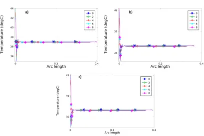
Figure 4.1. Spherical head model – SHM_04 a) BF, b) BL and c) RUL configurations showing the temperature distribution at 8 s. ... 46 Figure 4.2. Graphic of temperature (ºC) along the time (s) for the point of maximum temperature, for 800 mA. a) BF, b) BL and c) RUL. ... 47 Figure 4.3. Wireframe of the spherical head model showing the position of the line used to analyse the temperature in the configurations a) BF, b) BL and c) RUL. The first point of this line represents the maximum temperature... 47 Figure 4.4. Graphic of Temperature (ºC) along the arc length (Figure 4.3) showing the distribution of temperature in 5 different times 0 s, 2 s, 4 s, 6 s and 8 s. a) BF, b) BL and c) RUL. ... 48
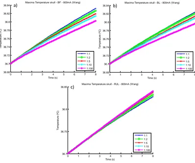
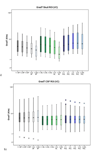
Figure 5.1. Spherical head model with five layers, for different electrode montages (a) BF, (b) BL and (c) RUL. The region marked in blue specifies the ROI. ... 53 Figure 5.2. Plot of the point of maximum temperature in the skull, over time, for isotropic and anisotropic (Wang) cases, for the three electrode configurations (a) BF, (b) BL and (c) RUL. Shown here for 800 mA. ... 56 Figure 5.3. Percentage difference from Tmax at t = 8 s comparing with T0 (a); and
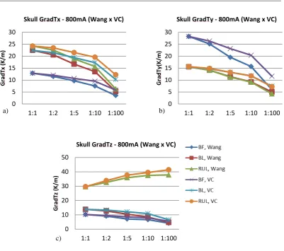
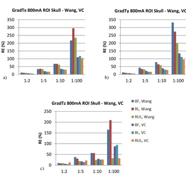
GradTz, at ROI skull. BF (grey), BL (green) and RUL (blue); isotropic to anisotropic goes from darker to lighter colour tone. VC 800 mA input at t = 8 s. ... 61 Figure 5.7. Graphic showing the behaviour of GradT directional maximum (K/m) in function of anisotropic ratio. Comparison between Wang and VC is made. Input of 800 mA at t = 8 s. (a) GradTx, (b) GradTy and (c) GradTz. ... 62 Figure 5.8. Comparison of the isotropic and anisotropic model simulations in the ROI for BF (VC, 800 mA input). The false color map shows Tmax (ºC) behaviour, the
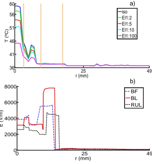
contour plot shows the GradT (K/m) and the white arrows the E-field for the cases (a) 1:1 (isotropic); and anisotropic for rations (b) 1:2, (c) 1:5, (d) 1:10 and (e) 1:100. ... 63 Figure 5.9. Relative error of gradient of temperature magnitude for the entire ROI (a) and each layer of the model (b) scalp, (c) skull, (d) CSF, (e) GM and (f) WM for each electrode configuration and all the anisotropic ratios (1:2, 1:5, 1:10, 1:100). Shown here for Wang constraint, 800 mA. ... 64 Figure 5.10. Comparison between relative error of maximum gradient of temperature from skull, for Wang and Volume constraint, 800mA input, t = 8 s. (a) GradTx; (b)
GradTy; and (c) GradTz. ... 65
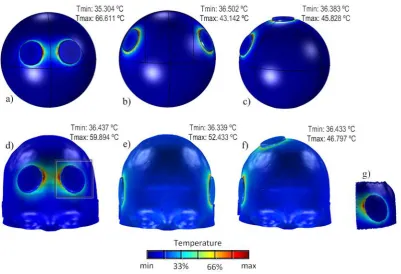
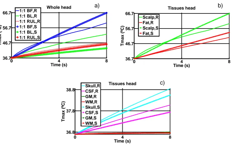
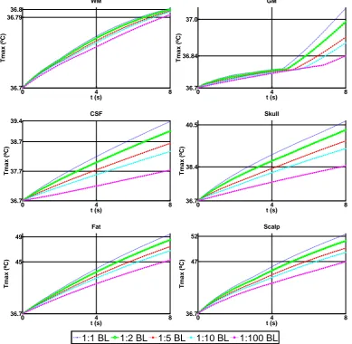
Figure 6.1. Models showing the electrode montage (a) BF, (b) BL and (c) RUL SHM; and (d) BF, (e) BL and (f) RUL RHM. The black box in image (d) represents the (g) ROI. The colour map represents temperature. ... 71 Figure 6.2. Tmax (ºC) as a function of time for realistic (R) and spherical (S) models,
among CSF, GM and WM are not shown; and b) E-field, isotropic, BF, BL, RUL. 78 Figure 6.4. E-field distribution in a non-homogeneous medium along axial plane for BF-RHM. The magenta arrows represent current density. a) isotropic and b) El1:10. ... 78 Figure 6.5. Comparison of Tmax for four different setups (RHM), BL electrode
configuration. isotropic (1:1) versus 4 anisotropy ratios (1:2, 1:5, 1:10, 1:100), when considering thermal and electrical conductivity in the skull layer. ... 81 Figure 6.6. Comparison of Tmax for isotropic versus anisotropic, BL montage –
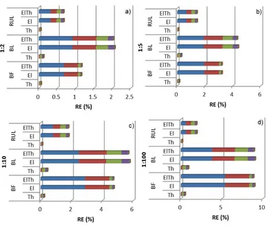
thermal (Th), electrical (El) and thermal-electrical (ElTh), at ratio 1:10, in the skull layer. ... 82 Figure 6.7. Temperature RE (%) of anisotropic (a) 1:2, (b) 1:5, (c) 1:10 and (d) 1:100 models from ROI; thermal (Th), electrical (El) and thermal+electrical (ElTh), for BF, BL and RUL on RHM. Each colour relates to one head tissue, scalp (dark blue), fat (red), skull (green), CSF (purple), GM (light blue) and WM (orange). ... 83 Figure 6.8. Behaviour of Tmax (ºC), in each tissue layer, for different current (A)
Figure 7.1. 3D brain geometry showing slices of a 30º plane (a) crossing both tumors, delineated magenta area for tumor RFL and grey area for tumor LOL. Slices of brain tumor, with the false color map being the magnitude of E-field and current density represented by the black arrows. (b, c) BF; (d, e) BL and (f, g) RUL. ISO – isotropic; ANISO – anisotropic. ... 100 Figure 7.2. Maximum E-field magnitude for the isotropic and anisotropic control cases, at different ROIs (a) GM, (b) WM, (c) hippocampus, (d) thalamus, (e) tumor RFL, (f) tumor LOL and (g) ventricles. ... 102 Figure 7.3. Median E-field magnitude for the isotropic and anisotropic control cases, at different ROIs (a) GM, (b) WM, (c) hippocampus, (d) thalamus, (e) tumor RFL, (f) tumor LOL and (g) ventricles. ... 103 Figure 7.4. RE E-field magnitude at control case for different ROIs (a) GM, (b) WM, (c) hippocampus, (d) thalamus, (e) tumor RFL, (f) tumor LOL and (g) ventricles. 104 Figure 7.5. Percentage of the total volume that exceeds the E-field in the horizontal axis (V/cm), for three electrode configurations, control isotropic and anisotropic cases and different ROIs (a) GM, (b) WM, (c) hippocampus, (d) thalamus, (e) tumor RFL, (f) tumor LOL and (g) ventricles. ... 106 Figure 7.6. Graph of Emed for the control case and the four different tumor grades
(tumor 1) at second column, for all tumor grades, at BF (first row), BL (second row) and RUL (third row)... 112
List of Tables
Table 3.1. Summary of the human head models. ... 42
Table 4.1. Electrical and thermophysical properties of head tissues. ... 44
Table 5.1. Simulated values for the skull thermal conductivity tensor eigenvalues for the VC and Wang. Units of k in W/m.K. ... 54
Table 6.1. Thermophysical and electrical properties of fat. ... 72 Table 6.2. Values used to simulate the skull. Units of k and σ in W/m.K and S/m, respectively. ... 74 Table 6.3. Thermophysical and electrical properties of the scalp for interface electrode-skin study. ... 75 Table 6.4. Tmax, at t=8s, in each tissue layer for isotropic case, RHM and SHM. ... 76
Table 6.5. Tmax in the skull layer for isotropic (iso) and skull anisotropic conductivity
ECT stimulation for BF, BL and RUL electrode configuration... 88
Table 7.1. Isotropic electrical conductivity of tissues (Datta, Elwassif & Bikson 2009; Hasgall PA 2014). ... 99
“If you realized how powerful your thoughts are, you would never think
a negative thought.”
1. INTRODUCTION
1.1.
Background
The human brain is the most interesting and unknown organ in the human body. It lies in the cranium, being protected by the skull. The brain gives commands to and receives requests from the entire body through connections among the trunk and limbs through the spinal cord (Standring 2015). It can mainly be divided into frontal, temporal, parietal, occipital and insula.
The human brain is always incognito and it is common to find people with some kind of neurological issues, where frequently, the problem is unknown and the treatment is difficult. Pharmacotherapy is normally used to treat brain diseases, but this is not always effective and, can sometimes cause other problems. Another type of treatment which has been used for decades is transcranial electrical stimulation (tES), where a stimulus is delivered to the scalp or inside the head, directly to the brain. As in all kinds of treatment, side effects can also happen, but studies and practices have demonstrated good, promising and efficient results in many cases.
2013) is known as electroconvulsive therapy (ECT). There are many polemics in the use of this technique, because whereas some people say that this technique can treat and help extreme cases of neurological diseases, others say that this technique is too aggressive, with significant side effects and its use should be ceased. With the pur-pose of trying to demystify, better understand and make it safer, the focus of this study is on this therapy.
All these techniques use electrical current input and, in the case of electroconvulsive therapy high current is used, so particular care should be taken. As we know, when electrical current passes through a conductor, heat is generated. Temperature (T) in-creases due to Joule heating and metabolic responses which are a result of electrical stimulation of tissues (Datta, Elwassif & Bikson 2009; Elwassif et al. 2006). Electri-cal stimulation-induced changes in temperature can profoundly affect tissue function (Elwassif et al. 2006). Moreover, metabolic response occurs in the human head as a result of electrical stimulation. This heat is distributed over body regions by blood circulation and is carried by conduction to the body surface (Fiala, Lomas & Stohrer 1999). Both effects, Joule heat and metabolic response, are causes of temperature increase (Datta, Elwassif & Bikson 2009; Elwassif et al. 2006). How the heat affects the different tissue layers of the head while electroconvulsive therapy is applied has not yet been investigated thoroughly.
issues. However, a realistic head model, with its true anatomical features and con-ductivity behaviour, help us to study these cases and achieve comprehensive results. Having all these limitations in mind, this study aims to investigate the distribution of temperature and temperature gradient due to high electrical stimulation used in ECT treatments. Beyond that, the models also consider the inhomogeneous and aniso-tropic thermal and electrical conductivity along the tissues. Magnetic resonance im-aging (MRI) and diffusion tensor image (DTI) data are used and, with this, the issues of structural head model details and directional conductivity are addressed respec-tively. Finite element methods (FEM) possess the ability to consider complex ge-ometries and anisotropic behaviour without discretization errors. Taking this into ac-count, the commercially available FE package COMSOL Multiphysics ® is used to generate and map the thermal and electric field distributions.
With this study, a better understanding of the effects induced by high-stimulation in the thermal point of view is achieved; also, potential damage to any structure of the human head and how this heat influences the neurons and regions of the head is ex-amined. Moreover, it also provides a better understanding of electric field distribu-tion in the human head, in the presence of a brain tumor. The study is implemented using computational simulation and no live or deceased biological samples are used. To validate the results, mathematical models, bio-heat transfer equation (BHTE) linked with Laplace equation applied to electrics and resistive-capacitive network are used.
1.2.
Aim and Objectives
real-geted:
1. Realistic human head construction and modelling from thermal and electrical conductive aspects.
2. Investigation of the temperature behaviour in a spherical and realistic human head model under isotropic and anisotropic conductivity conditions.
3. Analysis of the combined effect of temperature and the electrical activities in a human head model.
4. Analysis of the influence of thermophysical parameters and fat layer on the temperature behaviour.
5. The usage of ECT on patients with a brain tumor.
1.3.
Research Strategy
This study investigates the influence of thermal and electric fields due to electrical stimulation when electroconvulsive therapy is applied. Spherical and realistic head models will be developed using commercial packages. Different configurations using heterogeneous tissues, isotropic and thermal and electrical anisotropic conductivity and diverse electrode montage, will be considered. At first, a simplified spherical head model is built, as it is easier to construct and understand. From there onwards, a more sophisticated, realistic head model will be developed and constructed using magnetic resonance images. An assumption of linearity between thermal and electri-cal conductivity was made based on the fact that there is a linearity relationship be-tween their eigenvalues. This assumption will be used to derive the thermal anisotro-py on the skull, with thermal and electrical anisotroanisotro-py conductivity being mathemati-cally applied. Later on, diffusion tensor images will be inserted in the realistic mod-els to consider white matter electrical anisotropy. Also, the presence and influence of a brain tumor will also be considered.
computation-1.4.
Thesis Overview
This dissertation consists of eight chapters. The first three chapters provide the re-search background, a comprehensive literature review about the rere-search and the methodology applied. Chapters 4 to 7 illustrate the diverse cases of the models’ de-sign, development, implementation and outcomes in assessing the induced thermal and electric field and their parameters.
Chapter 2 presents an overview of the current transcranial electrical stimulation techniques and their applications. It focuses on electroconvulsive therapy, its usages, properties and parameters, and provides a detailed explanation about bio-thermal models and the sensitivity of the human body to the temperature.
Subsequently, the chapter provides the mathematical background that will be applied in the model developments. Among these formulae are the Maxwell’s equation, its simplified quasi-static approximation, the bio-heat transfer equation, the initial and boundary conditions required to define a problem. It also describes the assignment of thermal and electrical conductivity to each of different head tissues.
Chapter 3 describes the techniques and methods to develop the three head models used in this study. It starts with the spherical model and ends with a realistic one. The chapter provides step by step explanations of techniques and methods used in the model development. In addition, the electrode montages are also considered and ex-plained.
Chapter 4 analyses the behaviour of temperature due to ECT electrical stimulation using a simplified four layer spherical model. The bio-heat transfer equation and the Laplace equation are coupled together to solve the problem. Three different electrode montages are considered with two different amplitude inputs. The models are studied using FEM.
con-pared with the isotropic ones.
Chapter 6 extends the method used in Chapter 5 considering more layers in a realis-tic head model. In addition, the influence of including anisotropy electrical conduc-tivity in the skull layer is investigated. Apart from that, the role and effect of biologi-cal properties and the influence of fat layer in the thermal behaviour are also ex-plored.
Chapter 7 describes the electric field distribution when ECT stimulation is applied to a patient with a brain tumor. Four diverse tumor grades, varying according to tu-mor aggressiveness, are conducted; as well as two different tutu-mor locations and three electrode configurations. In addition, white matter anisotropy is assigned from diffu-sion tensor images and the models with anisotropy are compared with isotropic ones as reference models.
2. ELECTROCONVULSIVE THERAPY AND
BIO-THERMAL MODELS
2.1.
TES and Human Head Model
Transcranial Electrical Stimulation encompasses all forms of research and clinical application of electrical currents to the brain using (at least one) electrodes on the head (Cancelli et al. 2016; Casarotto et al. 2013; Chen et al. 2017; Datta, Elwassif & Bikson 2009; Elwassif et al. 2012; Elwassif et al. 2006; Fertonani & Miniussi 2016; Guleyupoglu et al. 2013; Lee et al. 2012; Peterchev et al. 2012; Wagner, Valero-Cabre & Pascual-Leone 2007). Although not always popular, techniques of transcra-nial electrical stimulation date back further than one century. At the beginning, it was applied to treat neurological diseases and through time, new methods were invented and the existing ones modified to achieve more accurate results. TES is an alternative to pharmacological treatment in neurological diseases. It can enhance cognitive per-formance in healthy people and improve clinical conditions in patients (Fertonani & Miniussi 2016).
transcranial Sinusoidal Direct Current Stimulation (tSDCS), and transcranial Ran-dom Noise Stimulation (tRNS)).
All these techniques aim to study the behaviour of the brain and provide valuable tools to treat a variety of neurological and psychiatric disorders (Wagner, Valero-Cabre & Pascual-Leone 2007).
One of the inherent problems with these treatments is the need to always consider the correct dosage to be used, as well as the side effects they can cause. Dosage depends on electrode montage and stimulation waveform that is applied trough the electrodes (Guleyupoglu et al. 2013; Peterchev et al. 2010; Peterchev et al. 2012). The electrode parameters include number, position, shape, and composition. Stimulation waveform considers details such as intensity, pulse shape, amplitude, width, polarity, and repe-tition frequency, duration of and interval between bursts or trains of pulses, and in-terval between stimulation sessions and total number of sessions (Guleyupoglu et al. 2013).
A human head model is used to simulate different cases of tES problem. These mod-els help investigate and develop those techniques. At first, analytical solutions were developed to calculate spherical homogeneous volume conductors, as seen in Frank (1952). Then, inhomogeneous volume conductors started to be studied like in Salu et al. (1990) and in Rush and Driscoll (1969). The former represented the head as a three-layer spherical model and evaluated the localization of equivalent dipoles in the brain, and the latter proposed a 3-layer spherical volume conductor consisting of scalp, skull and brain, and gave a better understanding of the behaviour of current density distribution inside an inhomogeneous head model. Therefore, De Munck (1988) incorporated a semi-analytical solution to deal with anisotropy in a layered spherical and spheroidal volume conductor; and Zhou and van Oosterom (1992) ap-plied a semi-analytical procedure considering four layer isotropic and anisotropic concentric spherical volume conductor.
through different tissue layers. MRI also permits us to verify more appropriate sites to localize electrodes, dosage and duration of the stimulation, among other factors. An example is shown in the work of Bai, Loo and Dokos (2011), in which they mod-elled a realistic head model to compare the effects of electric field spatial profiles and brain excitation when three different ECT electrode configurations were used. A detailed high-resolution realistic human and neck head model, including 153 struc-tures, arteries and veins from magnetic resonance angiography (MRA) and diffusion tensor information was developed by Iacono et al. (2015). They applied tACS to il-lustrate the application. The MIDA model, as it is now called, still provides more de-tails and structural variation than any other model so far developed.
The inclusion of DT-MRI data permitted even more accurate analyses. With more refined geometries of the human head available, it became possible to analyse more factors, such as brain structures and anisotropic conductivity for different tissues. Oostendorp et al. (2008) proposed a method to estimate the potential and current density distribution during tDCS in a five compartment realistic head model. In their study, they included anisotropic electrical conductivity to the skull and white matter. In the study of Datta et al. (2009), they applied a high spatial resolution MRI derived finite element human head model and resolved cortical gyri/sulci. They compared the spatial focality of conventional rectangular pad (7 x 5 cm2) and ring (4 x 1) electrode configurations. They suggested that anatomically accurate high resolution MRI based forward models may guide the rational clinical design and optimization for tES tech-niques. Many other studies can be found which use high resolution human head model (Bai, Loo & Dokos 2011; Datta, Elwassif & Bikson 2009; Lee et al. 2012; Lee et al. 2011; Shahid, Wen & Ahfock 2013).
2.2.
Electroconvulsive Therapy
Schizophrenia, Bipolar manic (and mixed) states, Catatonia and Schizoaffective dis-order (Weiner 2002). This therapeutic intervention applies an electric voltage or cur-rent to the scalp through electrodes (Lee et al. 2012). The induced electric field is typically widespread and reaches deep brain regions (Rosa & Lisanby 2012). The patient should receive a muscle relaxant and general anesthesia before the procedure. The stimulation is generated in cycles that vary from 0.5 to 8 seconds of duration, the frequency varies between 20 Hz and 120 Hz, and the pulse currents vary from 500 mA to 900 mA (Weiner 2002). The entire procedure can be completed in approxi-mately 10 minutes.
Figure 2.1. Illustration showing electroconvulsive therapy treatment (NIMH 2016).
important to maximize efficacy and tolerability (Lee et al. 2012; Weiner 2002). These factors can affect the clinical outcome (Weiner 2002).
The physical properties of ECT stimulus affect efficacy and cognitive side effects (Sackeim et al. 1994). Some of the side effects include problems of general anaesthe-sia, memory loss, possibility of aggravating problems inside the head, possibility of getting uncontrollable fits or status epilepticus (Weiner 2002). Although improve-ments have been made in ECT throughout time, many questions still need to be an-swered (Lee et al. 2012). For example, what is the best electrode configuration for the practice of ECT? How do we reduce and avoid side effects? Which are the best stimulus current parameters for maximal efficacy and tolerability? What is the influ-ence of heat transfer in this procedure? etc.
Ultrabrief pulse has been recently used to further improve the risk–benefit ratio of ECT (Loo et al. 2012). This approach substantially reduces the cognitive side effects without loss of efficacy, although a response may take longer and mid-course dose adjustments may be necessary to ensure efficacy (Rosa & Lisanby 2012).
A study conducted by Swartz (1989) dealing with heat liberation at the electrode-skin interface during ECT stimulus, reported that the electrode-skin was the only possible site for an electrical burn with ECT devices from his time. The explanation he gave was that the substantial deep tissue heating (as in the brain) does not occur, because the typical maximum output of an ECT device (100 J at 220 Ω impedance) elevates deep tissue temperature by less than 0.092 ºC. He concluded that if there was a poor elec-trode-skin contact, then skin burn could occur.
Lee et al. (2012) investigated the electric field (E-field) strength generated by various ECT electrode configurations in specific brain regions of interest (ROIs) that have putative roles in the therapeutic action and/or adverse side effects of ECT. They also characterized the impact of the white matter conductivity anisotropy on the E-field distribution. A finite element head model incorporating tissue heterogeneity and WM anisotropic electrical conductivity based on structural MRI and DT-MRI data was constructed. The spatial E-field distributions were computed with the ECT electrode placements BL, BF, RUL and FEAST. The results show that the median E-field strength over the whole brain is 3.9, 1.5, 2.3, and 2.6 V/cm for the BL, BF, RUL, and FEAST electrode configurations respectively. They also found that neglecting the WM electrical conductivity anisotropy produces E-field strength error up to 18% overall and up to 39% in specific ROIs, motivating the inclusion of the white matter electrical conductivity anisotropy in accurate head models.
When comparing ECT with TMS (transcranial magnetic stimulation) in depression treatment, it has been found that ECT is the most efficacious, but it is difficult for patients to tolerate. The review done by Chen et al. (2017), the efficiency of ECT is 65 %, and, according to the TMS setup used, the efficiency varies from 2 to 25 %. On the other hand, ECT tolerability is only 14 %, while TMS is 16 % to 52 %. How-ever, ECT generates from 3 to 29 times more stimulation in areas related to antide-pressant effect, such as thalamus, hypothalamus and hippocampus (Lee et al. 2016).
2.3.
Bio-thermal Model
network function (Datta, Elwassif & Bikson 2009; Elwassif et al. 2006). Tempera-tures above 40 ºC in the human body can result in cell damage and tissue ablation (Elwassif et al. 2006). Metabolic processes in the organism try to compensate for this excessive heating in an attempt to preserve the temperature at an acceptable level (Zaridze et al. 2005).
Two areas in which brain and body temperature may have a crucial impact are neu-rodegenerative and mood disorders. Many failures in temperature control have been observed in psychiatric conditions. Salerian, Saleri and Salerian (2008) have pro-posed a temperature-dependent biochemical system in humans governed by the Ar-rhenius rate law. They postulated that due to the exponential relationship between temperature and biochemical reactions, a relatively minor alteration in core body or brain temperature may be of significant therapeutic benefit in combating neuro-degenerative disorders and prolonging lifetime. They speculated that this small alter-ation may be as little as a drop of 1 ºC in core body temperature.
Investigations on the effect of electroconvulsive shock (ECS) on body temperature have been contradictory. A single ECS has been demonstrated to reduce colonic temperature in mice. However, repeated ECS attenuates the hypothermia produced by single ECS. Application of single ECT is hypothermic and it improves mania. Chronic ECT is thermogenic and it improves depression (Salerian, Saleri & Salerian 2008).
stimula-A healthy human brain was modelled thermally as a 3-concentric spherical model using finite element method by Lillicrap et al. (2012) to investigate the effectiveness of tissue cooling as a result of spatial variations in cerebral blood flow and cerebral metabolic rate. These factors were found to affect the absolute level of tissue cooling achievable, but not the rate of cooling.
A Eulerian approach for the numerical solution of the transient bio-heat transfer equation with temperature-dependent properties was developed by Bourantas et al. (2014). They extended the bio-heat equation in order to incorporate water evapora-tion and tissue damage during ablaevapora-tion, accounting for temperature-dependent ther-mal properties of the tissue. This approach treated 3D heat conduction problems within pathological tissues of locally varying conductivity and locally varying blood perfusion rate, viewing them as continuous domains, and solving the corresponding bio-heat differential equation with variable coefficients. In addition, they showed that arbitrary and random conductivity maps can be treated in a straightforward manner with this method in contrast to the flux continuity technique that is not applicable in the case of vaguely defined boundaries.
Datta, Elwassif and Bikson (2009) provided information on the thermal effects of tDCS using a MRI-derived finite element human head model. A bio-heat model (coupled Laplace equation of an electric field and the Pennes bio-heat transfer equa-tion) were solved to compare the tissue temperature increases of tDCS using conven-tional rectangular-pad (7 x 5 cm2) and HD-tDCS using the ring (4 x 1) electrode con-figurations. The results indicated that clinical tDCS do not increase tissue tempera-ture and 4 x 1 ring configurations leads to a negligible increase in scalp temperatempera-ture. However, the study did not consider micro architecture of the skin, nor variation in the electrical and thermal properties. A clinical tDCS study (Ezquerro et al. 2016) evaluated the skin redness over a crossover trial. They found mild to moderate ery-thema after tDCS-induced stimulation.
Another study of the thermal effects of DBS was conducted by Elwassif et al. (2012). They developed a heat transfer finite element method simulating DBS incorporating the realistic architecture of Medtronic 3389 leads. The temperature changes were an-alysed considering different electrode configurations, stimulation protocols and tis-sue properties. The results were then validated using micro-thermocouple measure-ments during DBS lead stimulation in a saline bath. FEM results indicated that lead design (materials and geometry) may have a central role in controlling temperature rise by conducting heat. Apart from that, a temperature increase was found to depend on root mean squared voltages rather than waveform details, and the electrode volt-age attenuation was assumed to be inherently reversible capacitive (or reversal fara-daic) and thus with no power dissipation (this reversibility is indeed expected for a chronically implanted device). They showed how modifying lead design could effec-tively control temperature increases. Also in the DBS field, Iacono et al. (2013) modelled a millimetric resolution and multiscale head model to analyse the accuracy of numerical modelling of a radio-frequency field when a patient has a DBS elec-trode implanted. However, they computed only an electric field and local SAR, and a thermal evaluation was not considered.
10 and 900 MHz) inside a detailed anatomical heterogeneous human body model us-ing the finite-difference time-domain method. The correspondus-ing temperature in-crease was evaluated through an explicit finite-difference formulation of the bio-heat equation. The thermal model was composed by a controlling and controlled system, which took into account the thermoregulatory system of the human body, and was validated through a comparison with experimental data. This study aimed to investi-gate the relation between limits settled in the safety standards and the thresholds for the induction of adverse thermal effects. While Nadobny et al. (2007), performed an investigation of magnetic resonance (MR)-induced hot spots in a high-resolution human model. The study analysed the temporal SAR mode (steady imaging and in-termittent imaging); the simulation procedure (related to given power levels or to limiting temperatures); and different thermal tissue properties including temperature-independent and temperature-dependent perfusion models. The electromagnetic and thermodynamic studies were carried out in simulations.
Studies considering anisotropic thermal conductivity are found in the study of both human and animal eyes. Berjano, Saiz and Ferrero (2002) presented a theoretical model for the study of cornea heating with radio-frequency currents. Their numerical model allowed the study of the temperature distributions in the cornea, by solving a coupled electric-thermal problem, and to estimate the dimensions of the lesion in the cornea. They analysed the effect of temperature influence on the tissue electrical conductivity; the dispersion of the biological characteristics; the anisotropy of the cornea thermal conductivity; the presence of the tear film; and the insertion depth of the active electrode in the cornea. Their results suggested that these effects have a significant influence on the temperature distributions and thereby on the lesion di-mensions. Both their study and the work of Trembly and Keates (1991) suggested that conductivity is larger in the longitudinal direction (parallel to the corneal sur-face) than transverse direction. The study done by Berjano, Saiz and Ferrero (2002) involved temperature profile geometry with a more ellipsoidal shape (width/depth ratio of 1.3) and they concluded that there is a direct relation between maximum temperature (Tmax) and the temperature profile dimensions. In the study of
component of thermal conductivity larger than the transverse one led to a smoother temperature variation along the vertical axis of the corneal surface. Also in the study of Barton and Trembly (2013) they stated that the anisotropy of the thermal conduc-tivity of the cornea might be known, in order to quantify the balance of heat transfer toward the epithelial and endothelial layers and parallel to them.
2.4.
Quasi-static Approximation and Bio-heat
Trans-fer Equation
When the frequency is low, from direct current (DC) to 10 kHz, biological material exhibits strong resistivity behaviour. Therefore, Maxwell’s equation can be simpli-fied to the quasi-static approximation (Bai, Loo & Dokos 2013; Ferdjallah, Bostick & Barr 1996; Malmivuo & Plonsey 1995; Shahid 2013). According to Ohm’s law and supposing electric field strength, E, throughout a passive volume conductor model, has the Laplace partial differential equation:
𝜵 ∙(−𝝈𝜵𝝈) =𝟎 or 𝜵 ∙ �
𝝈𝒙𝒙 𝝈𝒙𝒙 𝝈𝒙𝒙
𝝈𝒙𝒙 𝝈𝒙𝒙 𝝈𝒙𝒙
𝝈𝒙𝒙 𝝈𝒙𝒙 𝝈𝒙𝒙
� �𝝏𝝈 𝝏𝒙𝝏𝝈 𝝏𝒙⁄⁄ 𝝏𝝈 𝝏𝒙⁄ �= 𝟎
in Ω ( 1 )
Equation 1
where σ and V are the electrical conductivity and the scalar electric potential in a volume Ω.
𝝆𝝆𝝏𝝏𝝏𝝏 = 𝛁(𝒌𝛁𝝏) +𝝎𝝆𝒃𝝆𝒃(𝝏𝒂− 𝝏) +𝑸𝒎 ( 2 ) Equation 2
where ρ: density (kg/m3), c: heat capacity (J/(kg.ºC)), k: thermal conductivity (W/(m.ºC)), T: temperature (ºC), Ta: arterial blood temperature (ºC), ωb: blood perfu-sion rate (1/s), Qmet: metabolic heat source (W/m3), and the subscript b denotes blood (Bezerra, L. et al. 2013; Datta, Elwassif & Bikson 2009; Silay, Dehollain & Declercq 2008). The term from the left hand side is related to the rate of stored energy in the tissue mass that balances the equation. The first term from the right hand side is re-lated to the rate of input and output energy; the second term is an additional amount related to heat transfer from blood flow, that is, the energy added or removed due to the convective blood flow into and out of the tissue; and the last term is the genera-tion of metabolic heat (Berger, Goldsmith & Lewis 1996; Christian, Firebaugh & Smith 2012).
The thermal conductivity is also a scalar number in the case of isotropic volume con-ductors. For anisotropic conductors, k is a tensor (Equation 3), where it is possible to consider its preferential directions of current flow (Lewis et al. 1996).
𝒌= �
𝒌𝒙𝒙 𝒌𝒙𝒙 𝒌𝒙𝒙
𝒌𝒙𝒙 𝒌𝒙𝒙 𝒌𝒙𝒙
𝒌𝒙𝒙 𝒌𝒙𝒙 𝒌𝒙𝒙
� ( 3 )
Equation 3
In transcranial electrical stimulation, current is applied through the electrodes. The electrical stimulation generates heat which increases the temperature and the temper-ature variation can also occur along the tissue of the head. Taking this into considera-tion, the physics applied involves heat transfer and electrical potential simultaneously (Datta, Elwassif & Bikson 2009; Elwassif et al. 2012; Elwassif et al. 2006):
2.4.1. Initial and Boundary Conditions
Both Maxwell’s and bio-heat transfer equations need specifications of the required initial (IC) and boundary conditions (BC) (Figure 2.2) to completely formulate the problem. For the electrical physics, the exposed boundaries (Γe) are considered elec-trically insulated and are represented by Neumann boundary conditions:
𝒏 ∙ 𝑱|𝜞𝒆 =𝟎 or 𝒏 ∙(𝝈𝜵𝝈)|𝜞𝒆=0. ( 5 ) Equation 5
The inner boundaries (Γi) are expressed by the continuity of the normal component of the current density between regions of different conductivity:
(𝒏 ∙ 𝑱𝟏)|𝜞𝒊 = (𝒏 ∙ 𝑱𝟐)|𝜞𝒊 or [𝒏 ∙(𝝈𝜵𝝈𝟏)]|𝜞𝒊 = [𝒏 ∙(𝝈𝜵𝝈𝟐)]|𝜞𝒊 ( 6 ) Equation 6
The exposed surface of the cathode (Γs) is assigned the Dirichlet boundary (V=0
volts) condition, whereas, the exposed surface of the anode (Γs) can be assigned with either the Dirichlet (V=V0 volts) or the Neumann (n·J = Jn A/m2) BC, where V0 is the fixed electrode voltage and Jn is the surface current density normal to the electrode surface.
k1
k2
k3
Figure 2.2. Model showing thermal and electrical BC.
For the thermal physics, convection occurs in the external surface of the head model
(Γe), and thus, heat flux is assigned to the external BC:
−𝒌 ∙𝝏𝝏𝝏𝒏= 𝒉 ∙(𝝏𝒂𝒎𝒃− 𝝏). ( 7 ) Equation 7
where h is the heat transfer coefficient and Tamb is the external temperature.
This equation is also known as Newton law of cooling. In the interfaces of the head conduction occurs between two layers and equation 8 can be assigned:
𝒌𝟏𝝏𝝏𝝏𝒙𝟏�𝜞 𝒊 =𝒌𝟐
𝝏𝝏𝟐
𝝏𝒙�𝜞𝒊 ( 8 )
Equation 8
2.5.
Electrical and Thermal Conductivity
Represen-tations
2.5.1. Anisotropic Electrical Conductivity
Some regions of the head present anisotropic electrical conductivity (De Munck 1988; Marin et al. 1998; van den Broek et al. 1998; Wolters et al. 2006). The expres-sion that gives the anisotropic electrical conductivity is found in the literature and is usually given in local coordinates as:
𝝈𝒔𝒌𝒔𝒔𝒔=�
𝝈𝝏 𝟎 𝟎
𝟎 𝝈𝝏 𝟎
𝟎 𝟎 𝝈𝑹
� ( 9 )
Equation 9
where 𝜎𝑆𝑆𝑆𝑆𝑆 is a second rank symmetric tensor ( )
T
SKULL SKULL
There are certain methods and approaches to calculate the electrical conductivity from the diffusion weighted MRI. One is a linear relationship that relates the eigen-values and the tensor (Haueisen et al. 2002):
𝝈 =𝝈𝒆
𝒅𝒆𝑫 ( 10 ) Equation 10
where 𝜎𝑒 and 𝑑𝑒 are the effective extracellular conductivity and diffusivity, respec-tively; D is the diffusion tensor; and the intracellular conductivity is assumed to be negligible. Another approach is the volume constraint (VC) (Wolters et al. 2006) which considers that eigenvalues must retain their geometric mean, and thus, the volume of the conductivity tensor:
𝟒
𝟑𝝅𝝈𝑹(𝝈𝝏)𝟐 = 𝟒
𝟑𝝅𝝈𝒊𝒔𝒊𝟑 . ( 11 )
Equation 11
A third approach is obtained combining equations (10) and (11) and using a matrix to represent the diffusion tensor in a voxel belonging to the WM (Hallez et al. 2008):
𝒅𝟏 𝝈𝟏 =
𝒅𝟐 𝝈𝟐 =
𝒅𝟑
𝝈𝟑 ( 12 ) Equation 12
Another method is the Wang constraint (Wang) (Wang, Haynor & Kim 2001), where the product of radial and tangential conductivity should remain constant and be equal to the square of the isotropic conductivity:
𝝈𝑹𝝈𝝏= 𝝈𝒔𝒌𝒔𝒔𝒔𝟐 . ( 13 ) Equation 13
2.5.2. Anisotropic Thermal Conductivity
In this approach, the BHTE is discretized by applying a forward-intime, central-in-space (FTCS) explicit FD scheme, as follows:
𝝏𝝉+𝟏 ≅ 𝝏𝝉∙𝑪+𝑫𝝉+𝑩𝝉
𝑨𝝉 ( 14 ) Equation 14
where 𝐴𝜏 =𝜔𝜏𝜌𝑏𝑐𝑏+𝜌𝑐 ∆𝑡⁄ , 𝐵𝜏 =𝜔𝜏𝜌𝑏𝑐𝑏𝑇𝑏 and 𝐶= 𝜌𝑐 ∆𝑡⁄ . τ is the consecutive number of the time step with the length ∆t. Dτ is the discretized conductive term for 𝑑𝑑𝑑(𝜅𝜅𝜅𝜅𝑑𝑇) which is dependent on the temperature gradients Gx, Gy and Gz. The conductivities 𝜅𝑥/𝑦/𝑧 are calculated via series connections of the original (nonaver-aged) conductivity values κ in neighbouring cubes. Therefore, they are direction de-pendent being numerically induced anisotropy near the thermal interfaces.
To avoid staircase errors, the exterior boundaries need to be written in vector formu-lation (Nadobny et al. 2007):
𝒒��⃗ ≅ −𝜿𝝏𝝏𝝏𝒏𝒏��⃗𝑶 = −𝜿 ∙ 𝑮��⃗
𝒏 ≅ 𝒉 ∙(𝝏 − 𝝏𝒆𝒙𝝏)∙ 𝒏��⃗𝑶 ( 15 ) Equation 15
where 𝑞⃗ is the conduction heat flux vector, 𝑛�⃗𝑂 is the unit surface normal vector, and
𝐺⃗𝑛 is the normal temperature gradient vector.
2.5.3. The Relation between Thermal and Electrical
Conduc-tivity
A linearity between thermal conductivity tensor and electrical conductivity tensor is found in the literature (Khundrakpam, Shukla & Roy 2010). The model for the rela-tionship between electrical and thermal conductivity (Figure 2.3) is based on the ef-fective medium approach for two-phase anisotropic media. The relationship of the effective transport tensor to the microstructure is written as:
�𝜶𝒆𝒆𝒆� 𝜶𝒆 = �𝑹
(𝒊)�[𝑷
where 𝛼 denotes either thermal or electrical conductivity; the subscripts eff and e de-note tensors to the microstructure and transport coefficients in the host phase (basic interstitial matrix), respectively; �𝑅(𝑖)� is a concatenated series containing micro-structure information; and, [𝑃𝛼] is a concatenated series of 𝛼. Therefore, it is possible to obtain a cross-property relationship between the two transport tensors:
𝜿𝒗= 𝒂𝟏(𝝈𝒗±𝝆𝟏) ( 17 ) Equation 17
where 𝜅𝑣 and 𝜎𝑣 are the eigenvalues of the thermal conductivity tensor and electrical conductivity tensor, respectively, while 𝜅1 and 𝑐1 are numerical constants.
Figure 2.3. Experimental validation of cross-property relationship between thermal conduc-tivity and electrical conducconduc-tivity values of various tissues. Electrical and thermal
conductivi-ty eigenvalues (data points from left to right: white matter, grey matter, cerebral cortex,
cer-ebellum, spleen, liver, kidney and heart) (Khundrakpam, Shukla & Roy 2010).
tissue on the electrical conductivity will be verified. This procedure and verification has never been used previously in ECT analysis.
2.6.
Discussions of Reviewed Works
ECT has been detailed studied under the electrical perspective, as can be found in the literature (Bai 2012; Bai et al. 2012; Bai, Loo & Dokos 2011; Casarotto et al. 2013; Lee et al. 2016; Lee et al. 2012; Lee et al. 2011; Loo et al. 2012; Peterchev et al. 2010; Rosa & Lisanby 2012; Sackeim et al. 1994; Swartz 1989; Weiner 2002). From the simplistic models to more realistic geometries, the consideration of isotropic tis-sues and electrical anisotropy tistis-sues, diverse electrode placement and configuration of the electrical input, the electrical stimulation and its effects has been researched in the ECT practice. However, there is a gap when concerning to the thermal point of view. There is no information related to the behaviour of temperature generated due to that electrical stimulation. Therefore, in this research, both the thermal and electric field resulted from ECT electrical stimulation are investigated.
litera-ture. Also, the implementation of thermal anisotropy conductivity coupled with elec-trical anisotropy conductivity applied to tES techniques is not found in the literature. However, Khundrakpam, Shukla and Roy (2010) have correlated thermal and elec-trical diffusion tensors. Later on, realistic geometries are considered in the analysis of thermal and electric field due to ECT electrical stimulation.
The behaviour of the electric field when in the presence of a brain tumor, during the ECT stimulation, has also been investigated in the present work.
2.7.
Chapter Summary
Equation Chapter 3 Section 1
COUPLED NETWORK METHOD
3. DEVELOPMENT OF HUMAN HEAD MODEL
This chapter introduces the processes and models that are developed and used in this study. Three types of human head model are considered: spherical; realistic; and re-sistive network models. These models are developed for different purposes. Some are simplified to investigate specific questions as a simpler model makes the results more focused and easier to interpret. On the other hand, a realistic model provides a more convincing answer. The accuracy, analysis and comparison of the performance of the different models introduced in this chapter will be conducted in subsequent chapters.
3.1.
Spherical Head Model Development
Three different spherical head models (SHM) are developed. Figure 3.1 shows a flowchart with steps for the development of these models. The first is the four layers spherical head model (SHM_4) built using the package COMSOL Multiphysics® 4.1 (COMSOL Inc.). The diameter of the external layer is selected as an average size of an adult human head of 21 cm. The layers’ radial thicknesses are 1 cm each and the inner layer radius is 9 cm. Each layer is considered to represent one type of tissue in the human head such as scalp, skull, cerebro-spinal fluid (CSF) and brain, in outer to inner order, respectively.
software COMSOL Multiphysics ® 4.4 (COMSOL Inc.).
The third spherical head model (SHM_6) has six layers. In this model, a layer of fat is added. Once more, each layer represents one different type of tissue, and they are, in outer to inner order: scalp; fat; skull; CSF; GM and WM. For this model, the ex-ternal layer was assigned an 18.4 cm diameter, which correlates to the size of the six layers realistic adult human head model developed and described in Section 3.2. The thicknesses of each layer are also changed to: 5.6 mm; 3.75 mm; 7.08 mm; 3 mm; 3 mm and 69.57 mm respectively based on the reference (Deng, Lisanby & Peterchev 2011).
Figure 3.1. Flowchart to develop spherical head models.
3.2.
Realistic Human Head Models
The realistic human head models (RHM) are developed based on magnetic resonance images (MRI) and diffusion tensor imaging (DTI) (if anisotropy is considered). Here, a detailed description is provided because of the complexity of the process and the
FE Solver
Post-processing Electrical
+ Thermal Physics
Conductivity Assignment
Boundary Conditions
C
OM
S
OL
Geometry
Computerized tomography (CT) was the only technique available to clinicians to study the human brain before the 1980s. It used radiation doses and was insensitive to many types of lesions. After the 1980s, MRI was introduced in preference to CT scans.
MRI is a widely accepted imaging technique used to study and analyze the brain. This technique applies a strong magnetic field through an object. The idea is to align the protons of water and thus be able to map different tissues. In short, in order to generate an MRI, magnetic field gradients are applied and a coordinate system is en-coded onto the object, causing the generation of a MR image (Boulby; & Rugg 2003). It is known that each tissue contains a different quantity of water, and that is what provides the contrast in the images. For example, the brain contains more water in its constitution compared to the skull, a bone structure. The research, up to now recognizes MR techniques as being safe to the human body.
A variant from MRI is the Diffusion-Weighted Imaging (DWI) that is based on tissue water diffusion rate (Kingsley 2006a; Soares et al. 2013). Diffusion relates to the Brownian motion of a fluid. When the diffusion has no preferential direction to move and is the same everywhere, it is called isotropic. However, in some structures the diffusion is preferential in certain paths, which is known as anisotropy. In order to measure the anisotropy, that is the relative diffusion coefficient of water molecules in different directions, diffusion tensor imaging is used (Kingsley 2006a). DTI contains axonal organization of the brain and directional information of fibrous structure, such as white matter and muscles (Mori & Zhang 2006; Vilanova et al. 2006). It started to be used in the mid 1990s with Basser, Mattiello and LeBihan (1994).
With DTI, it is possible to calculate the direction and amount of water diffusion, known as ‘tensor’. In this way, by using DTI, it is possible to deduce properties of the diffusion in each voxel, such as molecular diffusion rate (mean diffusivity (MD) and apparent diffusion coefficient (ADC)), preference direction of diffusion (frac-tional anisotropy (FA)) and axial and radial diffusivity (Kingsley 2006c; Soares et al. 2013). Therefore, with DTI, the possibility of investigating structural and anatomical features of internal tissues, such as WM, in a non-invasive way is introduced (Pujol et al. 2015).
Figure 3.2. Flowchart showing the development of a realistic head model.
3.2.3.1. Image Registration
Within MRI datasets, the reconstruction of a 3D volume from the 2D images datasets is realized in order to obtain a correct 3D visualization and morphometric analysis (Positano 2005), thus recognizing a model-based object. In this process, a technique
DTI data
Image Registration
Tissue Segmentation Conductivity
Tensor Information
Electrode
Montage 3D Model Construction
Mesh Generation
FE Solver
Post-processing Electrical
+ Thermal Physics
Boundary Conditions
Si
m
p
le
w
are
C
OM
S
OL
nate plane and, if there are any differences or feature overlaps, it is easier to visualize (Kostelec & Periaswamy 2003).
Methods of registration are characterized by four distinctive components and their diverse combinations. The four components are: feature space; search space; search strategy and similarity metric. The feature space is the step used to find common fea-tures among the images that can help to align the landmarks. The search space is the type of transformation T(x), f(x)=g(T(x)), which should be used in order for two im-ages to be aligned. It is a mapping of locations correlating the points of one image to new locations in another image. There are different types of transformation that can be chosen, such as rigid body, rotation plus translation, affine, projective, perspective and global polynomial. The type of transformation selected will influence the algo-rithm’s registration nature. The search strategy defines the type of technique or method (Linear Programming techniques, relaxation method, etc.) that is going to be used during each step, after the first transformation is defined. Tied in with the search strategy comes the similarity metric, where a quantification of the transfor-mations is realized. In this step the differences between the transformed source image and the target image will be quantified, with different choices available to ty and achieve that, such as mean-squared error and correlation (Brown 1992; Kostelec & Periaswamy 2003).
In short, a reference image and a floating image (image to be registered according to the reference image) are defined. A similarity function is evaluated among the imag-es; hereafter an optimization algorithm evaluates the best transformation function, which will transform the floating image. If the result is acceptable, the registration is complete, otherwise, a new transformation is performed (Positano 2005).
3.2.3.2. Tissue Segmentation
Image segmentation is intended to classify an image into homogeneous regions. These regions need to have a semantical meaning, boundaries that do not overlap and similar attributes, like texture, intensity, color and depth.
The tissue segmentation of MRI is going to divide and specify tissue types and ana-tomical structures. In the brain, one of the most important features for its segmenta-tion is the intensity. There are a few methods which can be used to segment the brain, such as manual segmentation, methods based in intensity, atlas and surface, and hybrid segmentation methods (Despotović, Goossens & Philips 2015).
Prior to the MRI segmentation and besides the image registration and the brain ex-traction, it is important to realize the bias field correction (intensity inhomogeneity). It is a low-frequency artifact that causes a variation in the smooth signal intensity within tissues of the same physical properties. This is generated due to spatial inho-mogeneity of the magnetic field. The FMRIB’s automated segmentation tool – FAST, from FSL, does the bias field correction and realizes generic tissue-type seg-mentation.
3.2.4. Realistic Head Modelling Development
Two realistic head models are used in this research. In the first case, model RHM_06, the geometry is built from MRI acquired from the available database
BrainWeb (McConnell Brain Imaging Center). The images are based on the average
and TE = 35 ms and 120 ms (Aubert-Broche, Evans & Collins 2006). In this case, the head model generated consists of six tissue layers; scalp; fat; skull; CSF; GM and WM. Figure 3.3 shows segmentation of these tissues.
Figure 3.3. Model RHM_06, segmentation of six tissue layers for the images acquired from Brainweb; (a) transversal (b) coronal and (c) sagittal planes.
For the second model, RHM_17 model, the MRI was acquired from the available LONI ICBM database. The subject is the MNI_0591. The images were acquired with a 1.5 T Siemens scanner using GR pulse sequence. The MRI has a resolution of 1 mm3 and 256x256x175 slices, with 1 mm thickness, TR = 22 ms and TE = 9.199 ms
and a brain extraction through the FSL function fslreorient2std and BET (Brain Ex-traction Tool) (Smith 2002) are conducted. The purpose is to put the images in the same space coordinate and to separate brain regions from non-brain regions that are going to help in the registration and segmentation steps. Also, the skull stripping is realized using BET. FAST and BET, are used to generate the following masks: scalp, skull, CSF, GM and WM. Afterwards, the FLIRT tool is used. The T1 image is se-lected as the reference image and the T2 is the floating image. The transformations applied are rigid-body and affine.
In the tissue segmentation, semi-automatic tools from FSL and Simpleware are used. T1 images are used to identify and segment scalp, fat, skull, CSF, GM, WM, and, for the second model, eyes (sclera, lens, muscles), muscles of mastication; while T2-weighted and Proton Density are used to classify inner skull and CSF boundaries. FAST and BET, are used to generate the following masks: scalp; skull; CSF; GM and WM. Posteriorly, fat is semiautomatically generated using the ScanIP module from Simpleware 4.3 (Simpleware Ltd.).
For the second model, the FMRIB’s integrated registration and segmentation tool – FIRST, from FSL, is used for the segmentation of subcortical brain structures, there-fore, the mask for regions such as thalamus, brainstem, hippocampus, amygdala, pu-tamen, pallidum, caudate, are generated. To run FIRST, the inputs used are the T1 image and a model provided from FSL. It registers the image to the MNI152 tem-plate and fits the structure models to the image and boundary corrections.
White matter anisotropy was included in the model RHM_17. DTI images from the subject MNI_0591 are acquired from the LONI ICBM database. The images were acquired with a 1.5T Sonata Vision Siemens scanner using SE/EP pulse sequence. The DTI has a resolution of 2.5 mm3 and 96 x 96 x 2100 slices, with 2.5 mm thick-ness, TR = 8000 ms, TE = 94 ms and 90º of flip angle (ICBM: International
Consortium for Brain Mapping 2014).
The images were processed to convert diffusion information into conductivity infor-mation. The pipeline used in this study followed these references: (Bai 2012; Leigh Morrow 2016; Tromp 2015) and is described here. The acquired images were in DICOM (Digital Imaging and Communications in Medicine) format. At first, it was necessary to convert the images to a usable format. Because FSL will be used, the images were converted to NIfTI (Neuroimaging informatics Technology Initiative) through the software dcm2nii from MRIcron (Rorden, Karnath & Bonilha 2016). Hereafter, the quality of the data was examined using fslinfo and fslview by FSL. The images have a dimension of 96 x 96 x 60 and 35 volumes in total, from which 5 volumes were acquired without diffusion weighting. Afterwards, the images were corrected due to distortions.
Figure 3.4. The directional fractional anisotropy of subject MNI_0591, in the planes (a) coronal, (b) axial and (c) sagittal. The encoded RGB colour scheme means red (right-left), green (anterior-posterior) and blue (superior-inferior).
3.3.
Electrode Modelling
Three conventional electrode configurations (BF, BL, RUL) normally used during the practice of ECT are modelled (Figure 3.5). They are constructed within CAD+. The mask of the electrodes is subtracted from the scalp mask, in order that the elec-trodes are able to be geometrically placed over the scalp tissue.
Figure 3.5. ECT electrode montage (a) bifrontal - BF, (b) bilateral frontotemporal - BL and (c) right
a) b)
SHM, circular electrodes with 5 cm diameter are built within COMSOL. For RHM, the electrodes are built in the software CAD+ (Simpleware Ltd.). Steel is considered as the