Target tracking using clustered measurements, with applications to autonomous brain-machine interfaces

(1)

Target Tracking Using Clustered Measurements,

with Applications to Autonomous Brain–Machine Interfaces

Thesis by

Michael T. Wolf

In Partial Fulfillment of the Requirements

for the Degree of

Doctor of Philosophy

California Institute of Technology

Pasadena, California

2008

(2)

c 2008

Michael T. Wolf

(3)

(4)

Acknowledgments

It gives me great pleasure to contemplate the many people whose work, advice, and support have

helped make this thesis possible.

Foremost, I would like to thank my advisor, Dr. Joel Burdick. Through his exceptional

mentor-ship and collaboration, Joel has provided me an extraordinary role model of a scholar and teacher.

I appreciate also his unwavering, warmhearted focus on his students’ best interests.

I thank the other thesis committee members, Dr. Richard Andersen, Dr. Jim Beck, Dr. Richard

Andersen, and Dr. Pietro Perona, for their time and their expert technical counsel. Deserving

particular mention is Dr. Andersen, whose welcoming of roboticists into his neurobiology lab has

been essential to this work; without his collaboration, I would simply not have been able to explore

the topic of this thesis.

The contributions in this thesis owe much to previous Burdick team members Jorge Cham, Eddie

Branchaud, and Zoran Nenadic. Jorge, in particular, provided noteworthy design leadership on the

electrode microdrive.

Thank you to the members of the Andersen Lab, especially Grant Mulliken, Zoltan Nadasdy,

EunJung Hwang, Michael Campos, and Kelsie Pejsa, for educating me on neurophysiology, providing

valuable test data and spike sorting expertise, and promptly addressing my many pesky questions.

I have shared many times of laughter, academic struggles, and Ernie’s lunches with my friends

in the Caltech community, making so much my past five years enjoyable (and the rest of the time

at least “bearable”). The collaboration and friendship of Nicolas Hudson is especially appreciated.

The constancy of my parents’ love and support has helped shape the person I’ve become. Moving

back to LA and seeing them more frequently (though they’ll tell you I haven’t) has been a pleasure.

I thank the rest of my family, particularly my parents-in-law, for their love and encouragement as

well.

Topping the “love and support” category is my wife and partner, Stephanie, who has sacrificed

much for my doctoral pursuits. One might consider it her own fault, though, as my efforts stem

(5)

Abstract

This thesis presents new methods for classifying and tracking the signals of targets that produce

clusters of observations, measured in successive recording intervals or scans. This multitarget

track-ing problem arises, for instance, in extracellular neural recordtrack-ings, in which an electrode is inserted

into the brain to detect the spikes of individual neurons. Since multiple active neurons may lie near

the electrode, each detected spike must be assigned to the neuron that produced it, a task known as

spike sorting. In the scenario considered in this thesis, the electrode signal is sampled over many brief

recording intervals. In each recording interval, all spikes must first beclustered according to their

generating neurons, and then each cluster must be associated to clusters from previous recording

intervals, thustracking the signals of putative neuron “targets.”

This thesis introduces a novel multitarget tracking solution for the above problem, calledmultiple

hypothesis tracking for clusters (MHTC). The MHTC algorithm has two main parts: a Bayesian

clustering algorithm for associating observations to clusters in each interval and a probabilistic

su-pervisory system that manages association hypotheses across intervals. The clustering procedure

provides significantly more consistent results than previously available methods, enabling more

accu-rate tracking of targets over time. Such consistency is promoted by a maximuma posteriori (MAP)

approach to optimizing a Gaussian mixture model via expectation-maximization (EM), in which

information from the preceding intervals serves as a prior for the current interval while still allowing

the number and locations of targets to change. MHTC’s hypothesis management system, like that

of traditional multiple hypothesis tracking (MHT) algorithms, propagates various possibilities for

how to assign measurements to existing targets and uses a delayed decision-making logic to resolve

data association ambiguities. It also, however, maintains several options, termedmodel hypotheses,

for how to cluster the observations of each interval. This combination of clustering and tracking in

a single solution enables MHTC to robustly maintain the identities of cluster-producing targets in

challenging recording scenarios.

In addition to these classification and tracking techniques, this thesis presents advances in a

miniature robotic electrode microdrive capable of extracellular recordings lasting for days at a time.

As a whole, these contributions can play an important role in enabling an autonomous neural

(6)

record-ing quality of extracellular signals associated with individual neurons and maintain high quality

recordings for long periods of time. Such autonomous movable electrodes may eventually overcome

key barriers to engineering a practical neuroprosthetic device and, in the near term, can significantly

(7)

List of Figures

1.1 Principal technical functions of a neuroprosthesis . . . 2

1.2 The spike clustering problem . . . 4

1.3 The neuron tracking problem . . . 5

2.1 The extracellular recording environment and example signals . . . 11

2.2 Autonomous electrode positioning algorithm cycle . . . 15

2.3 The supervisory finite state machine (SFSM) . . . 21

3.1 Structure of the clustering procedure . . . 31

3.2 Bayesian clustering cycle . . . 35

3.3 Intervals 1–6 of clustering method comparison . . . 43

3.4 Intervals 7–12 of clustering method comparison . . . 44

3.5 Number of clusters comparison for entire sessions . . . 47

3.6 Consecutive intervals with changing numbers of neurons . . . 48

4.1 Traditional MHT tree structure . . . 53

4.2 MHTC hypothesis tree structure . . . 57

4.3 MHTC process diagram . . . 58

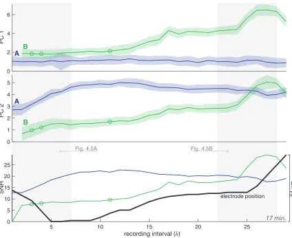
4.4 MHTC tracks, Session I . . . 79

4.5 Cluster sequence detail, Session I . . . 80

4.6 Hypothesis tree, Session I . . . 81

4.7 MHTC tracks, Session II . . . 82

4.8 Cluster sequence detail, Session II . . . 83

4.9 MHTC tracks, Session III . . . 84

4.10 MHTC tracks, Session IV . . . 85

4.11 MHTC tracks, Session V . . . 86

4.12 MHTC tracks, Session VI . . . 87

4.13 Rank of best global hypothesis, Sessions I–VI . . . 88

4.14 Nearest neighbor comparison (MAP clusters), Sessions I–VI . . . 89

(12)

5.1 Photograph of the miniature electrode microdrive with three commercial microdrives 92

5.2 Exploded view of electrode microdrive structure . . . 93

5.3 Photographs of the electrode microdrive . . . 93

5.4 Simultaneous recordings from the microdrive’s three electrodes . . . 96

5.5 Example neuron isolation by robotic microdrive (Isolation by IQM) . . . 97

(13)

List of Tables

2.1 Key Intervals Isolation Quality Metric . . . 21

3.1 Cluster Statistics of Selected Intervals . . . 45

3.2 Neuron Tracks . . . 46

(14)

Notation

Clustering

i indexes spike observations from the current interval g indexes cluster (mixture component), current interval j indexes cluster (mixture component), previous interval k indexes interval (discrete time step)

m indexes model class

Tk recording interval

∆ duration of recording interval

yi spike observation in feature space

d dimension of feature space dw dimension of full waveform space

N number of spike observations in current interval Yk _{set of spike observations on}_k_{th interval}

Y1:k _{set of all spike observations from intervals 1 to}_k

Mm model class

¯

M number of candidate model classes ηm number of parameters in Mm

Cg gth cluster in current interval

ng number of spike observations in clusterCg

Gm number of clusters (mixture model components) in Mm

Gmax maximal number of clusters considered by any model class ˆ

Gk−1 number of clusters identified on previous time step Θkm parameter set for mixture model classMm

π_gk mixture component weight θk

g mixture component density parameters

µkg mixture component mean

Σk

g mixture component covariance matrix

λk _{covariance volume}

zig spike–cluster membership indicators

Z set of all spike–cluster membership indicators (current interval) ζgj cluster–neuron association indicators

Z set of all cluster–neuron association indicators (current interval) ωk

j mixture component weight in prior

ψk

j mixture component density parameters in prior

S_jk−1 covariance matrix of prediction that prior mean is in same location

V observation volume

α forget factor

(15)

Hypotheses

k indexes interval or scan (discrete time step)

l indexes hypothesis

ρ(l) index of parent global hypothesis ofl m(l) index of parent model hypothesis of l g indexes measurements of a current interval j indexes targets in parent hypothesis

Mm model hypothesis

hl data association hypothesis

Hk

l joint hypothesis (particular model and data association)

H1:k

l global hypothesis through firstk intervals

Ωk all global hypotheses and observations at timek

τl set of assignments of measurements to existing targets underhl

νl set of measurements identified as new targets underhl

φl set of measurements identified as false clusters underhl

δj,l indicator of whetherjth target is tracked underhl

Nt number of active targets (tracks) in parent hypothesis

Nτ number of measurements from existing targets (under hl)

Nν number of measurements from new targets (underhl)

Nφ number of measurements from false clusters (underhl)

ˆ

Gm number of measurements inmth model hypothesis

Pd,j probability of detection of jth target

λν Poisson rate of new targets

λφ Poisson rate of false clusters

β minimum threshold for model class to become model hypothesis Kmiss number of missed detections before target is deleted

A data association matrix

agj elements of data association matrix

A∗ linear assignment cost matrix

Dynamical Model and State Estimation

xk

j state vector

ˆ µk

j measurement (cluster mean)

Fk state transition matrix

Hk measurement matrix

vk

j process noise

wk

j measurement noise

Qk

j process noise covariance matrix

Rk_j measurement noise covariance matrix xk_j|k−1 state prediction

Λk_j|k−1 state prediction covariance ˆ

µk_j|k−1 measurement prediction Sk

j innovation covariance

Kk

j Kalman gain

xk_j|k updated state estimate

(16)

Chapter 1

Introduction

This thesis presents new methods for classifying and tracking the signals of individual neurons in

extracellular neural recordings, as well as advances in a novel miniature robotic mechanism capable

of obtaining such recordings. These contributions will play a pivotal role in enabling an autonomous

neural interface, which, by frequent automatic repositioning of its recording electrodes, optimizes the

extracellular signals associated with individual neurons and maintains high-quality recordings for

long periods of time. Such autonomous movable electrodes may eventually overcome key barriers to

engineering a practical neuroprosthetic device and, in the near term, can significantly improve

state-of-the-art neuroscience experimental procedures. The remainder of this chapter provides further

motivation for this work, its problem statements and technical context, and an overview of the

contributions of subsequent chapters.

1.1

Motivation

1.1.1

Autonomous Neural Interfaces for Neuroprostheses

Recent progress in neuroscience has provided hope that paralyzed people may someday use thoughts

to control electromechanical devices such as robotic limbs to partially restore lost motor function

[1–4]. Such a device, termed a neuroprosthesis, could benefit patients with little other opportunity

for physically affecting their environment, such as those with severe spinal cord lesions or trauma,

neurodegenerative diseases such as amyotrophic lateral sclerosis (ALS), or stroke to motor cortex,

as well as those who have lost limbs. To accomplish this goal, a neuroprosthesis must perform

three distinct functions (Figure 1.1): obtain useful neural signals from the brain, decode the user’s

intentions from these signals, and control a mechanism (e.g., an actuated prosthetic arm) that carries

(17)

Courtesy Nicolas Hudson

Decode intended

action

Control external

device

Record neural

activity

Patrick J. Lynch 2006

Figure 1.1: Principal technical functions of a neuroprosthesis.

brain–machine interfaces (BMI)1.

While neuroprostheses have been demonstrated in several research labs, a critical barrier to

future practical neuroprosthetic devices now lies in the signal acquisition [5]. Scientifically, the most

desirable source of neural signals to control a neuroprosthesis, especially one with many degrees of

freedom, is the activity of individual neurons [1–4], orsingle units, which is obtained viaextracellular

recording. This activity is measured by microelectrodes inserted into the brain; for prostheses

patients, a robustneural interface with many electrodes must be surgically implanted in the brain

region(s) of interest and must operate for years at a time2_{. The goal of single-unit extracellular}

recording, more thoroughly described in Chapter 2, is to detect and localize in time the occurrence

of a neuron’s electrical impulses, termedaction potentials or spikes, which are the basis for neural

communication and information processing. It is widely accepted that the information output of a

neuron is encoded in the timing of its spiking activity, not in the shape of its spike waveforms, which

are highly stereotyped (see Figure 1.2). A successful extracellular recording, then, is one in which

the firing of spikes of individual neurons can be reliably detected and differentiated from other signal

sources; the neurons are then consideredisolated.

The timing of these spikes may then be analyzed for scientific studies or for control of a

neuro-prosthesis, decoding the intentions of a paralyzed user. In some brain regions, a strong correlation

may be observed between the activity of a neuron—often quantified as a firing rate of the number

of spikes over a short time interval (e.g., ∼80 ms)—and the subject’s concurrent or subsequent 1_{These terms are sometimes used interchangeably. In this thesis, a}_{brain–machine interface (BMI)}_{is broad term}

for a device that interacts with neural signals; aneuroprosthesiswill refer to a type of BMI that uses a brain-controlled mechanism to replace lost motor function (although the term is often used for sensory prostheses such as cochlear implants and motor prostheses attached to the peripheral nervous system); and the phrasebrain–computer interface (BCI)applies when the objective is to control a computer (e.g., a cursor on a screen) rather than a physically moving mechanism.

2_{Non-invasive recording techniques such as EEG, which records brain waves from electrodes placed on the scalp,}

(18)

physical motion. Often, this correlation relates to a certain direction of motion (or spatial location),

in which case we say the neuron is tuned to that direction (or location). For operation of a BMI,

a computer algorithm must first learn the tuning preferences of a collection of neurons during a

“training phase.” Subsequently, the user’s intentions may bedecoded from the observed firing rates

of these same neurons, provided the number of tuned units recorded is sufficient for “coverage” of the

physical region of interest. Thus, a successful neural interface must isolate many cells and maintain

these isolations of these neurons so that their previously calibrated characteristics may be used for

decoding commands.

Whether a cell is successfully isolated, and thus provides useful signals for the neuroprosthesis,

relies almost entirely on the effective placement of the uninsulated electrode tip with respect to

that cell body. In work related to this thesis, a robotic system has been proposed to autonomously

position electrodes so as to initially optimize and then maintain the quality of the recorded signal

over long periods of time [7–9]. This system consists of two parts: a mechanism, termed amicrodrive,

capable of independently positioning an electrode along a linear track with micron-scale precision,

and a hierarchical control algorithm to determine appropriate electrode movement commands. In

the algorithm’s main loop, the electrode’s signal is sampled for an interval of, say, 10 seconds, and

then analyzed to calculate the optimal electrode position adjustment.

Ultimately, the goal of this project is to build an array of many (perhaps one hundred)

inde-pendently actuated electrodes, each controlled by the autonomous positioning algorithm, all in a

package small enough to allow surgical implantation. Such a device offers the potential to overcome

many of the difficulties inherent in establishing the effective, long-lasting neural interfaces required

for practical neuroprostheses. Additionally, a robotic electrode paradigm can increase the quality

and efficiency of neuroscientific research techniques by eliminating the tedious manual process by

which electrophysiologists have traditionally optimized electrode placement. (The current state of

the autonomous electrode positioning system and a more detailed discussion of extracellular

record-ing procedures and challenges are provided in Chapter 2.)

1.1.2

The Spike Clustering and Neuron Tracking Problems

During extracellular recording, a single electrode’s signal may contain action potentials generated

by multiple neurons lying near the electrode tip. Because the goal of extracellular recordings is

to detect the activity of individual neurons, each detected spike must be associated to the neuron

that produced it (its generating neuron)—a task known as spike sorting. Typically, spike sorting

procedures classify the spikes according to waveform shape and amplitude; although the shape

of action potentials are very similar across neurons, the techniques assume that the separation

(19)

Spike Waveforms

Electrode Signal

PCA

Clustering

V

V 10 sec.

1.1 msec.

A

B

C

D

E

Figure 1.2: The spike clustering problem. (A) The electrode signal recorded over a particular intervalTk

may contain the spike waveforms of multiple neurons. (B) The spikes are extracted from the recorded voltage trace and aligned by their minimum and then (C) projected onto a feature space (here, the first two principal components). (D) In this space, the spikes of disparate neurons are “clustered” into sets. As will be conventional throughout this thesis, clusters are indicated with color and filled 2-sigma ellipses; black points indicate classification as “outliers.” Plot (E) shows the waveforms colored according to clustering results.

waveforms from the same neuron3.

Accurate spike sorting is critical, as the metrics from the signals of each distinct neuron are

vital both to electrode positioning, whose goal is to maximize signal quality, and to the scientific

or prosthetic uses of the recorded data, which generally rely on estimated neuronal firing rates

from the recordings. If spikes are incorrectly classified, these metrics may be severely corrupted.

Because of its importance and difficulty, spike sorting is typically achieved through a largely manual

process in neuroscience experiments, via visual examination of the spike waveforms. However, in

the autonomous electrode positioning algorithm introduced above, and for practical neuroprostheses,

spike sorting must be achieved in an unsupervised manner. Additionally, because the electrode signal

is sampled over many brief, successive recording intervals, not only must spikes be associated to their

generating neuron within a particular recording interval, but spikes from the same generating neuron

must be associated with each other across recording intervals. Thus, the ability to track individual

neurons over successive intervals is necessary for the algorithm to assess whether a change in electrode

position has improved the signal quality of these neurons.

Specifically, consider the following problem, illustrated in Figure 1.2. An electrode signal S is sampled over an interval T1 of length ∆. In a set of preprocessing steps, the spikes in S must be 3_{Note that the recorded signal is affected by the neurons’ varying distances from the electrode tip and the}

(20)

Consistent Clusters,

Neurons Tracked Inconsistent Clusters, Neurons Not Tracked

Recor

ding Interval

A B C A B C

A B C

?

Figure 1.3: The neuron tracking problem. In each recording interval, the current clusters must be matched to those in the preceding interval, thus propagating the identities of and associating all the spikes of persisting neurons. Four consecutive recording intervals of clustered neuronal spikes in a common PCA basis are shown. In the left column, three clusters are consistently identified in each recording interval; because each cluster appears in approximately the same location as in the last interval, the clusters are associated across intervals and carry forward the neuron IDs A, B, and C. In the right column, different clusters have been identified; the inconsistency of these clusters from one interval to the next complicates the tracking task, and the associations to clusters in the preceding interval are unknown.

detected, extracted from the voltage trace, and then aligned so that their waveforms may be more

readily compared. Then, the waveforms found in T1 are projected onto an d-dimensional feature space (e.g., a 2-dimensional principal component (PCA) basis; see Section 2.2.2.2) so that each

waveform is represented as a point. These points must then be grouped into sets via a clustering

procedure, where each cluster is assumed to be associated with a unique neuron in the multi-unit

signal.

Next, additional signal samples are taken across successive intervals T2, T3, and so on. After clustering results are computed for the intervalTk, each cluster in this interval must be associated

to a neuron that was previously identified in {T1, . . . , Tk−1}, or identified as a newly appearing

neuron not previously recorded. This tracking process, as illustrated by an example in Figure 1.3,

must be robust to changes and variability in the numbers, alignments, shapes, and amplitudes of

the neuronal signals over the recording. To reliably identify the signals of individual neurons across

successive sampling intervals, the clustering procedure must not only provide high quality results

within a sampling interval but also consistently identify similar clusters across sampling intervals so

that tracking is feasible.

The majority of this thesis addresses the above spike clustering and neuron tracking problems,

which are the critical challenges in the spike sorting process. (Previous work is leveraged for spike

(21)

compatible with many choices for these procedures.) To summarize, two data association challenges

must be faced: Classification orclustering refers to the process of grouping spike observations from

a single interval Tk into distinct sets, or clusters, effectively asserting that all the spikes in a single

cluster have arisen from the same neuron. Tracking is the procedure of associating clusters to each

other across recording intervals, identifying them as “belonging to” the same neuron—which, in

turn, assigns all the spikes associated with these clusters to a common generating neuron.

1.1.3

Other Applications

Although this work is primarily motivated by the needs of autonomous electrode positioning systems,

the spike sorting problem described above also arises in other electrophysiology applications. For

example, during the training phase of some brain–machine interfaces, multi-unit signals from each

electrode of an implanted static electrode array are sampled during repetitive execution of a task,

which typically lasts a relatively short duration (e.g., ∆ =∼5 sec.). In order to properly estimate the tuning properties of the neurons sampled by the array, the signal sources must be sorted on

each electrode and matched across each task execution. The neuronal properties learned during this

training phase may then be used during task execution of the BMI, provided the same neurons may

again be identified.

In multi-unit recordings gathered during basic electrophysiology experiments, automating the

spike sorting task can relieve this time-consuming burden from experimenters and perhaps even

improve the accuracy or the results, as manual sorting is known to be inconsistent [10]. For these

applications, it can be useful to divide lengthy recordings into short time intervals for spike sorting

and analysis, as the data are apt to be effectively stationary over these periods (see Section 2.3 and

Section 3.1 for more on non-stationarity). Here again, the neuronal signals must be clustered in each

analysis interval and then matched across intervals.

More generally, the fundamental clustering and tracking procedures addressed in this thesis are

not specific to electrophysiological data. Thus, the solutions presented here may be applicable to

other domains in which objects must be observed through probabilistically distributed groups of

measurements and tracked over successive “scans” or measurement intervals. Such problem

state-ments may occur in fields such as computer vision or other sensor processing disciplines.

1.2

Review of Existing Literature

This thesis builds upon work from several disparate domains: devices and algorithms for extracellular

recording and electrode positioning; spike sorting and, more generally, classification methods; and

target tracking. Existing literature from each domain is summarized below and reviewed more

(22)

While electrode microdrives have long been used for basic research in neurobiology, the system

introduced in [7–9] represents the first efforts to fully automate the process of extracellular recording

and in fact represents one of the first robots to operate autonomously within a primate brain for

extended periods of time. Previous attempts at automating small portions of the neuron isolation

process were reported by Fee [11], who demonstrated a method to stabilize intracellular recording

electrodes for a period of a few minutes, and by Baker et. al [12], who demonstrated a control

architecture for an acute microdrive that autonomously advances electrodes until target cells are

detected, at which point a human operator must optimize the recorded signal.

The electrode positioning algorithm requires a microdrive mechanism compatible with the

au-tonomous system paradigm and should be small enough for continuous use for days or even weeks

at a time4_{. Commercially available motorized microdrives are much too large to be practical for}

such semi-chronic use and generally require a subject to be restrained for the experiment’s duration.

While chronic implantable microdrives have been developed [13–17], these devices require manual

intervention to reposition the electrodes, such as turning lead screws. Muthuswamy et al. have

developed micro-machined actuators for implantable movable electrodes and have demonstrated a

prototype in an acute rat experiment [18]; however, it is unclear whether the high power

consump-tion and limited actuator range of their device will be appropriate for chronic setups in primates.

Also, an accompanying control algorithm would still be necessary, as it is not practical to require

constant human supervision to adjust the electrodes to achieve optimal signals.

A rich body of literature has addressed unsupervised classification, and many traditional

clus-tering procedures have been adapted to sort neural waveforms, including hierarchical [19], k-means

[20,21], neural networks [22], superparamagnetic [23], template matching [24], and density grids [25].

The optimization of a (typically Gaussian) mixture model [26] has been shown to be a particularly

effective approach in spike sorting [27–32]. However, most of these existing techniques are designed

for offline batch processing of large data sets, and no existing technique specifically addresses the

challenges of real-time processing of successive sampling intervals.

For such a recording scenario, the inconsistency of conventional clustering methods’ output and

the non-stationarity of the neuronal signals are the crucial issues, as each interval’s spikes are

clus-tered separately but must be matched to those in the preceding and subsequent interval(s) for neuron

tracking. Bar-Hillel et al. [32] are, to the author’s knowledge, the only others to explicitly address

these matters, but present a non-causal, computationally intensive method designed for offline

pro-cessing and hence not applicable to the real-time applications that motivate the work in this thesis.

Other authors have also characterized and addressed signal non-stationarity for single intervals of

long duration [33, 34], but these methods are not designed for the short, separate intervals discussed

4_{The origin of these requirements and their relationship to the fully implantable system suggested in Section 1.1.1}

(23)

here.

Although existing spike sorting techniques have seldom addressed the tracking problem described

in Section 1.1.2, an abundance of establishedmultitarget tracking (MTT) literature exists, primarily

intended for military and, more recently, computer vision applications (see [35] for a summary of

techniques). Most of these methods assume measurements of targets of interest are obtained in

suc-cessive “scans” of an observation volume, a scenario resembling the use of repeated sampling intervals

to track neurons [36, 37]. The key difference for the neuron tracking problem is that measurements

of the neuron’s “position” are actually obtained through groups of observations (clusters of spikes)

in every scan, whose associations are unknown5_{. In general, the tracking of objects observed by}

uncertain clusters of measurements is a novel problem addressed by this thesis.

Among the many target tracking techniques, a data association strategy called multiple

hypoth-esis tracking (MHT), attributed to Reid [38], is generally agreed upon as the preferred solution [39]

but is encumbered by computational infeasibility of the ideal implementation. From the

perspec-tives of this thesis, much of the recent target tracking literature falls into two categories: efforts to

formulate the MHT solution for a practical implementation even for large numbers of targets [40,41]

and increasingly sophisticated methods for scenarios such as maneuvering targets, nonlinear target

dynamics, or specific sensor types [37, 42]. The improvements in this latter category are generally

not necessary for the neuron tracking application, as models for neuron “dynamics” are typically

simpler and slower than those considered for modern tracking systems. Many techniques from the

former category may be useful for neuron tracking, although the numbers of neurons, or agents to

be tracked, are usually small compared to other target tracking applications.

1.3

Thesis Contributions and Organization

The remainder of this thesis is organized as follows. Chapter 2 provides further technical background

to contextualize the thesis’ contributions, specifically describing common techniques for extracellular

recording and previous work on the autonomous electrode positioning system. Additionally, it

further discusses the challenges inherent to extracellular recording to establish why the spike sorting

task is difficult.

In Chapter 3, a novel clustering method is developed, capable of overcoming many of these

challenges. Its strategy is based on the optimization of a Gaussian mixture model (GMM) via

expectation-maximization (EM) [26,43]. Assuming that the analysis of the data in the intervalTk−1 has yielded a reasonable clustering result, the model parameters estimated from intervalTk−1provide a Bayesian prior for the clustering of data in intervalTk. Thus, clustering is effected as a maximuma 5_{One may argue that, if only one spike for each neuron is observed at a time, the traditional tracking methods}

(24)

posteriori (MAP) method rather than maximum likelihood (ML) method. Additionally, the model’s

statistics from the preceding interval provide initial values (orseed clusters) for the EM computation.

Importantly, the method will likely succeed even if the preceding clustering was incorrect or if

different neurons’ signals are recorded during the two intervals. Not only does this procedure provide

more consistent clustering results, but it provides a simple neuron tracking solution “for free,” as it

quantifies the probability that a given cluster found in intervalTk is associated with a cluster found

in interval Tk−1. A Bayesian technique for choosing the best mixture model class is embedded in the approach as well.

A more sophisticated and robust solution to the tracking problem is presented in Chapter 4,

which incorporates the clustering procedure of Chapter 3 into a multiple hypothesis tracking (MHT)

framework. This approach is novel in its combination of clustering and tracking into a single solution,

tracking targets that may be observed only through collections of measurements from each recording

interval. Because the associations of these measurements (i.e., the clustering) is uncertain, multiple

“model hypotheses” for how an interval’s data may be clustered are maintained as well as the

standard data association hypotheses. The method, referred to asmultiple hypothesis tracking for

clusters (MHTC), fits naturally with the probabilistic theory and computations of the clustering

method described in Chapter 3.

Chapter 5 addresses the hardware required for the autonomous electrode positioning system,

reporting a novel electrode microdrive capable of semi-chronic use. This neural interface is the next

generation prototype of the microdrive presented in [7], which was the first specifically designed

for fully autonomous extracellular recordings. The advances in the robot described in this thesis

provide substantial improvements in terms of signal quality, robustness to biological environments,

experimental ease of use, and manufacturability. The microdrive is designed as a testbed for the

autonomous electrode paradigm and as a means to develop the specifications for future miniaturized

implantable devices. The current design is also immediately useful to the neuroscience research

community for longer-term electrophyisology experiments that cannot be carried out with currently

existing microdrives.

Finally, Chapter 6 summarizes the contributions of the thesis and suggests possible directions

(25)

Chapter 2

Background

This chapter provides context for the contributions of this thesis. First, since the thesis concerns

the acquisition and analysis of extracellular neuronal signals, the principal techniques and issues of

recording these signals are presented in Section 2.1, along with a description of the neurophysiological

environment. Second, Section 2.2 presents previous work on the autonomous electrode positioning

algorithm, in which the clustering and tracking methods are designed to operate and which controls

the electrode microdrive. Finally, several challenges that make spike sorting a difficult task are

discussed in Section 2.3.

2.1

Extracellular Recording: Environment and Techniques

The electrical impulses known as action potentials or spikes are the primary means of

informa-tion processing and transmission in the nervous system. Each nerve cell, or neuron, accepts input

principally via its dendritic tree, a set of branched projections that receive incoming signals from

other cells across connections known as synapses. This electrochemical stimulation is transmitted

to the neuron’ssoma, or cell body, and may trigger the neuron to fire an action potential of its own,

which will propagate out along itsaxon, a slender projection that carries the action potential toward

downstream neurons. It is believed that the connectivity of neurons determines how information

is processed and stored, and that particular neurons have particular functions or associations to

particular memories, sensory processes, motor commands, etc. [44].

The goal ofextracellular single-unit recording is to detect the spikes of individual neurons1_.

Sci-entific experimenters may then examine the timing (e.g., firing rate) of each unit’s action potentials

to infer, for example, the role of the neurons in a particular brain region or the connectivity of larger

brain structures. When used for brain–machine interfaces (BMIs), as described in Section 1.1.1, the

1_{Other useful signals may also be obtained from extracellular electrodes.} _The_{local field potential (LFP)}_{, for}

(26)

neurons’tuning may first be learned and then used to guide the BMI.

These extracellular recordings are made by inserting electrodes, typically sharpened metal wires

insulated along their length and exposed at the tip2_{, into neural tissue to measure the electrochemical}

disturbance in the extracellular medium caused by a neuron’s action potentials3_{. The tip of a}

recording electrode must generally lie within about 50 µm of the neuron’s soma to be able to discriminate these disturbances, which are usually 100 µV or less, above the background of gross neural activity and measurement noise. This requirement defines a “listening sphere” around the

neuron (see Figure 2.1C), and a closer proximity may be required to sufficiently distinguish the

signals of different neurons [46, 47]. Each neuron cell body is approximately 10–50 µm wide and generally the signals of a maximum of about four units may be discernible on the electrode’s signal at

any given time (though the actual cell density within 50µm may be significantly greater) [9, 48]. As summarized below, extracellular recordings can be carried out in anacute or in achronic manner.

The autonomous electrode positioning system introduced in Section 1.1.1, and thus the contributions

of this thesis, can benefit both types of extracellular recordings.

Figure 2.1: Extracellular recording environment and example signals: cross-sectional diagrams of (A) acute and (B) chronic recording setups; (C) detail drawing of recording site at electrode tip; (D) 10-second filtered signal sample from an electrode, with (E) the action potential (spike) waveforms extracted from the recording and aligned by their minimum.

2_{Silicon shafts with electrically active recording sites along their shanks may also be used [45].}

3_{This technique may be contrasted to} _{intracellular recording}_{, in which the electrode is placed inside a neuron}

(27)

2.1.1

Acute Recordings

In acute recordings, which are primarily used for scientific research, electrodes are inserted and

removed from the neural tissue during each recording session (which typically lasts a few hours). To

enable these recordings in cortex, a portion of the skull over the brain region of interest is typically

removed and replaced with a sealable cranialrecording chamber (see Figure 2.1A); for example, a

16-mm inner-diameter cylindrical recording chamber is a standard used in the neuroscience co16-mmunity.

During an acute recording session, a microdrive4_{, affixed to the opened chamber, is used to lower one}

or more electrodes into cortical tissue and then subsequently finely position the electrodes. Electrodes

are advanced through neural tissue along a straight line, with the position of each electrode described

by its depth along this linear track. Note that linear movement of the electrode through tissue

substantially reduces the amount of tissue damage relative to possible curvilinear motion of the

electrode tip; if one wishes to interrogate a 3-dimensional volume of neural tissue, multi-electrode

devices are employed in an arrayed geometry.

While the electrode movement is typically motorized, the electrode’s motion is at present

manu-ally determined by the experimenter. The process of determining the exact position of each electrode

is commonly guided by the use of visual (oscilloscope) and auditory (loudspeaker) representations of

the voltage signal, and the experimenter relies on experience and intuition to determine proper

elec-trode placement. The elecelec-trode must be close enough to the neuron for a high quality recording, yet

far enough away to avoid damaging it. During the course of a typical experiment, the experimenter

must monitor the electrode and often reposition it to account for tissue decompression effects.

Sort-ing the spikes of different neurons may be achieved manually in real time usSort-ing commercial software

aids or may be deferred for later offline processing of the entire recording session. The process of

isolating and maintaining high quality neuronal signals thus consumes a significant amount of the

experimenter’s time and focus.

Simultaneous recordings with many electrodes are becoming an increasingly important technique

for understanding how local networks of neurons process information, as well as how computations

are coordinated across multiple brain areas. Commercial microdrives with sixteen or more electrodes

are now available [12]. As the number of electrodes increases, the manual task of positioning each

electrode to maintain a high quality neuronal signal becomes intractable for a single experimenter.

Data collection in these experiments is essentially limited by how many channels an experimenter can

effectively monitor—most experimenters agree that about three or four electrodes is the maximum

that can be juggled effectively by an experienced electrophysiologist. Thus, by continually monitoring

the signal and automating the process of placing and repositioning electrodes, an autonomous system

4_{Recall that a microdrive is an electromechanical device that can position an electrode along a linear track with}

(28)

can significantly improve the efficiency and quality of acute multi-electrode studies.

2.1.2

Chronic Recordings

In chronic recordings, multi-electrode assemblies with fixed geometry, which typically consist of

bundles of thin wires or arrays of silicon probes, are surgically implanted in the region of interest

[45, 49–51] (see Figure 2.1B) and remain in place for weeks, months, or possibly years at a time.

Such chronic implants enable investigations of larger populations of neurons and can be used as the

front end of a neuroprosthesis or for longer-term scientific studies.

Current chronic recording technology suffers from a number of limitations. The implant’s signal

yield (the percentage of the array’s electrodes that can record a useful signal) depends largely upon

the luck of the initial surgical placement. Because it is generally impossible for all of the implanted

electrode tips to fall within the “listening sphere” of an active neuron, not all of the implanted

electrodes will provide a useful signal. Moreover, blood pressure variations, breathing, and small

mechanical shocks can cause migration of the electrodes in the tissue, leading to further degradation

of the signal [11, 52]. Finally, reactive gliosis can encapsulate the electrode, diminishing signal

quality over time [53]. All of these effects conspire to limit the usefulness and practical longevity of

chronically implanted electrode arrays.

A chronic array whose electrodes can be continually repositioned after implantation may

over-come many of these limitations. With such an implant, the overall signal yield can be improved

by moving the electrodes to optimal neuronal recording sites. Further, neurons whose activity is

well correlated with the objectives of the neuroprosthesis could be specifically sought, thus

provid-ing more information per electrode channel than static arrays. Movprovid-ing electrodes may also enable

recording in brain regions that are not easily accessible, such as those within a cortical sulcus (a

fissure resulting from the folded nature of the cerebral cortex).

Commercially available motorized microdrives are much too large to be practical for chronic

use and generally require a subject to be restrained for the experiment’s duration. While chronic

implantable microdrives have been developed [13–17], these devices require manual intervention

to reposition the electrodes, such as turning lead screws. Muthuswamy et al. have developed

implantable actuated electrodes and have demonstrated a prototype in an acute rat experiment [18].

However, it is unclear whether the high power consumption and limited actuator range of their

device will be appropriate for chronic placement in primate brains. Also, an accompanying control

algorithm with automated spike sorting and electrode positioning would still be necessary, as it is not

practical to require constant human supervision to adjust the electrodes to achieve optimal signals.

The algorithms and experimental demonstrations described in the next section provide the

foun-dation for future generations of chronic “smart” implantable multi-electrode systems. Although new

(29)

for initial attempts at developing miniaturized, biocompatible, actuated electrodes that would enable

a compact, implantable implementation of this approach), the small size of the microdrive described

in Chapter 5 allows it to serve as a testbed for these future devices.

2.2

Autonomous Electrode Positioning Algorithm

This section summarizes prior relevant work aimed at creating a control algorithm for autonomous

electrode positioning in extracellular recordings [7–9]. The control algorithm utilizes a hierarchical

closed loop approach to determine, based on the recorded signal and the electrode’s position history,

the best depth for each electrode. The goal is to place each electrode so that the spikes from an

isolatedneuron can be unambiguously detected in the noisy voltage recording and discriminated from

the signals of other nearby neurons. This section presents the control system structure and then

describes its individual components in more detail. Because each electrode is moved independently,

only the processing steps for a single electrode need to be considered; these steps are run in parallel

for each electrode in a multi-electrode microdrive.

2.2.1

Control System Structure

The control algorithm operates in a cycle, illustrated in Figure 2.2. Let these cycles be indexed

by the integer k, k = 1,2, . . .. The cycle begins with sampling the electrode signal over a short sampling interval (denoted byTk, which is typically of duration 10–20 seconds) while the electrode

is stationary, followed by analysis of this signal to determine if and how the electrode should be

repositioned, and ending with the movement of the electrode to a new position (if necessary).

A hierarchical control algorithm determines the electrode movement commands. The inner-most

loop of this algorithm (Section 2.2.3) attempts to isolate an individual neuron by optimizing the

quality of the recorded signal via small local movements of the electrode tip, assuming that the tip is

close enough to a neuron for the isolation process to be possible. The outer control structure consists

of a finite state machine supervisory controller (Section 2.2.4) which has several purposes. First,

it manages the neuron isolation process: It moves the electrode until a region of sufficiently strong

neuronal signal sources is found and then further searches this region to acquire the information

needed to initiate the isolation procedure. Additionally, the supervisory system handles several of

the complicating realities of the extracellular recording process. Of course, to provide useful

neu-ronal signal metrics from the electrode recording, these algorithms require several signal processing

steps, which most critically include spike sorting, motivating Chapters 3–4 of this thesis. Most of

these processing tasks have traditionally been performed manually in electrophysiology experiments;

producing automated and unsupervised methods presents significant challenges in addition to those

(30)

Electrode Positioning

Algorithm Cycle

1

2

4

5

6

3

Record Data

Detect

Spikes & TrackCluster

Compute Metrics

Decide Motion Move

Electrode

V

V PCA

electrode depth

SNR

SNR Curve

Figure 2.2: Autonomous electrode positioning algorithm cycle. Plots show key data involved at each step of the cycle. During thekth cycle: (1) A short data sample (voltage trace) is recorded during intervalTk, from

which (2) spike waveforms are detected, extracted, and aligned. (3) Using their PCA representations, these spikes are clustered by their generating neurons and associated with the neurons recorded on the previous cycle. (4) SNR and IQM metrics are computed and then (5) used to determine the electrode motion commands to optimize the SNR curve. (6) Finally, the electrode is moved to its commanded position.

2.2.2

Signal Processing and Metrics

2.2.2.1 Spike Detection

The first step of unsupervised signal processing on the electrode’s recorded voltage trace is spike

detection, which identifies the action potential events in the raw electrode signal of intervalTk. We

employ a wavelet-based method developed by Nenadic and Burdick [55] specifically designed for this

application. By projecting the electrode signal onto a specially designed wavelet basis, spike-like

waveforms can be detected in the raw signal, and short intervals (∼1.1 ms in length) of the signal centered on the putative spike occurrence are extracted (see Figure 2.1D and E). All of the spike-like

waveforms found duringTk are temporally aligned by their waveform minima in preparation for the

(31)

2.2.2.2 PCA and Other Feature Spaces

If each extracted waveform containsdwvoltage samples (e.g.,dw= 23 for a 1.1 ms interval sampled

at 20 kHz), then each waveform xi may be considered a vector in dw dimensions (i.e., xi ∈ Rdw_). Drastically reducing the dimension of the spike waveform representations to ddw dimensions is

computationally preferred for most spike sorting procedures, and this step may often be accomplished

without losing much of the discriminability information contained in the waveforms. Dimensionality

reduction is accomplished by selecting highly informativefeaturesof the waveforms and using them as

the basis in which spike sorting operates; an early feature space, for example, consisted of waveform

amplitude and a measure of its width.

The use of a 2-dimensional principal component analysis (PCA) basis is common practice in

spike sorting [27]. Let {wj} be the eigenvectors of the sample covariance matrix5 of all waveforms

{xi}detected in interval Tk, and let these eigenvectors be ordered from greatest to least eigenvalue

λj. Then the firstdeigenvectors (called theprincipal components orPCs) form the d-dimensional

PCA basis; the feature space spike representation may be calculated by yi = WTxi, whereW =

[w1w2. . . wd] [56]. Geometrically, the first principal component is the direction of largest variance

in {xi}, the second PC is the direction orthogonal to the first PC with largest variance, and so on;

the features{yi}are the projections of{xi}onto the space defined by the PCs. PCA representations

typically capture 70% or more of the spike waveform variance. Several other choices of feature space

are possible and are later discussed as an area of future investigation.

2.2.2.3 Spike Clustering and Neuron Tracking

The spike sorting task of clustering the spikes according to their generating neuron and tracking the

neurons across successive recording intervals comes next. This is the primary topic of Chapters 3–

4 of this thesis. Before the contributions presented in those chapters were developed, the control

algorithm was tested with a clustering technique based on maximum likelihood (ML) optimization of

a Gaussian mixture model [57]. No attempt to explicitly track the neurons across sampling intervals

was implemented.

2.2.2.4 Signal and Isolation Quality Metrics

After the spikes have been processed as above, two signal metrics are calculated for the neurons

identified in intervalTk:

• A signal quality metric (SQM) determines the general quality of the extracellular signals

as-sociated with a particular neuron.

5_{The sample covariance of the points}_{_x

i}Ni=1is Σ = 1 N−1

PN

(32)

• An isolation quality metric (IQM) measures the separation of one neuron’s waveforms from

those of other neuronal signals that appear in the same recording interval.

The SQM is the algorithm’s main target, and the dominant neuron is chosen as the one whose

signals have the highest average SQM. This is the neuron whose signal is to be ostensibly optimized

by the electrode’s movements. The signal-to-noise ratio (SNR) will here be assumed to be the signal

quality metric, although other choices of SQM are possible (see [9] for examples). In this application,

the SNR is defined as the mean peak-to-peak amplitude of the neuron’s waveforms detected in Tk

divided by the RMS amplitude of a spike-free noise sample taken during intervalTk.

Because a neuron’s signal is only valuable if it can be distinguished from those of surrounding

neurons, the IQM provides a measure of “isolation” of the waveforms of the dominant neuron from

other detected spikes. The IQM is based on theisolation distance (ID) [58], which, for clusterCg

containingNg spike samples, is defined as the Mahalanobis distance between its center µg and the

Ngth closest spike not in clusterCg (denoted byyj):

IDg=

q

(yj−µg)TΣg−1(yj−µg).

That is, the ID is the radius of the smallest ellipse (with shape defined by Σg) containing all the

spikes in cluster Cg and an equal number of spikes not in cluster Cg (in effect, a measure of the

“moat” around cluster Cg). In practice, the noise sample observations are included here as well,

handling the case when one neuron has generated more than half of the spikes duringTk. Note that

the SQM is calculated from the spike waveforms, while the IQM is computed in feature space (PCA

basis). A thorough discussion of different neuronal signal metrics and their uses is documented in [9].

2.2.3

The Isolation Control Loop

Assume for now that in the current interval Tk the signal from the dominant neuron is sufficiently

strong. Based on the processed neural data and the quality metrics just defined, the isolation control

loop determines if repositioning the electrode can improve the signal quality of the dominant neuron.

In the idealized scenario where the dominant neuron’s signals may be consistently tracked from one

recording interval to the next, and are ever present, the algorithm commands the electrode motion

solely to increase the SNR of that neuron as outlined below.

Detailed computational models [8] of the extracellular field generated around a typical cortical

pyramidal neuron show that when the electrode tip is within the “listening sphere” of a neuron,

the variation of the neuronal signal’s SNR with respect to electrode position traces out a unimodal

(33)

signals are highly noisy, the metric R should be considered a random variable with an associated regression functionM(u) =E[R|u], whereE[· | ·] denotes conditional expectation. This regression function isa priori unknown, except that it has a unimodal shape. Only noisy observations of the

SNR, obtained via the preprocessing steps summarized above, are available. In order to optimize the

SNR using only the available noisy samples, the isolation process adaptively estimates the regression

function (the smoothed SNR curve), and the electrode’s movements are chosen to seek the extremal

point of the adaptively evolving SNR curve.

The regression function model M(u) is assumed to be a linear combination of basis functions: M(u, mk, Bk) =P

mk

i=1bi,kψi(u), wheremk is the number of basis functions employed during cyclek

andBk= [b1,k, b2,k, ... , bmk,k]

T _{are the corresponding expansion coefficients. The model parameters}

Bk and model complexitymk must be estimated from the SNR observations and adaptively updated

as new data become available. For a given model estimate, the electrode’s next position, uk+1, is determined as:

uk+1=uk+C|Hk|−1 ξk , (2.1)

where C >0 is an appropriately chosen scale factor andξk and Hk are respectively the estimates

of the first and second derivatives of the regression function at the electrode’s current position,uk.

Note that Eq. (2.1) represents a stochastic version of Newton’s method. Convergence of the electrode

position to the maximum of the SNR curve is considered attained at iterationk∗ifC|Hk∗|−1ξ_k∗< , where is a tolerance chosen by the user. The position uk∗ is then declared the optimal electrode placement, whereupon the finite state machine supervisory controller transitions to a “maintain”

mode (see Section 2.2.4). The regression function M(u), from whichξk and Hk are determined, is

estimated as follows.

While many basis function choices are possible, polynomial bases can sufficiently capture the

ge-ometry of unimodal SNR curves (see [8]) and greatly simplify the estimation process. For polynomial

bases, the regression function afterkiterations is

ˆ

M(u, mk, Bk) = mk X

i=1

bi,ku(i−1).

Let {u1, u2, ... , uk} be a sequence of (electrode) positions with the corresponding SNR samples

denoted R1:k = {r(u1), r(u2), ... ,r(uk)}. At each electrode location uj (j = 1,2, ... , k),

multi-ple observations of SNR have been taken (one for each isolated neuronal waveform), i.e., r(uj) =

r1(uj), r2(uj), ... , rnj(uj) T

, where nj is the total number of observations atuj (this number may

vary across sampling intervals).

Determining the “correct” number of basis functions, mk, amounts to model selection problem.

(34)

order of the model that is most probable in view of the dataR1:k and any prior information,I. The

probability of the model ˆMmk givenR1:k andI follows from Bayes’ theorem

P( ˆMmk| R1:k, I) =

p(R1:k|Mˆmk, I)P( ˆMmk|I) p(R1:k|I)

mk = 1,2, ... , Nmax, (2.2)

where ˆMmk is short for ˆM(u, mk, Bk) with fixedmk. Here, I represents the model selection result obtained in the previous intervalTk−1—the posterior P( ˆMmk−1| R1:k−1, I) calculated at iteration (k−1) can be used as the prior at iterationkin Eq. (2.2). The recursion is initialized with a uniform prior densityP( ˆMmk0|I) =

1

mmax, where k0 denotes the smallest admissible number of iterations, below which there is an insufficient amount of data to reliably model the regression function. The

model order is chosen to maximize the posterior probability (2.2), i.e.,

m∗_k= arg max 1≤mk≤mmax

P( ˆMmk| R1:k, I) k=k0, k0+ 1, ... .

To perform this maximization, the posterior P( ˆMmk| R1:k, I) of each candidate model ˆMmk must be evaluated by marginalizing the unknown parametersBk. With a Gaussian noise assumption and

polynomial bases, the marginalization ofBk can be performed analytically [8].

Once the optimal model orderm∗_kat timekis known, the parameters of the model ˆM(u, m∗_k, Bk)

are estimated by a linear least-squares method:

B_k∗= arg min

Bk   

k

X

j=1

kΨj,kBk−r(uj)k2

  

k=k0, k0+ 1, ... ,

where the matrix Ψj,k ∈Rnj×m∗k consists of n_j identical rows given by [1, u_j,· · · , u(m ∗ k−1)

j ]. Once

the optimal parametersB_k∗ are estimated, the optimal model ˆM_k∗(u)≡Mˆ(u, m∗_k, B∗_k) at iterationk is fully specified. From this result the gradient and Hessian of the optimal model are then used in

Eq. (2.1) to determine the electrode movement.

Because sudden large electrode movements are unacceptable, the maximum step size is limited

by a constant ∆max, chosen before the experiment. This is especially useful for iterations where the

optimal model is found to be a straight line (m∗_k = 2), which results inHk = 0 and infinitely large

step size in Eq. (2.1). Likewise, if for somek > k0we obtain ˆMk(u) =b₁∗_,k, i.e.,m∗_k= 1, thenξk = 0

and the recursion (2.1) breaks. In this case the algorithm uses a simple control strategy:

uk+1=uk+ ∆sample,

(35)

2.2.4

Finite State Machine Supervisory Controller

To manage the basic neuron isolation process, while also accounting for many additional challenges

of practical extracellular recording, a finite state machine architecture guides the overall electrode

movement process. This system is termed thesupervisory finite state machine(SFSM). During each

algorithm cycle, the electrode movement decision (immediately following the signal acquisition and

analysis steps) depends on the current state of the SFSM, with individual states and state transitions

crafted to guide behavior appropriate to seeking and isolating neurons. A prototypical pathway of

state transitions is described below to describe the most common issues and SFSM operation; for

more details, see Branchaud’s thesis [9].

When electrodes are first lowered into neural tissue, the electrode tip may not lie in electrically

active tissue. The SFSM initiates in theSpike Searchstate (see numbered states in Figure 2.3), whose

goal is to find an electrically active tissue region. In this state, the electrode moves in increments

of ∆search (∼20 µm) until a sufficient number of spikes are detected in interval Tk (according to

a minimum firing rate set before the experiment), at which point the SFSM transitions to the

Gradient Search state. TheGradient Search state seeks to determine if a viable SNR curve can be

constructed. Observations of the SNR are made at regular intervals of ∆sample (∼10µm) until k0 observations are completed (typically, k0 = 3 is used), at which point the optimization procedure of Section 2.2.3 determines the most likely orderm∗_k that fits the SNR observations. As described above, ifm∗_k = 1 the electrode continues in steps of ∆sample(the SFSM stays inGradient Search). If m∗_k >1, indicating that a potentially viable SNR curve has been found (i.e., there is a high likelihood that a nearby neuron can be isolated), the SFSM transitions toIsolate Neuron.

As long as the SFSM remains inIsolate Neuron, the algorithm described in Section 2.2.3 operates,

updating the SNR curve with the new observations and moving the electrode toward the estimated

maximum. When the maximum of the SNR curve is reached, the SFSM state transitions toNeuron

Isolated, but only if certain IQM conditions are also met (see below).

In Neuron Isolated, the electrode generally remains stationary while the SNR is continually

monitored over successive sampling intervals. Often, the dominant neuron will drift away from the

electrode, causing a decrease in the SNR. When the SNR drops below a percentage (typically 85%)

of its value at the original isolation, the SFSM transitions to Re-Estimate Gradient in an attempt

to reposition the electrode to maintain the high quality isolation. In the Re-Estimate Gradient

state, the electrode is moved in increments of ∆resample (∼5 µm) to find a new gradient now that the dominant neuron has likely drifted away. In this state, the electrode is retracted, as the most

common neuron drift is due to tissue decompression and is directed up towards the electrode. Once a

new gradient is found, a transition is made toRe-Isolate Neuron, where the optimization procedure is

again used to isolate the neuron. If, at any time in theRe-Estimate Gradient orRe-Isolate Neuron

(36)

Spike

Search GradientSearch NeuronIsolate

Neuron Isolated

Re-Estimate

Gradient Re-IsolateNeuron Spikes

Detected DetectedGradient

Maximum Found

Signal Reclaimed Signal

Degrades

Gradient Detected

Maximum

Found _AwayBack

Neuron Isolated

Spike Search

Max. SNR Reached No Spikes

Detected 4

1 2 3

5 6

ISOLATE

RE-ISOLATE

IQM

[any state] [any state]

[any state] Cannot Isolate

WAIT

WAIT WAIT

WAIT

Figure 2.3: The supervisory finite state machine (SFSM). Transition criteria are noted between states. States are grouped into three modes (Isolate, Isolated, and Re-Isolate) for convenience. Transitions with

Waitmust meet transition criteria inR consecutive cycles, reducing sensitivity to transients. Transitions on the right may be made from any state.

declaration, theNeuron Isolated state is restored.

The isolation quality metric (IQM) plays a strong role in governing the SFSM state transitions,

summarized in Table 2.1. SNR is a good metric to indicate the overall signal strength and

relia-bility but is insufficient for jud

Target tracking using clustered measurements, with applications to autonomous brain-machine interfaces