EARTHQUAKE ENGINEERING RESEARCH LABORATORY
SEMI-ACTIVE CONTROL OF DYNAMICALLY EXCITED
STRUCTURES USING ACTIVE INTERACTION CONTROL
BY
YUNFENG ZHANG
REPORT
No.
EERL 2001-01
A REPORT ON RESEARCH PARTIALLY SUPPORTED BY
KAJIMA CORPORATION AND THE EARTHQUAKE RESEARCH AFFILIATES
PROGRAM OF THE CALIFORNIA INSTITUTE OF TECHNOLOGY
PASADENA, CALIFORNIA
AND THE EARTHQUAKE RESEARCH AFFILIATES PROGRAM OF THE CALIFORNIA
Using Active Interaction Control
Thesis by
Yunfeng Zhang
In Partial Fulfillment of the Requirements
for the Degree of
Doctor of Philosophy
California Institute of Technology
Pasadena, California
2001
©
2001Yunfeng Zhang
Acknowledgements
I would like to express my sincere appreciation to my advisor, Professor W. D. Iwan, for
his guidance and encouragement during the course of my graduate study at Caltech. I
consider myself fortunate for having the opportunity to share some of his knowledge and
experience. My sincere gratitude also goes to other faculty members in Thomas Building
for their helpful suggestions on this research. In particular, I wish to thank Professor James
L. Beck and Professor John F. Hall for their encouragement and assistance in my graduate
study at Caltech.
I am also grateful to Caltech for the excellent education and financial assistance which
I received during my graduate study. I also express my gratitude to the Kobori Research
Complex of the Kajima Corporation which has provided partial support for this
investiga-tion.
I also want to extend my thanks and best wishes to all my fellow students and friends in
Thomas Building. With their presence and companionship, my graduate study at Caltech
has been made most enjoyable.
Finally, I want to express my deep gratitude and love to my wife, Hongmei, for her
Abstract
This thesis presents a family of semi-active control algorithms termed Active Interaction
Control (AIC) used for response control of dynamically excited structures. The AIC
ap-proach has been developed as a semi-active means of protecting building structures against
large earthquakes. The AIC algorithms include the Active Interface Damping (AID),
Opti-mal Connection Strategy (OCS), and newly developed Tuned Interaction Damping (TID)
algorithms. All of the AIC algorithms are founded upon the same basic instantaneous
op-timal control strategy that involves minimization of an energy-based performance index at
every time instant.
A typical AIC system consists of a primary structure targeted for vibration control, a
number of auxiliary structures, and interaction elements that connect the auxiliary
struc-tures to the primary structure. Through actively modulating the operating states of the
interaction elements according to pre-specified control logic, control forces favorable to the
control strategy are reactively developed within the interaction elements and the vibration
of the primary structure is thus restrained. The merits of this structural control approach
include both high control performance and minimal external power requirement for the
op-eration of the control devices. The latter is important during large earthquakes when power
blackouts are likely to occur. Most encouraging is that with currently available technology
this control approach can be readily implemented in real structures.
In this thesis, the cause for an over-attachment problem in the original OCS system is
clarified and corresponding counter-measures are proposed. The OCS algorithm is
refor-mulated within an energy framework and therefore all of the AIC control algorithms are
unified under the same instantaneous optimal control strategy.
To implement the AIC algorithms into multi-degree-of-freedom systems, two approaches
are formulated in this thesis: the Modal Control and Nodal Control approaches. The Modal
Control approach directs the control effort to certain dominant response modes, and the
Nodal Control approach directly controls the response quantities in physical space. It is
found that the Modal Control approacli is more efficient than the Nodal Control approach.
results for three-story, nine-story and twenty-story steel-framed buildings. The statistical
Contents
Acknowledgements
Abstract
1 Introduction
1.1 Background and Motivation
1.2 Scope and Organization of the Thesis
2 Active Interaction Control of Linear SDOF Systems
2.1 Introduction . . . .
2.2 Assumptions and Formulation .
2.3 Interaction Elements . . . .
2.4 Control Strategy and Stability
2.5 Idealized AID and OCS Models
2.5.1 Idealized SDOF AID Model .
2.5.2 Idealized SDOF OCS Model .
2.6 Optimal Connection Strategy and Tuned Interaction Damping
2. 7 Numerical Study and Discussion . . . .
2.7.1 Idealized Case: Free Oscillation .
2. 7 .2 Seismic Excitation . . . .
2.8 Effects of Sampling Period and Time Delay
2.8.1 Control-Sampling Period.
2.8.2 Time Delay . . . . . .
3 Active Interaction Control of Linear MDOF Systems
3.1 Introduction . . . .
3.2 Model Formulation
3.3 Control Force . . . .
3.3.1 Top (N'h) Floor
iii
iv
1
1
6
8
8
9
11
12
17
17
18
19
24
25
25
29
29
30
61
61
62
64
3.3.2 Other (i'h) Floors (i = 1, ... , N-1)
3.4 Modal Control
3.5 Nodal Control .
3.6 Building Models and Design Procedure .
3.6.1 General Design Procedure for AIC System .
3.6.2 Outline of a 3-story Building Model
3.6.3 Outline of a 9-story Building Model
3.6.4 Outline of a 20-story Building Model .
3. 7 Numerical Study and Discussion .
3.7.l The 3-story Building Model
3. 7.2 The 9-story Building Model
3. 7. 3 The 20-story Building Model
3.7.4 The High Viscous Damping System
4 Statistical Behavior of Active Interaction Control Systems
4.1 Introduction . . . .
4.2 Simulation of Earthquake Ground Motions .
4.3 Statistical Performance of AIC Systems
4.4 Parametric Study . . . .
4.4.1 Stiffness Ratio a
4.4.2
4.4.3
4.4.4
Frequency Ratio 'I/;
AS Damping Ratio (2
Control Force Limit Ratio 'TJ •
5 Conclusions and Future Research Directions
5.1 Summary .
5.2 Conclusions
5. 3 Future Research Directions
Bibliography
A Partitioned Predictor-Corrector Method
B Analysis of Two Simple Cases
B.0.1 Free Oscillation . . . .
B.0.2 Harmonic Excitation .
C Finite Element Models of the 9- and 20-story Buildings
153
154
170
List of Figures
1.1 A Building with AVS Control Device .
2.1 Schematic of an AIC System Model
2.2 Schematic of Interaction Elements .
2.3 Response Time Histories of the PS Controlled by the Two OCS Algorithms 5
32
32
Under ELC Ground Motion . . . 33
2.4 Response Time Histories of the PS and AS Controlled by the OCS Algorithm
Under Harmonic Excitation . . . 33
2.5 Attachment Number and Normalized Displacement vs. AS Damping Ratio
of the OCS System Under Harmonic Excitation (thick line = Attachment
Number, thin line = Normalized Displacement Response of the PS, a =
Stiffness Ratio, (3
=
Mass Ratio, Texc=
Forcing Frequency) . . . 342.6 Response Time History of a Harmonically Excited OCS System with AS
Parameters: (2 = 603, (3 = m2/m1 = 0.1 . . . 35
2.7 Response Time History of the AID, OCS with Undamped AS, OCS with
Damped AS, and TID Systems Under Harmonic Excitation . . . 35
2.8 Attachment Number Time History of the AID, OCS with Undamped AS,
OCS with Damped AS, and TID Systems Under Harmonic Excitation . . . 36
2.9 Hysteresis Diagrams of the AID, OCS with Undamped AS, OCS with Damped
AS, and TID Systems Under Harmonic Excitation 36
2.10 Schematic of Two Configurations of AIC Systems . 37
2.11 Displacement Time History of AIC System in Free Vibration 37
2.12 Hysteresis Diagram of AIC System in Free Vibration, Type 1 Configuration 38
2.13 Accelerograms of Four Historical Earthquakes: (a) El Centro (b) Hachinohe
(c) Northridge (d) Kobe . . . 38
2.14 Displacement Time Histories of the Controlled PS Excited by the ELC Ground
2.15 Velocity Time Histories of the Controlled PS Excited by the ELC Ground
Motion, Type 1 Configuration . . . 39
2.16 Acceleration Time Histories of the Controlled PS Excited by the ELC Ground
Motion, Type 1 Configuration . . . 40
2.17 Displacement Time Histories of the AS Excited by the ELC Ground Motion,
Type 1 Configuration . . . 40
2.18 Acceleration Time Histories of the AS Excited by the ELC Ground Motion,
Type 1 Configuration . . . 41
2.19 Attachment Time Histories of the AID, OCS, and TID Systems Excited by
the ELC Ground Motion, Type 1 Configuration . . . 41
2.20 Hysteresis Diagram of the AID, OCS, and TID Systems Excited by the ELC
Ground Motion, Type 1 Configuration . . . 42
2.21 Displacement Time Histories of the PS Controlled by the AID, OCS, and
TID Algorithms Excited by the HAC Ground Motion, Type 1 Configuration 42
2.22 Velocity Time Histories of the PS Controlled by the AID, OCS, and TID
Algorithms Excited by the HAC Ground Motion, Type 1 Configuration . . 43
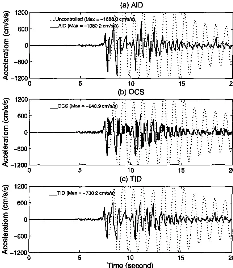
2.23 Acceleration Time Histories of the PS Controlled by the AID, OCS, and TID
Algorithms Excited by the HAC Ground Motion, Type 1 Configuration . . 43
2.24 Displacement Time Histories of the AS Controlled by the AID, OCS, and
TID Algorithms Excited by the HAC Ground Motion, Type 1 Configuration 44
2.25 Acceleration Time Histories of the AS in the AID, OCS, and TID Systems
Excited by the HAC Ground Motion, Type 1 Configuration . . . 44
2.26 Attachment Time Histories of the AID, OCS, and TID Systems Excited by
the HAC Ground Motion, Type 1 Configuration . . . 45
2.27 Hysteresis Diagram (Control Force vs. PS Displacement) of the AID, OCS,
and TID Systems Excited by the HAC Ground Motion, Type 1 Configuration 45
2.28 Displacement Time Histories of the PS Controlled by the AID, OCS, and
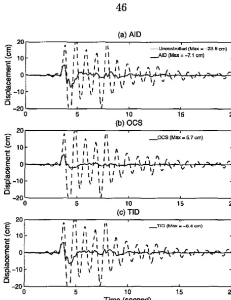
TID Algorithms Excited by the SCH Ground Motion, Type 1 Configuration 46
2.29 Velocity Time Histories of the PS Controlled by the AID, OCS, and TID
Algorithms Excited by the SCH Ground Motion, Type 1 Configuration . . . 46
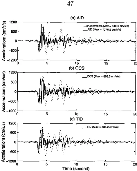
2.30 Acceleration Time Histories of the PS Controlled by the AID, OCS, and TID
2.31 Displacement Time Histories of the AS Controlled by the AID, OCS, and
TID Algorithms Excited by the SCH Ground Motion, Type 1 Configuration 47
2.32 Acceleration Time Histories of the AS in the AID, OCS, and TID Systems
Excited by the SCH Ground Motion, Type 1 Configuration . . . 48
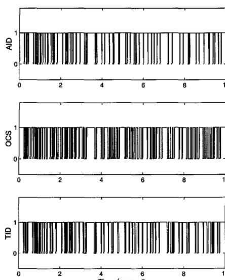
2.33 Attachment Time Histories of the AID, OCS, and TID Systems Excited by
the SCH Ground Motion, Type 1 Configuration . . . 48
2.34 Hysteresis Diagram (Control Force vs. PS Displacement) of the AID, OCS,
and TID Systems Excited by the SCH Ground Motion, Type 1 Configuration 49
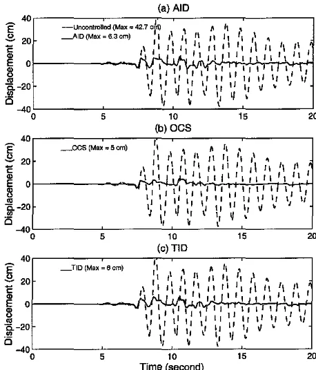
2.35 Displacement Time Histories of the PS Controlled by the AID, OCS, and
TID Algorithms Excited by the KOB Ground Motion, Type 1 Configuration 49
2.36 Velocity Time Histories of the PS Controlled by the AID, OCS, and TID
Algorithms Excited by the KOB Ground Motion, Type 1 Configuration . . 50
2.37 Acceleration Time Histories of the PS Controlled by the AID, OCS, and TID
Algorithms Excited by the KOB Ground Motion, Type 1 Configuration . . 50
2.38 Displacement Time Histories of the AS Controlled by the AID, OCS, and
TID Algorithms Excited by the KOB Ground Motion, Type 1 Configuration 51
2.39 Acceleration Time Histories of the AS in the AID, OCS, and TID Systems
Excited by the KOB Ground Motion, Type 1 Configuration . . . 51
2.40 Attachment Time Histories of the AID, OCS, and TID Systems Excited by
the KOB Ground Motion, Type 1 Configuration . . . 52
2.41 Hysteresis Diagram (Control Force vs. PS Displacement) of the AID, OCS,
and TID Systems Excited by the KOB Ground Motion, Type 1 Configuration 52
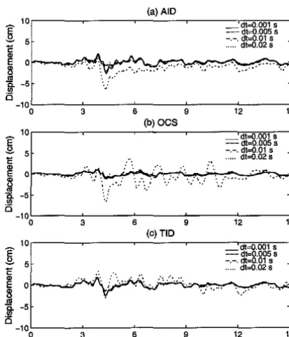
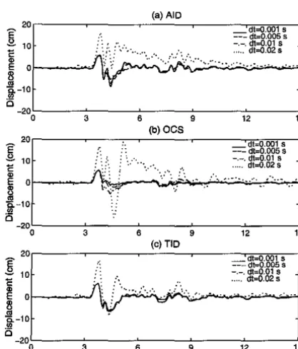
2.42 Effect of Control-Sampling Period - Displacement Time Histories of the PS
Controlled by the AIC Algorithms Under the ELC Ground Motion, Type 1
Configuration . . . 53
2.43 Effect of Control-Sampling Period - Displacement Time Histories of the PS
Controlled by the AIC Algorithms Under the HAC Ground Motion, Type 1
Configuration . . . 53
2.44 Effect of Control-Sampling Period - Displacement Time Histories of the PS
Controlled by the AIC Algorithms Under the SCH Ground Motion, Type 1
2.45 Effect of Control-Sampling Period - Displacement Time Histories of the PS
Controlled by the AIC Algorithms Under the KOB Ground Motion, Type 1
Configuration . . . 54
2.46 Effect of Control-Sampling Period - Response Spectra of the PS Controlled
by the AIC Algorithms Under the ELC Ground Motion, Type 1 Configuration 55
2.47 Effect of Control-Sampling Period - Response Spectra of the PS Controlled
by the AIC Algorithms Under the HAC Ground Motion, Type 1 Configuration 55
2.48 Effect of Control-Sampling Period - Response Spectra of the PS Controlled
by the AIC Algorithms Under the SCH Ground Motion, Type 1 Configuration 56
2.49 Effect of Control-Sampling Period - Response Spectra of the PS Controlled
by the AIC Algorithms Under the KOB Ground Motion, Type 1 Configuration 56
2.50 Effect of Time Delay - Displacement Time Histories of the PS Controlled by
the AIC Algorithms Under the ELC Ground Motion (TD
=
Time Delay),Type 1 Configuration . . . 57
2.51 Effect of Time Delay - Displacement Time Histories of the PS Controlled by
the AIC Algorithms Under the HAC Ground Motion (TD
=
Time Delay),Type 1 Configuration . . . 57
2.52 Effect of Time Delay - Displacement Time Histories of the PS Controlled by
the AIC Algorithms Under the SCH Ground Motion (TD
=
Time Delay),Type 1 Configuration . . . 58
2.53 Effect of Time Delay - Displacement Time Histories of the PS Controlled by
the AIC Algorithms Under the KOB Ground Motion (TD
=
Time Delay),Type 1 Configuration . . . 58
2.54 Effect of Time Delay - Response Spectra of the PS Controlled by the AIC
Algorithms Under the ELC Ground Motion (TD
=
Time Delay), Type 1Configuration . . . 59
2.55 Effect of Time Delay - Response Spectra of the PS Controlled by the AIC
Algorithms Under the HAC Ground Motion (TD
=
Time Delay), Type 1Configuration . . . 59
2.56 Effect of Time Delay - Response Spectra of the PS Controlled by the AIC
Algorithms Under the SCH Ground Motion (TD
=
Time Delay), Type l2.57 Effect of Time Delay - Response Spectra of the PS Controlled by the AIC
Algorithms Under the KOB Ground Motion (TD
=
Time Delay), Type 1Configuration . . . .
3.1 Schematic of a MDOF AIC System Model .
60
90
3.2 Location and Positive Directions of Control Forces u;(t) and u2,;(t) 91
3.3 Free Body Diagrams of Lumped Mass Nodes in a MDOF Structure . 91
3.4 Outline of the Three-story Control Building: (a) Typical Floor Plan; (b)
Transverse Section; (c) Control System Layout; (d) Variable Stiffness Device
(VSD) (reprinted from reference [24]) . . . 92
3.5 Analytical Model of the Three-story Building Model 93
3.6 Outline of the Nine-story Control Benchmark Building Model (reprinted from
Ref. [29]) . . . 93
3. 7 Outline of the 20-story Control Benchmark Building Model (reprinted from
Ref. [29]) . . . 94
3.8 Schematics of the Arrangement of the AS in the Building Models . . . 94
3.9 First Story Drift Time Histories of the Three-story Building Controlled by
the AID, OCS and TID Algorithms Respectively, Under the HAC Ground
Motion, Modal Control . . . 95
3.10 Roof Level Absolute Acceleration Time Histories of the Three-story Building
Controlled by the AID, OCS and TID Algorithms Respectively, Under the
HAC Ground Motion, Modal Control . . . 95
3.11 Distribution of (a) Maximum Interstory Drift Ratio, (b) Maximum Absolute
Acceleration in the Three-story Building Under the HAC Ground Motion,
Modal Control (-o- uncontrolled with IE always unlocked, · · · uncontrolled
with IE always locked, - - - AID, - · - · OCS, -•- TID, -!:;,,-Hysteresis Damper,
thick - 253 Damping) . . . 96
3.12 Distribution of (a) Number of Attachment, (b) Control Force, (c) AS
Dis-placement Relative to the Support Floor, (d) AS Absolute Acceleration in
the Three-story Building Under the HAC Ground Motion, Modal Control
3.13 First Story Drift Time Histories of the Three-story Building Controlled by
the AID, OCS and TID Algorithms Respectively, Under the KOB Ground
Motion, Modal Control . . . 97
3.14 Roof Level Absolute Acceleration Time Histories of the Three-story Building
Controlled by the AID, OCS and TID Algorithms Respectively, Under the
KOB Ground Motion, Modal Control . . . 97
3.15 Distribution of (a) Maximum Interstory Drift Ratio, (b) Maximum Absolute
Acceleration in the Three-story Building Under the KOB Ground Motion,
Modal Control (-o- uncontrolled with IE always unlocked, · · · uncontrolled
with IE always locked, - - - AID, - · - · OCS, -•- TID,
-L-
Hysteresis Damper,thick - 25% Damping) . . . 98
3.16 Distribution of (a) Number of Attachment, (b) Control Force, (c) AS
Dis-placement Relative to the Support Floor, (d) AS Absolute Acceleration in
the Three-story Building Under the KOB Ground Motion, Modal Control
(-- (-- AID, (-- · (-- · OCS, (-- TID, thick - 25% Damping) . . . 98
3.17 First Story Drift Time Histories of the Nine-story Building Controlled by
the AID, OCS and TID Algorithms Respectively, Under the ELC Ground
Motion, Modal Control . . . 99
3.18 Roof Level Absolute Acceleration Time Histories of the Nine-story Building
Controlled by the AID, OCS and TID Algorithms Respectively, Under the
ELC Ground Motion, Modal Control . . . 99
3.19 Distribution of (a) Maximum Interstory Drift Ratio, (b) Maximum Absolute
Acceleration in the Nine-story Building Under the ELC Ground Motion,
Modal Control (-o- uncontrolled with IE always unlocked, · · · uncontrolled
with IE always locked, - - - AID, - · - · OCS, _,_ TID, -L- Hysteresis Damper,
thick - 25% Damping) . . . 100
3.20 Distribution of (a) Number of Attachment, (b) Control Force, (c) AS
Dis-placement Relative to the Support Floor, (d) AS Absolute Acceleration in
the Ninestory Building Under the ELC Ground Motion, Modal Control (
3.21 First Story Drift Time Histories of the Nine-story Building Controlled by
the AID, OCS and TID Algorithms Respectively, Under the SCH Ground
Motion, Modal Control . . . 101
3.22 Roof Level Absolute Acceleration Time Histories of the Nine-story Building
Controlled by the AID, OCS and TID Algorithms Respectively, Under the
SCH Ground Motion, Modal Control . . . 101
3.23 Distribution of (a) Maximum Interstory Drift Ratio, (b) Maximum Absolute
Acceleration in the Nine-story Building Under the SCH Ground Motion,
Modal Control (-o- uncontrolled with IE always unlocked, · · · uncontrolled
with IE always locked, - - - AID, - · - · OCS, -•- TID, -6- Hysteresis Damper,
thick - 253 Damping) . . . 102
3.24 Distribution of (a) Number of Attachment, (b) Control Force, (c) AS
Dis-placement Relative to the Support Floor, (d) AS Absolute Acceleration in
the Ninestory Building Under the SCH Ground Motion, Modal Control (
-- AID, -- · -- · OCS, -- TID, thick - 253 Damping) . . . 102
3.25 First Story Drift Time Histories of the 20-story Building Controlled by the
AID, OCS and TID Algorithms Respectively, Under the ELC Ground
Mo-tion, Modal Control . . . 103
3.26 Roof Level Absolute Acceleration Time Histories of the 20-story Building
Controlled by the AID, OCS and TID Algorithms Respectively, Under the
ELC Ground Motion, Modal Control . . . 103
3.27 Distribution of (a) Maximum Interstory Drift Ratio, (b) Maximum Absolute
Acceleration in the 20-story Building Under the ELC Ground Motion, Modal
Control (-o- uncontrolled with IE always unlocked, · · · uncontrolled with IE
always locked, - - - AID, - · - · OCS, -•- TID, -6- Hysteresis Damper, thick
- 253 Damping) . . . 104
3.28 Distribution of (a) Number of Attachment, (b) Control Force, (c) AS
Dis-placement Relative to the Support Floor, (d) AS Absolute Acceleration in
the 20story Building Under the ELC Ground Motion, Modal Control (
3.29 First Story Drift Time Histories of the 20-story Building Controlled by the
AID, OCS and TID Algorithms Respectively, Under the SCH Ground
Mo-tion, Modal Control . . . 105
3.30 Roof Level Absolute Acceleration Time Histories of the 20-story Building
Controlled by the AID, OCS and TID Algorithms Respectively, Under the
SCH Ground Motion, Modal Control . . . 105
3.31 Distribution of (a) Maximum Interstory Drift Ratio, (b) Maximum Absolute
Acceleration in the 20-story Building Under the SCH Ground Motion, Modal
Control (-o- uncontrolled with IE always unlocked, · · · uncontrolled with IE
always locked, - - - AID, - · - · OCS, -•- TID, -6- Hysteresis Damper, thick
- 25% Damping) . . . 106
3.32 Distribution of (a) Number of Attachment, (b) Control Force, (c) AS
Dis-placement Relative to the Support Floor, (d) AS Absolute Acceleration in
the 20story Building Under the SCH Ground Motion, Modal Control (
-AID, - · - · OCS, - TID, thick - 25% Damping) 106
3.33 First Story Drift Time Histories of the Three-story Building Controlled by
the AID, OCS and TID Algorithms Respectively, Under the HAC Ground
Motion, Nodal Control . . . 107
3.34 Roof Level Absolute Acceleration Time Histories of the Three-story Building
Controlled by the AID, OCS and TID Algorithms Respectively, Under the
RAC Ground Motion, Nodal Control . . . 107
3.35 Distribution of (a) Maximum Interstory Drift Ratio, (b) Maximum Absolute
Acceleration in the Three-story Building Under the HAC Ground Motion,
Nodal Control (-o- uncontrolled with IE always unlocked, . · · uncontrolled
with IE always locked, - - - AID, - · - · OCS, -•- TID, -6- Hysteresis Damper) 108
3.36 Distribution of (a) Number of Attachment, (b) Control Force, (c) AS
Dis-placement Relative to the Support Floor, (d) AS Absolute Acceleration in
the Three-story Building Under the RAC Ground Motion, Nodal Control
(-- (-- AID, (-- · (-- · OCS, (-- TID) . . . 108
3.37 First Story Drift Time Histories of the Nine-story Building Controlled by
the AID, OCS and TID Algorithms Respectively, Under the ELC Ground
3.38 Roof Level Absolute Acceleration Time Histories of the Nine-story Building
Controlled by the AID, OCS and TID Algorithms Respectively, Under the
ELC Ground Motion, Nodal Control . . . 109
3.39 Distribution of (a) Maximum Interstory Drift Ratio, (b) Maximum Absolute
Acceleration in the Nine-story Building Under the ELC Ground Motion,
Nodal Control (-o- uncontrolled with IE always unlocked, · · . uncontrolled
with IE always locked, - - - AID, - · - · OCS, -*- TID, -6- Hysteresis Damper) 110
3.40 Distribution of (a) Number of Attachment, (b) Control Force, (c) AS
Dis-placement Relative to the Support Floor, (d) AS Absolute Acceleration in
the Ninestory Building Under the ELC Ground Motion, Nodal Control (
-- AID, -- · -- · OCS, -- TID) . . . 110
3.41 First Story Drift Time Histories of the 20-story Building Controlled by the
AID, OCS and TID Algorithms Respectively, Under the ELC Ground
Mo-tion, Nodal Control . . . 111
3.42 Roof Level Absolute Acceleration Time Histories of the 20-story Building
Controlled by the AID, OCS and TID Algorithms Respectively, Under the
ELC Ground Motion, Nodal Control . . . 111
3.43 Distribution of (a) Maximum Interstory Drift Ratio, (b) Maximum Absolute
Acceleration in the 20-story Building Under the ELC Ground Motion, Nodal
Control (-o-uncontrolled with IE always unlocked, · · · uncontrolled with IE
always locked, - - - AID, - · - · OCS,
-*-
TID) . . . 1123.44 Distribution of (a) Number of Attachment, (b) Control Force, (c) AS
Dis-placement Relative to the Support Floor, (d) AS Absolute Acceleration in
the 20story Building Under the ELC Ground Motion, Nodal Control (
-AID, - · - · OCS, - TID) . . . 112
4.1 General Appearance of Power Spectral Density Function S(w) 136
4.2 A Typical Gaussian Process and Its Power Spectral Density Function S(w) 136
4.3 Intensity Envelope Function e(t) for Nonstationary Process a(t) 137
4.4 A Typical Artificial Ground Motion Accelerogram . . . 137
4.5 Normalized Occurrence Frequency of the Maximum Displacement of PS (a=
4.6 Normalized Occurrence Frequency of the Maximum Absolute Acceleration of
PS (a = 2, If; = 10, 17 = 0.6) . . . 138
4.7 Normalized Occurrence Frequency of the Attachment Number (a= 2, If; =
10, '7 = 0.6) . . . 139
4.8 Variation of Mean Values of (a) Maximum Displacement of PS; (b)
Maxi-mum Absolute Acceleration of PS; (c) Average Control Force; (d)
Attach-ment Number; (e) Number of Peak DisplaceAttach-ments of PS; (f) Number of Peak
Absolute Acceleration of PS; (g) Maximum Displacement of AS; (h)
Maxi-mum Absolute Acceleration of AS with Stiffness Ratio a ( l/;=10, o AID with
(2=23, lo. AID with (2=153, x OCS with (2=23,
+
OCS with (2=153) . 1394.9 Variation of Mean Values of (a) Maximum Displacement of PS; (b)
Maxi-mum Absolute Acceleration of PS; (c) Average Control Force; (d) Attachment
Number; (e) Number of Peak Displacements of PS; (f) Number of Peak
Ab-solute Acceleration of PS; (g) Maximum Displacement of AS; (h) Maximum
Absolute Acceleration with Frequency Ratio If; ( a=2, o AID with ( 2=23,
to.
AID with (2=153, x OCS with (2=23,
+
OCS with (2=153) . . . 1404.10 Variation of Mean Values of (a) Maximum Displacement of PS; (b)
Maxi-mum Absolute Acceleration of PS; (c) Average Control Force; (d) Attachment
Number; (e) Number of Peak Displacements of PS; (f) Number of Peak
Ab-solute Acceleration of PS; (g) Maximum Displacement of AS; (h) Maximum
Absolute Acceleration of AS with AS Damping Ratio (2 (a=2, l/;=10, o AID,
x OCS) . . . 140
4.11 Variation of Mean Values of (a) Maximum Displacement of PS; (b)
Maxi-mum Absolute Acceleration of PS; ( c) Average Control Force; ( d) Attachment
Number; (e) Number of Peak Displacements of PS; (f) Number of Peak
Ab-solute Acceleration of PS; (g) Maximum Displacement of AS; (h) Maximum
Absolute Acceleration of AS with Control Force Limit Ratio 17 ( a=2, l/;=10,
o TID with (2=23, x TID with (2=153) . . . 141
B.l A SDOF AIC Model . . . 153
B.2 Configuration of the AIC System at
t
= 0 154B.4 Configuration of the AIC System at
t
= t2 (a< 1)B.5 Configuration of the AIC System at
t
= t2 (a> 1)B.6 Configuration of the AIC System at
t
= t3 (a< 1)B.7 Configuration of the AIC System at
t
= t3 (a> 1)B.8 Configuration of the AIC System at t=O .
B.9 Configuration of the AIC System at
t
= tiB.10 Configuration of the AIC System at t = t2 (a< 1)
B.11 Configuration of the AIC System at
t
= t2 (a> 1)B.12 Configuration of the AIC System at
t
= t3 (a< 1)B.13 Configuration of the AIC System at t = t3 (a> 1)
B.14 Configuration of the AIC System at
t
= 0B.15 Configuration of the AIC System at
t
=tiB.16 Configuration of the AIC System at
t
= t2 (w9/w3<
1) . B.17 Configuration of the AIC Systemt
= t2 (w9/w3>
1) B.18 Configuration of the AIC System att
= 0 .B.19 Configuration of the AIC System at
t
=ti .157
159
160
161
161
163
165
167
169
169
170
171
173
173
176
List of Tables
2.1 Characteristics of the AIC Control Algorithms . . . 15
2.2 Variations of Equivalent Damping Ratio ( for the AID and OCS System 19
2.3 Maximum Value of the PS Acceleration, Velocity, and Displacement
Re-sponse Under Harmonica! Excitation, Type 1 Configuration . . . 23
2.4 Acceleration, Velocity, and Displacement of the PS and AS Under ELC
Ground Motion
2.5 Acceleration, Velocity, and Displacement of the PS and AS Under HAC
Ground Motion
2.6 Acceleration, Velocity, and Displacement of the PS and AS Under SCH
Ground Motion
2.7 Acceleration, Velocity, and Displacement of the PS and AS Under KOB
Ground Motion
2.8 Number of Attachments Between the PS and AS in the Entire 30-second
Duration of Input Ground Motion ELC, HAC, SCH, and KOB for the AID,
OCS and TID Algorithms . . . .
3.1 Characteristics of the AIC Control Algorithms (Modal Control)
3.2 Characteristics of the AIC Control Algorithms (Nodal Control)
3.3 Characteristics of the Auxiliary Structures in the Three-story Building .
3.4 Characteristics of the Auxiliary Structures in the Nine-story Building
3.5 Characteristics of the Auxiliary Structures in the 20-story Building .
3.6 Response of the Three-story Building, Modal Control .
3.7 Response of the Three-story Building, Nodal Control .
3.8 Response of the Nine-story Building, Modal Control
3.9 Response of the Nine-story Building, Nodal Control
3.10 Response of the 20-story Building, Modal Control .
3.11 Response of the 20-story Building, Nodal Control .
4.1 Parameters of the UBC Design Spectrum [40] . . .
26
27
27
28
29
71
72
75
76
79
83
84
86
87
87
89
4.2 Statistics of the Uncontrolled Response From the Simulation Results (Unit:
m, sec) . . . 123
4.3 Statistics of the AID-Controlled Response With Varying Stiffness Ratio a
((2 = 2%, 'ljJ = 10) From the Simulation Results (Unit: m, sec) . . . 124
4.4 Statistics of the OCS-Controlled Response With Varying Stiffness Ratio a
((2
=
2%, 'ljJ=
10) From the Simulation Results (Unit: m, sec) . . . 1254.5 Statistics of the AID-Controlled Response With Varying Stiffness Ratio a
((2
=
15%, 'ljJ=
10) From the Simulation Results (Unit: m, sec) 1264.6 Statistics of the OCS-Controlled Response With Varying Stiffness Ratio a
((2 = 15%, 'ljJ = 10) From the Simulation Results (Unit: m, sec) 127
4. 7 Statistics of the AID-Controlled Response With Varying Frequency Ratio 'ljJ
((2 = 2%, a = 2) From the Simulation Results (Unit: m, sec) . . . 128
4.8 Statistics of the OCS-Controlled Response With Varying Frequency Ratio 'ljJ
((2
=
2%, a= 2) From the Simulation Results (Unit: m, sec) . . . 1294.9 Statistics of the AID-Controlled Response With Varying Frequency Ratio 'ljJ
((2
=
15%, a= 2) From the Simulation Results (Unit: m, sec) . . . 1304.10 Statistics of the OCS-Controlled Response With Varying Frequency Ratio 'ljJ
((2
= 15%, a
= 2) From the Simulation Results (Unit: m, sec) . . . 131
4.11 Statistics of the AID-Controlled Response With Varying AS Damping Ratio
( 2 (a= 2, 'ljJ = 10) From the Simulation Results (Unit: m, sec) . . . 132
4.12 Statistics of the OCS-Controlled Response With Varying AS Damping Ratio
( 2 (a= 2, 'ljJ = 10) From the Simulation Results (Unit: m, sec) . . . 133
4.13 Statistics of the TID-Controlled Response With Varying Control Force Limit
ratio '1 (a= 2, 'ljJ = 10, (2 = 2%) From the Simulation Results (Unit: m, sec) 134
4.14 Statistics of the TID-Controlled Response With Varying Control Force Limit
ratio 17 (a= 2, 'ljJ = 10, (2 = 15%) From the Simulation Results (Unit: m, sec)135
B.1 Values of xi (t1) and x2(t1) varying with a . 156
B.2 Values of T2 Varying with a . . . 157
B.3 Values of T3 Varying with a (a:,; 1) 160
B.4 Values of T 3 Varying with a (a
>
1) 161B.6 Values of X1 (t1) and x2(t1) Varying with a and (2
B. 7 Values of r2 Varying with a and (2
B.8 Values of r3 Varying with a and (2
B.9 Values of x1 (t1) and x2(t1) Varying with a and w9
B.10 Values of r2 Varying with a and w9 • • • • • • • • •
B.11 Values of x1 (t1) and x2(t1) Varying with a and w9
B.12 Values of x1(t1) and x2(ti) Varying with a, w9 and (2
B.13 Values of r2 Varying with a, w9 and (2 . . . .
B.14 Values of x1 (t1) and x2(t1) Varying with a, w9 and (2
164
166
169
172
173
175
178
179
Nomenclature
a Stiffness Ratio between AS and PS
fJ Mass Ratio between AS and PS
1/; Frequency Ratio between AS and PS
'Y Fractional Damping Ratio between AS and PS
x9 Earthquake Ground Motion Acceleration
AIC Active Interaction Control
AID Active Interface Damping
AS Auxiliary Structure
AVD Active Variable Damping
AVS Active Variable Stiffness
DOF Degree-of-Freedom
ELC El Centro Record from the 1940 Imperial Valley Earthquake
HAC Hachinohe Record from the 1968 Tokachi-oki Earthquake
IE Interaction Element
KOB Kobe Record from the 1995 Hyogo-ken Nanbu Earthquake
MC Modal Control
MDOF: Multi-Degree-of-Freedom
NC Nodal Control
OCS Optimal Connection Strategy
PS Primary Structure
SCH Sylmar County Hospital Record from the 1994 Northridge Earthquake
SDOF : Single-Degree-of-Freedom
TID Tuned Interaction Damping
VDU Variable Damping Unit
Chapter 1 Introduction
1.1 Background and Motivation
In recent years, considerable attention has been given to research and development of
struc-tural control techniques. Successful application of strucstruc-tural control techniques will not
only greatly improve the comfort of residents in a building, but more importantly, enhance
the safety and prevent property loss when large earthquakes occur. For example, recent
destructive seismic events in Northridge, California, in 1994 and Kobe, Japan, in 1995
have demonstrated the effectiveness of mitigating these hazards by use of structural control
techniques [9].
Since the early conceptual study of structural control by Yao [45] in 1972, remarkable
progress has been made in this field. To date, numerous methods of structural control have
been proposed and some have even been implemented successfully in full-scale structures
[9, 35, 36, 3].
Consideration of energy will illustrate the working mechanisms of structural control
techniques [39, 34]. In conventionally designed structures, the vibrational energy of the
structure induced by earthquake ground motion or wind loading is dissipated through
lin-ear viscous-like damping mechanisms in the structure. However, the linlin-ear viscous-like
damping of many structures in the elastic range is insufficient to dissipate the large amount
of energy associated with strong seismic excitation. Therefore, in a major earthquake event,
a large portion of the seismic input energy must be dissipated through associated
hystere-sis by cracking and inelastic deformation of structural components. Hence damage to the
structural elements and architectural components is likely to occur. Because of economic
loss and life safety concerns, this mechanism for energy dissipation is undesirable. With the
advent of innovative concepts of structural control, it is possible to dissipate much of the
vibrational energy through external damping provided by control actions.
oscillator which has its equation of motion expressed as follows.
mx
+
ex+
kx = -mxg (1.1)By multiplying Eqn. (1.1) by
x
and integrating, the equation is transformed into an energyequation as follows.
J
mxxdt+
J
cx
2dt+
J
kxxdt =J
(-mxg)xdt'---v---' .._.,_..., ..._._,
EK En Es E1
(1.2)
where EK, En, and Es are the relative kinetic energy of the mass, the energy dissipation from linear viscous damping in the structure, and the elastic strain energy, respectively.
The sum of these energies must equal the input energy Er due to external disturbance.
For conventionally designed structures subjected to strong ground motion, it is difficult
to maintain the energy balance between the input Er and the elastic capacity of the structure
EK, En, Es. Generally, some structural components will yield or crack and the linear spring force in Eqn. (1.1) will be replaced by a nonlinear term f(x, x) typically involving hysteretic
damping effects which increase the energy dissipation capacity of the structure.
For controlled structures, a control force term u is introduced into Eqn. ( 1.1). The
energy dissipated by this control force may then be written as
Eu=
I
uxdt (1.3)The amount of hysteretic energy dissipated by yielding or cracking of the structure can be
reduced by providing the additional energy dissipation mechanism, Eu. Typically, structural
control devices are installed in places where workers have access for regular inspection
and replacement of damaged devices. Therefore, vibrational control by robust and stable
structural control approaches is obviously more attractive than the conventional means.
The control of structural vibrations produced by external loadings can be accomplished
by various means such as modifying stiffness, mass, damping, or configuration, and by
providing passive or active control forces. In general, structural control methods can be
classified into the following four categories [9]:
actuators that apply forces to the structure in a prescribed manner. These forces can
be used to both add and dissipate energy in the structure. In an active feedback
control system, the signals sent to the control actuators are a function of the response
of the system measured with physical sensors.
Passive Control A passive control system does not require an external power source.
Passive control devices impart forces that are developed in response to the motion of
the structure.
Hybrid Control A hybrid control system is typically defined as one which employs a
combined use of active and passive devices. For example, a structure equipped with
distributed viscoelastic damping supplemented by an active mass damper on or near
the top of the structure, or a base-isolated structure with actuators actively controlled
to enhance its performance.
Semi-active Control Semi-active control systems are a class of active control systems for
which the external energy requirements are orders of magnitudes smaller than typical
active control systems. Typically, semi-active control devices do not add mechanical
energy to the structural system, therefore bounded-input bounded-output stability
is guaranteed. Semi-active control devices are often viewed as controllable passive
devices.
Besides the ability of reducing selected maximum response quantities, simplicity,
re-liability, and minimal power requirement are also highly desirable for structural control
approaches. Semi-active control systems appear to combine the best features of both
pas-sive and active control systems and to offer the greatest likelihood for near-term acceptance
of control technology as a viable means of protecting civil structures against earthquake and
wind loading [35}. A semi-active control system can produce a large control force simply
by actively changing parameters such as control device damping coefficient and stiffness.
Therefore, it has the advantage that it can control the response of a large-scale structure
in a large earthquake with smaller energy in comparison with a conventional active control
system utilizing an actuator.
Recently, researchers at Kajima Corporation in Japan have conducted considerable
(5, 25, 26] and Active Variable Stiffness System (22, 23, 24, 43]. The Active Variable
Damp-ing system is a seismic response control system that uses a variable dampDamp-ing unit (VDU)
to control the damping force. The variable damping unit, which consists of a variable
hy-draulic damper and a damping force controller, can control a large damping force, although
it consumes only a small amount of electric power (25]. Both a shaking table test performed
on a three-story steel-framed structure with a mini-scale VDU (maximum force is 2 tf) and
a simulation analysis of a semi-actively controlled high-rise building confirmed the
effec-tiveness of the AVD approach in large earthquakes. Subsequently, semi-active hydraulic
dampers (SHD) which can produce a maximum damping force of 1000 kN with an electric
power of 70 watts were applied to a five-story office building located in Shizuoka City, Japan
(26). The hydraulic dampers are compact so that a large number of them can be installed
in a single building. It is thus possible to control the building's response during a large
earthquake, since a large control force is obtained in comparison with a conventional active
control system.
The Active Variable Stiffness seismic response control system has been developed to
preserve the safety of the building and important equipment contained therein against
earthquakes of large intensities (24]. The AVS system has been implemented in an actual
three-story building (KaTRl No. 21 Building) in Japan, as shown in Fig. 1.1. With this
system, the building reduces its response by establishing non-resonance against earthquake
motions. The non-resonant state is realized by altering the structure's stiffness with a
mechanical system. The AVS system can be driven by only a small amount of power.
Since the completion of the building, it has experienced three earthquakes and the observed
response confirms the effectiveness of the AVS system.
In a recent joint study with Kajima Corporation, researchers at the California Institute
of Technology have carried out a series of exploratory investigations on an innovative
struc-tural control approach, referred to as Active Interaction Control (AIC) (6, 7, 14, 41]. AIC
is developed as a semi-active means of suppressing the vibrations of structures subjected
to seismic excitation. It incorporates some important features of the AVS control approach
(7]. A typical AIC system is comprised of a primary structure targeted for control, a
num-ber of auxiliary structures and interaction elements that connect the auxiliary structures
to the primary structure. Through actively modulating the operating states of the
Figure 1.1: A Building with AVS Control Device
strategy are reactively developed within the interaction elements and the vibration of the
primary structure is thus restrained. Minimal external power is required for the operation
of interaction elements even during large earthquakes.
The first generation of AIC ~ the Active Interface Damping (AID) control algorithm was
developed by Hayen and Iwan [6, 8]. This control approach utilizes controlled interactions
between two distinct structural systems, or different components of the same structure to
suppress the resonance buildup that develops in the primary structure during an external
excitation. The AID control algorithm is implemented by minimizing the rate of change
in the vibrational energy of the primary structure for each control-sampling period. Linear
single- and multi-degree-of-freedom models have been considered to examine the
perfor-mance of the AID algorithm.
The next generation of AIC, Optimal Connection Strategy (OCS), was developed by
Wang and Iwan [14, 41]. Their OCS control algorithm is based on a set of three simultaneous
conditions for an attachment between the primary structure and auxiliary structure. If at
some representative time point, all of the three conditions are satisfied, a "Locked" state will
be applied to the interaction element in the next control-sampling period and interaction
between the primary structure and auxiliary structure are thus activated. An "Unlocked"
state is applied to the interaction element if any of these three conditions is not met. Because
of the rule-based nature of this control algorithm, it is rather difficult to implement this
Although the OCS control algorithm generally exhibits better control performance than
the AID control algorithm when time delays are ignored, the excessively large number
of interaction cycles associated with this algorithm presents a problem. If the duration
of the "Locked" state is too short, the interaction element may not react fast enough to
produce the desired effect due to its mechanical limitations. Large accelerations are also
observed in the OCS-controlled primary structure. These problems partially motivate the
investigation described in this thesis. Another incentive for this study is to test the AIC
control algorithms within the framework of more realistic structural models.
1.2
Scope and Organization of the Thesis
This thesis summarizes the result of a follow-on study on the AIC control algorithm. The
mechanism associated with the over-attachment problem in the original OCS system is
clar-ified and corresponding counter-measures are proposed. The OCS algorithm is reformulated
within an energy framework and therefore all of the AIC control algorithms are unified
un-der the same instantaneous optimal control strategy. The effectiveness of the AIC control
algorithms is verified through numerical simulation results for 3-story, 9-story and 20-story
steel-framed buildings. The statistical behavior of the AIC system is evaluated based on a
Monte Carlo simulation.
In Chapter 2, the working mechanism and associated control strategy underlying the
AIC control algorithms are illustrated using a single-degree-of-freedom (SDOF) structure
model. Founded upon the same instantaneous optimal control strategy, three sub-AIC
algorithms, namely, the Active Interface Damping (AID), Optimal Connection Strategy
(OCS) and newly developed Tuned Interaction Damping (TID) algorithms are discussed.
A typical SDOF AIC system consists of a primary structure, an auxiliary structure and
an interaction element linking the primary structure and auxiliary structure together. To
simplify the subsequent analysis, assumptions are made regarding the primary structure
and auxiliary structure at the beginning of this chapter. Two models are considered for
the interaction element. The stability of an unforced AIC system is shown using the
Lya-punov direct method. The effectiveness of AIC control algorithms is then demonstrated
by numerical simulations of SDOF AIC systems subjected to various types of excitation.
effectiveness in an actual implementation of the AIC approach are considered. Specifically,
the following two constraints are addressed for the AIC systems: control-sampling period
and presence of time delays.
Eventually, any structural control approach needs to be implemented in more realistic
multi-degree-of-freedom (MDOF) structural models. In Chapter 3, the AIC algorithm is
reformulated within the framework of linear MDOF systems. Two approaches, the Modal
Control and Nodal Control approaches, are developed to implement the AIC control
algo-rithms in MDOF systems. The Modal Control approach directs the control effort to certain
dominant response modes of the primary structure, while the Nodal Control approach tries
to restrain the individual inter-story drift of the structure directly. Three structures, a
3-story building, a 9- and a 20-3-story steel-framed building controlled with the AIC algorithms
are analyzed for several historical earthquake records.
Chapter 4 describes the statistical behavior of SDOF AIC systems. A large ensemble
of artificial earthquake ground motions is generated from modified Kanai-Tajimi filtered
gaussian white-noise process. Using this ensemble of artificial earthquake ground motions,
a Monte Carlo simulation is carried out to assess the performance of SDOF AIC systems
in a statistical sense. The parameters which have significant effects on the performance of
AIC systems are the stif!lless ratio a, frequency ratio 'lj;, AS damping ratio (z and control
force limit Umax. The optimal values of these important parameters are determined based
on the same ensemble of artificial seismic ground motions.
Chapter 5 contains the main conclusions of the work presented in this thesis and some
Chapter 2 Active Interaction Control of Linear
SDOF Systems
2.1
Introduction
The AIC control approach has been proposed as a semi-active means of protecting structures
against large earthquakes. In this chapter, a simple Active Interaction Control (AIC) system
model involving two interacting SDOF systems is investigated. One of the SDOF systems is
the primary structure targeted for vibration control while the other is the auxiliary structure
for delivering the control force needed. Although this is a highly idealized model of complex
building systems, it is fundamental to the understanding of the essential dynamic behavior
of more complicated AIC systems.
In an AIC system, an interaction element which links the primary structure and auxiliary
structure together is employed to facilitate the interactions between the primary structure
and auxiliary structure. The objective of the control strategy under investigation is to
reduce the motion of the primary structure as much as possible. Through actively controlled
interactions, control force favorable to this control strategy can be generated within the
interaction element. This control force plays the role of removing vibrational energy from
the primary structure to the auxiliary structure. When the interaction is activated, part of
the vibrational energy of the primary structure is transmitted into the auxiliary structure
where it will be dissipated in the following cycles when the interaction is deactivated.
The AIC algorithms include the Active Interface Damping (AID) [6, 7], the Optimal
Connection Strategy (OCS) [41, 14, 15], and newly developed Tuned Interaction Damping
(TID)
algorithms. All of these AIC algorithms may be founded upon the same instantaneousoptimal control strategy that involves minimization of an energy-based performance index
at every time instant. The effectiveness of AIC algorithms is demonstrated by numerical
simulations of SDOF AIC systems subjected to various types of excitations. Finally, two
practical constraints which are expected to have a significant impact on control effectiveness
following two constraints are addressed for the AIC systems: control-sampling period and
presence of time delays.
2.2
Assumptions and Formulation
For convenience and simplicity, the following acronyms are defined and will be used in the
following discussion.
PS: Primary Structure; AS: Auxiliary Structure; IE: Interaction Element
The following assumptions are made in this study:
• Only response in the horizontal direction is considered.
• All system parameters are known in advance and do not change during the excitation
duration. The PS and AS remain within the linear elastic range.
• The mass of IE is negligible compared to that of PS and AS and therefore the dynamics
of IE is neglected. It is further assumed that an IE can respond instantaneously to
control signals except for the cases with time delay.
• The system states are completely observable. Only present and past values of base
acceleration and system state variables are available to determine the control input.
Under these conditions, the equations of motion for the PS and AS subjected to base
excitation
x
9 are expressed aswhere
Mx(t)
+
C:X:(t)+
Kx(t)=
-MLx9(t)+
ru(t)x(t)
= {
x1 (t) x2(t)}T is the relative displacement vector,is the mass matrix, C
= [
ci O ]0 C2
K
= [
ki O ] is the stiffness matrix,0 k2
is the damping matrix,
and mi, m2, c1, c2, ki, k2, and x1, X2 represent the mass, stiffness, damping factor, and
relative displacement of the PS and AS respectively, as shown in Fig. 2.1. The subscripts
1 and 2 are used to denote the PS and AS respectively.
x
9 is the ground acceleration. u(t)is the control force developed within the IE; the sign of u(t) is defined such that u(t) is
positive whenever the IE is in tension.
Rewriting the above equations of motion in the state-space form yields
X(t) = AX(t)
+
Buu(t)+
Bww(t) (2.2)where
X(t) = {x(t) x(t)}T is the state vector,
A=
w(t)
=
i 9(t) represents the external excitation,and 0v, 0 and I denote the null vector, null matrix and identity matrix, respectively.
In structures, the displacements and velocities of the system masses are commonly used
as state variables. The above linear state equation is widely used in conventional optimal
control problems and will form the basis for the formulation and solution of system
dy-namics in this study. By using the state equations, the well-known second-order differential
equations characterizing the motion of a structural system can be rewritten as a set of
first-order differential equations. Current techniques for the high-speed solution of first-first-order
differential equations make the state-space approach particularly attractive.
To compute the dynamics of an AIC system subjected to external disturbance, a
nu-merical scheme in discrete time has to be employed because of the nonlinearity and history
dependence associated with the AIC system. The state variable, X(tk+I) at time tk+I for
the given initial condition X(tk) at time tk, is given by the following convolution integral:
A partitioned predictor-corrector (PPC) method [13] is employed for computing the
integral in Eqn. (2.3). A brief description of the PPC method is given in Appendix A.
Using this numerical scheme, X ( tk+l) can be expressed as
where
ii> = eAL>t
Bui = A-1[il> - A-l(J - il>)]B /::,.t u
Bu2 A-1[A-1(il> -/::,.t I) - I]B u
Bw1 A-l[il> - A-l(J - il>)]B /::,.t w
Bw2 A-1[A-1(q; -/::,.t I) - I]B w (2.5)
and u(tk+1) is the estimated value of the control force vector as described in Appendix A.
2.3 Interaction Elements
Two types of IEs are considered in this study. These are depicted in Fig. 2.2. The first
type, Type A IE, consists only of an On/ Off locking device which has two operating states:
locked or unlocked. In its locked state, a rigid connection is provided between the PS and AS, while in its unlocked state, the force developed within the IE is equal to zero and it is
further assumed that the transition from the locked state to unlocked state or the converse
is accomplished instantaneously. A Type B IE is comprised of a fuse device and an On/ Off
locking device described above which are placed in series with each other. The mechanical
properties of Type B IE is the same as that of Type A IE except that control force in a
Type A IE is not allowed to exceed a pre-specified maximum value which depends on the
property of the fuse device. Examples of the fuse device could be a Coulomb frictional
damper or a hydraulic pressure-limiting device. It is noteworthy that recently developed
magneto-rheological damper can also be used for this purpose.
The expression for the force reactively developed within the IE is given below for each
• Type A: On/Off locking device
u = m1
+
m2 m1+
m 2 1 {(m1k2x2-m2k1x1)+(m1c2-m2c1):i; ,locked
0 , unlocked
(Note that in the locked state, it is assumed that x 1 = x2, and :i;1 = ±2.)
• Type B: On/Off locking device placed in series with a fuse device
u
=
UmaxSgn(xi - ±2), lul
'.O Umax, lul
>
Umax,locked
(2.6)
{ {
( m1 kzx2 - m2k1x1) m1 + m2 + (m1c2 - m2c1 m1
+
m2 )x 10 , unlocked
(2.7)
where Umax is the control force limit associated with the fuse device and Sgn( ·) is the
signum function.
2.4 Control Strategy and Stability
Vibration control for seismically excited structures presents a unique problem since the
excitation input, the earthquake ground motion, is generally unknown a priori. Also, it is
usually unrealistic to provide the large power source necessary to apply the control force
determined from an active control law during significant seismic events. Therefore, new
optimal control strategies suitable for controlling earthquake-excited structures is highly
desired. In this section, one such type of instantaneous optimal control algorithm is
dis-cussed. This algorithm was originally developed by Hayen and Iwan [6, 8].
The aim of the AIC control strategy is to reduce the motion of the PS as much as
possible. This objective can be achieved by minimizing the time derivative of the relative
vibrational energy of the PS at each time instant during external excitations. The relative
vibrational energy of the PS is defined as
(2.8)
vibrational energy of the PS is expressed as
(2.9)
In practice, any control algorithm has to be implemented in discrete time. Consider
some time interval [to, ti] during which vibration control for the PS is to be accomplished.
Let [to, ti] be uniformly partitioned into a set of appropriately short time intervals, each of
duration At and referred to as a control-sampling period. Now, consider a representative
time interval, the kth control-sampling period, defined by
t
E[tk, tk+i)·
As noted above,ef-fort is directed toward minimizing the change in E 1 for the control-sampling period, denoted
by AEf, or causing this change to be as negative as possible.
1
tk+l[-u(t) - m1x9 - c1±1]±1dt
tk
"" -[u(t)±1]
I
At -[m1x
9
±1+c1±~]1
At+ 0(At2)t=tk t=tk (2.10)
If the sampling period is small enough, the higher order term O(At2
) can be neglected.
In addition, the second term in Eqn. (2.10) is uncontrollable in the sense that it is constant
regardless of the operating state selected for the IE. Hence, to the degree of approximation
considered, the difference in values of AE~ for different IE operating states depends solely
on the first term in Eqn. ( 2 .10) .
The control strategy can now be described as follows: at the beginning of each
control-sampling period, the state variables X(t) of the PS and AS are measured and thus fully known. A control processor then uses this information to determine an appropriate
oper-ating state for the IE: locked or unlocked. In the locked state, interactions between the
PS and AS are activated, while interactions are deactivated in the unlocked state. Finally,
the control signal made at the beginning of each control-sampling period is sent to the
control valve of the IE to switch or maintain the operating state of the IE. The system then
responds to the values of u(t) resulting from these interactions until the beginning of next
control-sampling period, when another appropriate operating state is determined for the
IE. This procedure is then repeated for each consecutive control-sampling period [6].
instan-taneous optimal control strategy with its performance index defined by
(2.11)
where
(2.12)
By minimizing
Ei,
the performance index J(t) is kept as low as possible at each timeinstant
t
E[t
0 ,ti].
Unlike the active control case in which any desired control force canbe applied, a constraint is imposed on the available control force in an AIC system
be-cause of its inherent interaction characteristics. That is, the control force u(t) in the next control-sampling period is described by Eqns. (2.6) or (2. 7). Therefore, minimization of
the performance index J(t) is done by substituting the control force value in one of the two
distinct states: locked or unlocked. If j(tk)locked is less than j(tk)unlocked at discrete time
instant tk, an interaction will be activated between the PS and AS in the next sampling
period, and vice versa. Because minimization is done only at discrete time instant and for
very limited number of (two for the the IE considered in this study) IE operating states,
the AIC algorithms are only sub-optimal
[6].
A heuristic control law for the AIC control strategy can be expressed by the
attach-ment conditions summarized in Table 2.1 for each AIC algorithm. When the attachattach-ment
conditions for a particular AIC algorithm are satisfied simultaneously at the beginning of a
control-sampling period, a locked state is selected for the IE, while the IE is unlocked if one
of the attachment conditions is not satisfied. It is seen that one condition which drives the
first term at the right-hand side of Eqn. (2.10) as negative as possible is employed by all
AIC algorithms which include the AID, OCS and TID algorithms. This condition is derived
from the above-formulated instantaneous optima] control strategy. It is also observed that
the physical meaning of this condition ensures that no mechanical energy will be put in to
the PS from the AS since ±1 (t) actually represents the energy dissipation rate of PS.
When the PS and AS are attached with dissimilar velocities, the induced impact may
cause damage to either or both the PS and AS. This detrimental impact effect can be
elim-inated if an additional attachment condition is introduced. This new attachment condition
Table 2.1: Characteristics of the AIC Control Algorithms
Control Attachment AS Dynamics IE Type and
Algorithms Conditions Operating States
AID u"(t) · ±1 (t) ;::: 0 Considered Type A, Free/Rigid
ocs
Considered Type A, Free/Rigid{
u"(t) · ±1(t)2
0 ±1 (t)=
±2(t)TID Considered TypeB,
{
u"(t) · ±1 (t)2
0 Free/Rigid/Slip,lu"(t)I :::; Umax ±1(t)
=
±2(t)Note: AIC control algorithms include the Active Interface Damping (AID), Optimal Connection Strategy {OCS), and Tuned Interaction Damping {TID) algorithms. u"(t) represents the control force value calculated from the assumption that the PS is attached to the AS at time t (i.e., the IE is assumed to be locked).
AS.
However, other important reasons exist for the adoption of this additional attachment
condition besides eliminating the impact effect. In an AIC system, the function of the AS
can be regarded as an actuator delivering a control force to the PS. The value of the control
force delivered by the AS is approximately equal to the elastic spring restoring force in the
AS. Therefore, the larger the AS displacement, the larger the control force will be. It is
found that the PS and AS usually achieve equal velocities at the time instant when the AS
is close to its maximum displacement position. A large control force will then be generated
and more energy will be dissipated from the PS if the attachment between the PS and AS
is delayed until the PS and AS have equal velocities. This study shows that doing this
not only will many interaction opportunities not be missed, but this new algorithm has an
improved response reduction capability.
Stability is an important concer