Applied Computational Topology for Point Clouds and Sparse Timeseries Data

and Sparse Timeseries Data

Thesis by

Melissa Yeung

In Partial Fulfillment of the Requirements for the degree of

Doctor of Philosophy

CALIFORNIA INSTITUTE OF TECHNOLOGY Pasadena, California

2017

c

₂₀₁₇

ACKNOWLEDGEMENTS

The opportunity to devote uninterrupted time to graduate studies is one of great privilege. A graduate education often marks the beginning of a research career, where one endeavors to expand human knowledge and to make the world a better place for the next generation. Thus, first and foremost, I would like to thank the United States taxpayer, for contributing their hard-earned dollars so that I could have the opportunity to learn, to dream, and to discover.

This dissertation would not have been possible without the support of my advisor, Mathieu Desbrun. Thank you for the freedom to explore, the op-portunity to find my own path, for letting me take the scenic route. I also owe much of my graduate experience to Dmitriy Morozov, who has been an indispensable guide and mentor in the world of computational topology and life. Thank you for teaching me the fundamentals—both in computa-tional topology and in high performance computing—and for ensuring that I would always have opportunities—opportunities to present my work, to learn computational topology from the luminaries, and to find belonging in one of the most supportive and welcoming mathematical communities. The journey that led me to a Ph.D. is improbable. I owe many of my successes along this journey to the numerous individuals who have supported and encouraged me along the way: Miklos Abert, David Beckstead, Collin Bleak, Karen Brucks, Danny Calegari, Gunnar Carlsson, Michael Dorff, Benson Farb, Erica Flapan, Deanna Haunsperger, Stephen Kennedy, David E. Keyes, Robert Maddock, J. Peter May, Konstantin Mischaikow, Paul J. Sally, Jr., Wilhelm Schlag, Stephen Skapek, Liz Stanhope, Glenn Stevens, Elizabeth Townsend, and Samuel L. Volchenboum.

ABSTRACT

The proliferation of sensors and advancement of technology has led to the production and collection of unprecedented amounts of data in recent years. The data are often noisy, non-linear, and high-dimensional, and the eff ective-ness of traditional tools may be limited. Thus, the technological advances that enable the ubiquitous collection of data from the cosmological scale to the subatomic scale also necessitate the development of complementary tools that address the new nature of the data.

Recently, there has been much interest in and success with developing topologically-motivated techniques for data analysis. These approaches are especially useful when a topological method is sensitive to large- and small-scale features that might not be detected by methods that require a level of geometric detail that is not provided by the data or by methods that may obscure geometric features, such as principal component analysis (PCA), multidimensional scaling (MDS), and cluster analysis.

Our work explores topological data analysis through two frameworks. In the first part, we provide a tool for detecting material coherence from a set of spatially sparse particle trajectories via the study of a map induced on homology by the braid corresponding to the motion of particles. While the theory of coherent structures has received a great deal of attention and benefited from many advances in recent years, many of these techniques are limited when the data are sparse. We demonstrate through various examples that our work provides a practical and scalable tool for identifying coherent sets from a sparse set of particle trajectories using eigenanalysis.

TABLE OF CONTENTS

Acknowledgements . . . iii

Abstract . . . v

Table of Contents . . . vii

List of Illustrations . . . ix

Preface . . . xi

Chapter I: Introduction . . . 1

Chapter II: Braids and Material Coherence . . . 5

2.1 Introduction . . . 5

2.2 Contributions . . . 7

2.3 Braid groups . . . 9

2.4 Application to the analysis of flows . . . 15

2.5 Examples . . . 32

2.6 Discussion and future directions . . . 38

Chapter III: Topological Data Analysis . . . 41

3.1 Introduction . . . 41

3.2 Contributions . . . 42

3.3 Simplicial complexes . . . 44

3.4 Persistent homology . . . 46

3.5 Reeb graphs and Reeb spaces . . . 48

3.6 Mapper constructions . . . 55

3.7 Abstract mapper and hierarchical abstract mapper . . . 58

3.8 Application to the analysis of geospatial sensor data . . . 73

3.9 Discussion and future directions . . . 77

Nomenclature . . . 81

LIST OF ILLUSTRATIONS

Number Page

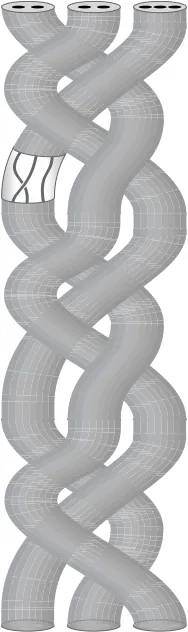
2.1 Illustration of a tubular braid . . . 8

2.2 Illustration ofσi . . . 10

2.3 Illustration ofµj . . . 19

2.4 Illustration ofσi(xi) . . . 20

2.5 Illustration ofσi(xi+1) . . . 21

2.6 Illustration of the braid corresponding toσi,η1,η2 . . . 22

2.7 Covering space action ofσi,η1,η2 . . . 23

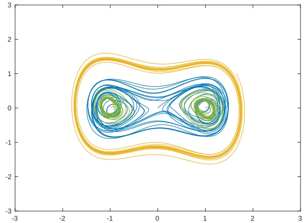
2.8 Illustrations of Poincar´e sections for Aref’s blinking vortex flow 33 2.9 Eigenvectors of the Burau matrix for Aref’s blinking vortex flow 35 2.10 Attractors of the modified Duffing oscillator . . . 36

2.11 Limit cycles of the modified Duffing oscillator . . . 37

2.12 Phase portrait of the modified Duffing oscillator . . . 37

2.13 Eigenvectors of the Burau matrix for the modified Duffing oscillator . . . 38

2.14 Two types of initial conditions for the modified Duffing oscil-lator . . . 39

3.1 Reeb graph of height function . . . 49

3.2 Step-by-step hierarchical mapper construction . . . 75

3.3 Top and cross-sectional views of the hierarchical mapper con-struction depicted in Figure 3.2 . . . 75

3.4 Mapper constructions for global sea surface temperatures. . . . 78

PREFACE

Work for this thesis is motivated by the conviction that our understanding of physical phenomena benefits greatly from a rich intersection of theory from geometry, topology, and dynamical systems. Advances in one field often inspire and bring forth paradigm shifts in another. When I began my Ph.D. studies, I was particularly interested in bringing this synchrony to computational methods for science and engineering applications. This thesis formalizes existing tools of computational topology and introduces new computational methods that allow us to detect dynamical structures from a topological lens.

Topology, since its inception, has been studied and developed as an ap-plied tool for science. Henri Poincar´e, often credited as the inventor of algebraic topology, introduced an arsenal of topological techniques and concepts through a series of papers between 1892 and 1904 about the qual-itative theory of differential equations and the long-term stability of a me-chanical system. Poincar´e’s topological ideas have been hailed as “probably the greatest advance in celestial mechanics since Newton”, as his ideas “not only breathed new life into complex analysis and mechanics; they amounted to the creation of a major new field, algebraic topology” [1].

In the 1930s, Jean Leray (with Juliusz Schauder) developed a set of alge-braic tools, including the definition and basic properties of the “topological degree” of a map (related to Brouwer’s work), to study fluid dynamics [2]. Leray’s subsequent publications throughout the rest of the 1930s provided many applications of topological principles to fluid dynamics and PDEs. ∗ In recent years, there has been a renewed interest in the interaction of geom-etry, topology, dynamics, and computation. There is a growing realization

∗

that one can devise more accurate numerical methods at no additional com-putational cost by respecting (not just approximating) the appropriate geo-metric, topological, and dynamical structures at the discrete level. Accord-ingly, researchers have developed discrete theories of geometry and topol-ogy, guided by the tenet that although continuous and discrete mathematics study different structures via different tools, many important properties and relationships can be preserved in the discrete setting under an appropriate framework. The field of discrete differential geometry was developed in this spirit by Mathieu Desbrun, Peter Schr ¨oder, and their collaborators [3, 4].

My personal interest in applied topology began with a series of conversa-tions prior to my graduate studies with Gunnar Carlsson at Stanford about his work in a field now commonly referred to as topological data analysis. In his work with coauthors, Carlsson [5] addresses the problem of identify-ing topological features in high-dimensional point clouds. In a particularly persuasive application of their algorithm, Carlsson and collaborators [6] identify a subgroup of breast cancer patients with excellent survival from microarray data. The subgroup is invisible to traditional methods of data analysis and does not fit into the accepted classification of breast cancers but has a distinct statistically significant molecular signature.

Carlsson’s success in applying topological methods of studying microarray data inspired my collaboration with Samuel Volchenboum and Stephen Skapek at the University of Chicago, where we applied topological methods to analyze gene expression profiles of rhabdomyosarcoma tumor samples to predict how a patient might respond to current treatment protocols and identify avenues for future research for therapies that are more effective and less toxic. The time I spent with Volchenboum and Skapek marked one of the most personally and intellectually meaningful periods of my very impressionable younger years and led to my current fervent interest in applied topology.

C h a p t e r 1

INTRODUCTION

In this thesis, we study and develop tools in applied computational topol-ogy for detecting topological structures in data arising from science and engineering applications.

The computation of the topological invariants of a space, like homology groups from algebraic topology, can offer great utility in situations where metrics and coordinates may not be theoretically justified or when measure-ments may contain a lot of noise. In these instances, applied computational topology can be leveraged to rigorously solve problems in nonlinear dy-namics (possibly from experimental data), data analytics, computer vision, and shape reconstruction. Kaczynski, Mischaikow, and Mrozek [7] pro-vide an overview of some applications of homology to problems involving geometric datasets.

Algebraic topology, though, is not only concerned with the study of topo-logical invariants of a space but also with the study of topotopo-logical invariants of a representation (e.g., continuous map). Reeb graphs are an example of a topological object that summarizes the structure of a constructible function on a topological space (e.g., a Morse function on a compact manifold or a piecewise linear function on a compact polyhedron) through the compila-tion of local informacompila-tion (the path-components of level sets).

Continuous maps also induce homomorphisms on homology and cohomol-ogy, which can provide a computationally cheap tool for rigorously detect-ing dynamical features such as the existence of connectdetect-ing orbits, periodic orbits, and chaotic dynamics. Conley index theory illustrates the power of homology and cohomology for reconciling the continuous dynamics of dif-ferential equations with the finite dynamics of computers. Mischaikow [8] provides an overview of the theory in his survey.

char-acteristic is a classic example of a topological invariant that describes the shape and structure of a topological space by counting and summing local information (e.g., number of vertices, edges, and faces).

This local-to-global point of view provided by topology is especially useful in modern applications and with respect to current computational paradigms, where data may be distributed over many local agents (or computers) that may not continuously share information. Accordingly, applied computa-tional topology has found useful applications in robot motion planning, sensor networks, and control theory. We refer readers to the exposition of de Silva and Ghrist [9] for an overview.

Our work interprets these topological ideas for the discrete setting, as we offer new computational methods for detecting dynamical structures as well as extend and obtain theoretical results for existing algorithms in topological data analysis. This thesis consists of two parts.

Overview of Chapter 2: Braids and Material Coherence

In the first part, we study a map induced on homology by the motion of a sparse set of particle trajectories as a tool for detecting material coher-ence, which refers to temporally coherent structures (or persistent localized features) formed by particle trajectories in the phase space [10]. Material coherence is ubiquitous in nature and plays an important role in science and engineering applications. The importance of coherent structures is evident in the study of solids and fluids, granular flows, molecular dynamics [10], atmospheric and environmental science, propulsion [11], biological defects [12], and even in dynamical systems describing electrical circuits and finan-cial markets [10].

field [15] or the Cauchy-Green deformation tensor [14, 16–18]. However, these methods are limited when the data are spatially sparse.

Our work focuses on the topological aspects of a flow through the analysis of particle trajectories, and we call upon classical results in topology, like the Nielsen-Thurston classification theorem, in order to provide a new method for detecting coherent sets in two-dimensional flows. By analyzing the flow from a topological perspective, we are able to detect material coherence even when the particle trajectories are spatially sparse. We begin by con-verting a space-time plot of a set of particle trajectories into a topological braid. The topological braid induces a map on homology, called the (unre-duced) Burau representation. We show that coherent sets can be detected as path-components of level sets of an eigenvector of the Burau representation corresponding to the motion of the particles, and we illustrate our method on Aref’s blinking vortex flow and a modified Duffing oscillator.

Overview of Chapter 3: Topological Data Analysis

In the second part, we formalize the local-to-global structure captured by topology in the setting of point clouds. We extend existing tools in topo-logical data analysis [5] and provide a theoretical framework for studying topological features of a point cloud over a range of scales. Our work bridges the practical algorithm, mapper, given by Singh, M´emoli, and Carlsson [5], for visualizing a point cloud (potentially given in a very high-dimensional ambient space) as a simplicial complex, and the theoretical work of Munch and Wang [19], which formalizes mapper in a continuous setting (study-ing path-components of a topological space) in order to prove convergence between mapper constructions and Reeb spaces, a higher-dimensional ana-logue of Reeb graphs. In our work, we show that mapper constructions over point clouds are stable. More precisely, we show that ifD1 andD2are

finite sets inX, the distance between their mapper constructions given by a Lipschitz continuous filter function f : X → Rd_{is bounded above by the}

Hausdorffdistance betweenD1andD2, up to a Lipschitz constant.

the setting of Reeb spaces to give an analogous interleaving distance in the setting of mapper constructions over point clouds (viewed as functors). We show that dendrograms arising from single-linkage hierarchical clustering can be given as a mapper construction, and in this case, the interleaving distance coincides with the Gromov-Hausdorff distance between dendro-grams [21]. As a result, stability and convergence results established by Carlsson and M´emoli for the Gromov-Hausdorffdistance between dendro-grams applies also to the interleaving distance between dendrodendro-grams. Finally, we introduce the hierarchical complex, which facilitates the study of topological features captured by mapper constructions over a range of resolutions. We construct a hierarchical complex for daily sea surface tem-perature measurements taken over the course of several decades, and we use persistent homology to provide a statistic for quantifying climate anomalies.

Audience

C h a p t e r 2

BRAIDS AND MATERIAL COHERENCE

We agree on a simplifying assumption that the earth has the shape of a torus.∗

—Vladimir Igorevich Arnold [23]

2.1 Introduction

Arnold [25] launched the field of topological fluid dynamics in 1966, when he showed that the Euler equations of motion of an ideal incompressible fluid on a Riemannian manifoldMcan be viewed as geodesic flows on the group of measure-preserving diffeomorphisms of the domainM. Arnold’s idea of employing groups to study fluid flows shifted the paradigm of theoretical fluid dynamics and inspired much interest and progress in the field.

Recent work has applied methods from the theory of braid groups to the analysis of mixing in flows in a variety of ways. Motivated by Aref and Pomphrey’s [26, 27] study of advection by point vortices on the infinite plane, which laid the groundwork for Aref’s seminal paper on chaotic advection [28], where the blinking vortex flow was introduced, Boyland et al. [29] applied Nielsen-Thurston theory to study the motions of systems of point vortices in the infinite plane. These point vortices act as stirrers that displace the fluid. Boyland et al. use the Lagrangian motions of the point vortices to study the Lagrangian motions of the surrounding fluid particles. The motion of the vortices as they wrap around one another can be described using

∗

In the same 1966 paper that launched the field of topological fluid dynamics, Arnold also published the first computations of curvatures for diffeomorphism groups [22]. Nega-tive curvature implies exponential instability of geodesics [23]. So making the assumptions that “the earth has the shape of a torus obtained by factoring the plane by a square lattice” and modeling the atmosphere as a two-dimensional homogeneous compressible non-viscous fluid, Arnold explains that long-term weather predictions are inherently inaccurate. In particular, a weather forecast two months in advance requires initial data with five more digits of accuracy than the prediction accuracy.

Artin’s braid group, which offers a precise framework for distinguishing different regimes of vortex dynamics.

In a related work, Boyland et al. [30] study mixing of a viscous fluid by a (periodic) stirring motion of a finite number of physical rods. The stirring motion of nrods trace out a braid on n strands. Nielsen-Thurston theory can then be applied to give a lower bound on topological entropy. Systems with positive topological entropy exhibit chaotic trajectories.

Gouillart et al. [31] extend the work of Boyland et al. and study stirring protocols in which the motion of the stirring rods is topologically trivial but yet gives rise to a flow with positive topological entropy. In this setting, Nielsen-Thurston theory is applied to the braid formed by considering pe-riodic orbits of the flow in conjuction with the orbit of the stirrer. These periodic orbits act as obstacles to material lines and thus can be considered “ghost rods”.

The study of homeomorphisms of a surface punctured by periodic orbits is very classical. The ideas date back to Bowden [32], and we discuss some of these ideas in the context of mapping class groups later.

Thiffeault [33] proposes that the braiding exhibited by the motion of non-periodic orbits can also be used to reveal the presence of topological chaos. To characterize the complexity of the motion, he defines the braiding ex-ponent in terms of the logarithm of the spectral radius of the Burau repre-sentation of the braid. It was shown by Fried [34] and Kolev [35] that the topological entropy of a braid, which is related to the Lyapunov exponent of the flow, is bounded below by the logarithm of the spectral radius of the braid’s Burau matrix. Thiffeault shows experimentally that the magnitude of the braiding exponent is proportional to the Lyapunov exponent for the blinking vortex flow.

rate of a topological loop enclosing a pair (or more) of particles (viewed as punctures). Sets of particles enclosed by loops with negligible growth are considered coherent.

2.2 Contributions

As a complement to Thiffeault’s work, we analyze the eigenvectors of the Burau representation of a braid of particle trajectories to identify distinct dynamical regimes. We provide a computationally scalable and efficient method that detects coherent sets as levelsets of an eigenvector.

We begin with the lemma that a reducible braid α ∈ _{Bn that preserves a}

familyC of round curves can be written as a product of tubular braids with trivial interior braiding, followed by a product of interior braids with trivial braiding between tubular braids. Each tube is traced out by the path of a simple closed curve inC.

Next, we show that the Burau matrix B(α)(t) of the reducible braidα acts blockwise on a piecewise-constant vectorvthat respects the structure ofα. In particular, we show that ifvis constant on the interior of every curve in

C, then the image B(α)(t)v is a piecewise-constant vector, constant on the interior of every curve inα(C) = C. Furthermore, ifαis additionally a pure braid, then we can show thatB(α)(t) has an eigenvector that is piecewise-constant on its components. Now, every reducible braid is conjugate to a braid that preserves a family of round curves [37–39]. SinceB(α)(t =1)is a permutation matrix, andB(α)(t)is continuous int, it then follows that fort close to 1, the matrixB(α)(t)has an almost piecewise-constant eigenvector, which is our main result.

compressible flows, as long as particle positions do not coincide during the time interval studied. We discuss preprocessing techniques and additional considerations in Section 2.4.2.

Our approach based on topological braids is especially advantageous when data are sparse, since it does not require nearby trajectories or derivatives of the velocity field. However, the braid approach is not without limitations. Accuracy is limited by the length of trajectory histories, and the analysis requires the identification of a projection line upon which distinct trajectories do not coincide.

Throughout this chapter, we assume Sis a surface given by the connected sum of g ≥ _{0 tori, with b} ≥ _{0 disjoint open disks removed, and n} ≥ ₀

punctures.

2.3 Braid groups

There are many equivalent ways of defining the braid group. Each point of view highlights a particular set of characteristics. In this section, we give several definitions of the braid group, so that we can later switch among these viewpoints as convenient.

2.3.1 Braided strands

We begin by describing mathematical braids as a collection of strands from both a geometric and topological point of view, culminating in Artin’s clas-sical definition of a braid.

Definition 2.1(geometric braid [40]). Letp1,· · · ,pn be distinguished points

in R2. A braid is a collection {_xi}n

i=1 of n paths xi : [0, 1] → R

2_{×[0, 1],}

1 ≤_i ≤ _{n, called strands, and a permutationxof}{_1,· · · _,n}_{such that each of}

the following holds:

1. The strandsxi([0, 1])are disjoint;

2. xi(0) = pi;

3. xi(1) = px(i); 4. xi(s) ∈R2× {s}.

A subcollection{_xi

j}of{xi}is called asubbraidof{xi}if{xij}is also a braid. A set of n disjoint particle trajectories xi : [0, 1] → X×[0, 1], 1 ≤ i ≤ n, on

a two-dimensional domain X ⊆ R2 _{forms a geometric braid on n strands}

when the final positions xi(1) are given by a permutation of the of initial

positionsxi(0), in which case, each particle trajectoryxiis a strand in

space-timeX×_{[0, 1]. When the permutation is the identity, we say that the braid}

is apurebraid.

We encode a geometric braid as atopological braidby projecting the collection of strands to a fixed planeR×_{[0, 1]while retaining information about how}

strands pass over one another.† A crossing occurs whenever one strand

†

passes in front of or behind another. Any geometric braid can be isotoped (i.e., deformed through a continuous family of homeomorphisms) so that at most one crossing occurs at each horizontal level (i.e., at each value of s∈_{[0, 1]). Thus, from each geometric braid, we can specify a topological}

braid by recording the sequence of crossings.

We enumerate the strands i = 1,· · · _{,n according to their ordering on the}

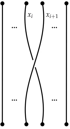
projection line. As particles move in time, and their strands cross one another, the projection of the strands onto the projection line will change; we update the enumeration accordingly. For 1 ≤ _i < _{n, we let} σ_{i denote}

the braid consisting of a single crossing given by passing the ith strand behind the (i+1)st strand (Figure 2.2). Viewed from above, the braid σi

corresponds to a clockwise half-twist of strandsiandi+1. Conversely, we letσ−₁1denote the single crossing given by passing theith strand in front of the(i+1)st strand.

xi xi+1

Figure 2.2: Illustration ofσi, the braid consisting of a single crossing given

by passing the ith strand behindxi the(i+1)st strandxi+1. We adopt the

convention of drawing our braids from top to bottom.

A topological braid is specified by a concatenation (product) of σi.

Fol-lowing the standard practice in braid literature, we adopt the convention

of composing our elements from left to right. Furthermore, we adopt the convention of drawing our braids from top to bottom.

Topological braids are classified up to isotopy. We say that two braids are isotopicif one can be deformed into the other through a continuous family of homeomorphisms.

Definition 2.2(braid group onnstrands). The isotopy classes of braids on

nstrands form a groupBn, called thebraid group on n strands.

The collection of braidsσi, 1 ≤ i < n, generate the braid groupBn. In fact,

Artin [44] showed that the braid groupBnadmits the following presentation:

Bn =

*

σ1,· · · ,σn−₁

σiσi+1σi =σi+1σiσi+1 for alli

σiσj =σjσi for all

i− _j

>1 +

.

Artin’s presentation gives the braid group an algebraic structure. Thus, a product ofσiwill sometimes be referred to as analgebraic braid.

For the remainder of this document, when we say braid, we will mean topological braid, unless otherwise specified.

2.3.2 Mapping class groups

Identifying a braid onnstrands with (an isotopy class of) a homeomorphism of ann-punctured disk confers several advantages.

First, it is intuitive to visualize the advection of an isotopy classcof a simple closed curve by a homeomorphism of ann-punctured disk. An isotopy class cthat encloses two or more punctures may stretch or fold, depending on the dynamics of the homeomorphism. This provides a topological parallel to the advection of material lines in a fluid. Isotopy classes that do not grow (or isotopy classes that grow least [36]) delineate coherent sets.

We will also note that the homeomorphism viewpoint will also be an im-portant tool in several of our proofs.

Definition 2.3(mapping class group). Themapping class group of a surface S,

denoted

Mod(S) =π0

Homeo+(S,∂S),

is the group of isotopy classes of elements of Homeo+(S,∂S), the group of orientation-preserving homeomorphisms onSthat restrict to the identity on ∂S, endowed with the compact-open topology.

These groups are discussed in detail by Farb and Margalit [40].

The braid group Bn is isomorphic to the mapping class group of an

n-punctured diskDn:

Bn ≈Mod(Dn) =π0

Homeo+(Dn,∂Dn)

. (2.1)

Under this isomorphism, each generator σi corresponds to the homotopy

class of a homeomorphism of Dn that has support a twice-punctured disk

and is given by a positive half-twist on this support [40, 45].

Unless otherwise specified, we will use the model ofDn given by the unit

disk centered at the origin, with npunctures arranged along thex-axis, so that they partition the interval[−_{1, 1]inton+1 equal segments.}

Nielsen-Thurston classification

The Nielsen-Thurston classification theorem characterizes mapping classes.

Theorem 2.4 (Nielsen-Thurston classification [40, 46]). Let g,n ≥ _{0. Each}

mapping class f ∈ _{Mod(Sg,n) is either periodic, reducible, or pseudo-Anosov.}

Further, pseudo-Anosov mapping classes are neither periodic nor reducible.

Definition 2.5(essential curve). A closed curve is calledessentialif it is not homotopic to a point, a puncture, or a boundary component.

Definition 2.6 (geometric intersection number). The geometric intersection

numberbetween free homotopy classesaandbof simple closed curves in a surfaceSis the minimal number of intersection points between a represen-tative curve in the classaand a representative curve in the classb.

Remark 2.7([40]). The geometric intersection number i(a,b) is realized by

geodesic representatives ofaandb.

Definition 2.8(reducible). A mapping class f ∈ _{Mod(S) isreducibleif there}

is a non-empty set C = {_c1,· · · _,ck} _{of isotopy classes of essential simple}

closed curves inSso that the geometric intersection numberi(ci,cj) = 0 for

all i and j and so that{_f(cj)} ₌ {_cj}_{. The collection}C _{is called a reduction}

systemfor f.

We are particularly interested in reducible maps defined onDn. While the

reduction system of a map onDnmay be complicated, every reducible map

is conjugate to a braid with a reduction system consisting of a family of geometric ellipses centered on the axis through the punctures [37–39]. We say that a curve isroundif it is isotopic to a geometric ellipse inDn. We say

that a reduction systemC isround‡if each curve inC is round.

In general, a reducible map may admit many reduction systems. A reduction system C is anadequate reduction system for a mapping class f ∈ _{Mod(S) if}

cuttingSalongC decomposesfso that the restriction of fto each component ofS\C _{is either finite-order or pseudo-Anosov [48].}

Birman, Lubotzky, and McCarthy [48] showed that every reducible map f has anessential reduction system, denoted ERS(f), such that

1. every curve§c ∈_{ERS(f)is preserved by some power of f;}

‡

Lee and Lee [47] refer to such a reduction system as astandard reduction system.

§

2. any curve that has non-trivial geometric intersection with some curve c∈_{ERS(f)is not preserved by any power of f.}

The essential reduction system of a map f is unique (up to isotopy). Further-more, the essential reduction system of f is a minimal adequate reduction system of f, with respect to inclusion.

The essential reduction system for a mapping class f ∈_{Mod(S)is sometimes}

called acanonical reduction system, which is defined by Farb and Margalit [40] as the intersection of all maximal (with respect to inclusion) reduction sys-tems for f. The two definitions are equivalent [40, 48].

Remark 2.9([39]). With the isomorphism (2.1) in mind, we will sometimes

use the term braid to refer to a mapping class.

We say that a braid β is periodic if for some integer r, the rth power βr is isotopic to a full Dehn twist on the boundary of then-punctured diskDn.

A braid is reducible if its corresponding mapping class is reducible. Simi-larly, a braid ispseudo-Anosovif its corresponding mapping class is pseudo-Anosov.

Remark 2.10. An essential reduction system ERS(β) is non-empty if and

only ifβis reducible and non-periodic [48].

2.3.3 Automorphisms of a free group

In order to provide an interpretation of the Burau representation as a cov-ering space action in the next section, we use the faithful representation of the braid group Bn as a group of (right) automorphisms of a free group

Fn =hx1,· · · ,xnionngenerators [44, 49].

The representationξ: Bn →Aut(Fn)is induced by mapping a generatorσi

of the braid group Bn to the automorphism (σi)ξof a free groupFn, given

by

xi→ xixi+1x

−₁

i ,

xi+1→ xi,

Remark 2.11. The automorphism(σ−_i1)ξis given by xi→ xi+1,

xi+1→ x

−₁

i+1xixi+1,

xj→ xj if j,i,i+1.

2.4 Application to the analysis of flows

In this section, we detect dynamically distinct regions as levelsets of an eigenvector of the (unreduced) Burau matrix corresponding to the motion of the particles. To do so, we introduce the Burau representation, which is an example of a Magnus representation [44]. We interpret the Burau representation as a covering space action. Following this, we show that when a reducible pure braidαhas a round reduction system C, the Burau matrixB(α)(t)has an eigenvector that is piecewise constant on the interior of the reduction curvescj ∈ C. We conclude that for any reducible braidβ,

the Burau matrix B(β)(t ≈ _{1) has an eigenvector that is approximately}

piecewise-constant on components of its Nielsen-Thurston decomposition.

2.4.1 (Unreduced) Burau representation

Matrix representation

The Burau representation is a homomorphism ρn :Bn →GLn(Λ),

with Λ := Z[t±]. The matrix representation allow us to examine the dy-namics of a motion of particles through a study of eigenvectors. There are two forms of the Burau representation, the reduced and unreduced. Our analysis focuses on the unreduced Burau representation, which is given by mapping a generatorσiofBn to the block matrix

B(σi) (t) :=Ii−₁⊕

     

1−_{t t}

1 0

     

⊕_{In−i−1. (2.2)}

We writeB(α)(t)for the Burau matrix for the braidαwith parametert. We note that

[B(σi) (t)]

−₁

=Ii−₁⊕

     

0 1

t−1 1−_t−1

     

It can be verified that

[B(σi) (t)]

−₁

=Bσ−_i1(t).

The constant vector (1,· · · _{, 1) generates an invariant subspace of the}

ma-trices B(σi) (t). The reduced Burau representation is obtained by taking the

quotient.

Unless otherwise specified, in this document, when we say Burau represen-tation, we will mean the unreduced Burau representation.

The Burau representation is known to be not faithful forn≥_{5 [50, 51]. The}

case n = 4 remains open. Church and Farb [52] that the kernel ofρn is in

fact quite large forn≥_{6. In our experience, the unfaithfulness of the Burau}

representation has not been an impediment to extracting coherent sets from physical systems.

Remark 2.12. For every constant vector v, we have thatB(σ)(t)v = v for

every braidσand allt. Proof.

It is sufficient to prove this result for the generatorsB(σi)(t).

Whenv1 =v2, we have that

     

1−_{t t}

1 0             v1 v2      =      

(1−_t)v1+tv2

v1      =       v1 v1      . Thus,

B(σ_i) (t) :=Ii−₁⊕

     

1−_{t t}

1 0      

⊕_In−i−1

fixes constant vectors.

Covering space action

The Burau representation has a topological interpretation as a covering space action [53, 54].

For 1≤ _j≤_{n, letpj =} j

n+1, and consider ann-punctured disk

Dn =

z− 1

2 ≤₁ \

Fix a basepointp0 ∈ ∂Dn, and around each puncturepj, take a small

clock-wise loopxj, such that xj(0) = xj(1) = p0. Then π1(Dn,p0)is freely

gener-ated by the set of homotopy classes[xj].

Let τ : π1(Dn,p0) → Z be the epimorphism generated by τ

[x_j] = 1 for 1 ≤ _j ≤ _{n. The kernel of}τ _{consists of all words in}{_xj}n

j=1 whose exponent

sum is zero. This is a normal subgroup. So we can define a covering space p: De_n →D_n corresponding to the kernel ofτ.

LetFbe the fiber above the basepointp0, and consider the relative homology

groupH1

e Dn,F

. By construction, the deck group ofDe_nis isomorphic toZ. Call its generatort. Then H1

e Dn,F

is free and n-dimensional as a module overΛ=Z[t±]. The action ofBnonH1

e Dn,F

gives the (unreduced) Burau representation.

Example 2.13. We consider the casen=3.

Let D3 denote a thrice-punctured disk with punctures p1, p2, p3. Fix a

basepoint p0 ∈ ∂D3. Let x1, x2, x3 be small clockwise loops in (D3,p0),

enclosing puncturesp1,p2,p3, respectively.

As aΛ-module, the homology groupH1

e D3,F

has three generators, ˜x₁, ˜x2,

˜

x3, given by the lifts of x1,x2,x3, each ˜xibeginning at some fixed basepoint

˜ p0∈ F.

The generatorσ1induces a map on the fundamental groupπ1(D3,p0)

send-ingx₁tox₁x2x−₁1. Thus,σ1induces a map (σ1)∗ on homology that sends ˜x₁

to the lift ofx1x2x−₁1, which is

˜

x1+t˜x2−t˜x1 = (1−t)x˜1+t˜x2.

Similarly,

(σ₁)∗(x˜₂) =x˜₁,

(σ₁)∗(x˜₃) =x˜₃.

LetB1be the matrix whose (i, j)th entry is the coefficient of ˜xjin the image

(σ₁)∗(x˜_i). Then

B1 =

          

1−_{t t 0}

1 0 0

0 0 1

          

Performing the same analysis for the generatorσ2, we have

(σ2)∗(x˜₁) =x˜₁,

(σ₂)∗(x˜₂) = (1−t)x˜₂+x˜₃,

(σ2)∗(x˜₃) =x˜₂.

As before, we letB2be the matrix whose(i,j)th entry is the coefficient of ˜xj

in the image of(σ2)∗(x˜_i). Then

B1 =

          

1 0 0

0 1−_{t t}

0 1 0

          

=B(σ2)(t).

Relationship to algebraic intersection numbers

The matrix entries of the Burau representation can also be interpreted as algebraic intersection numbers [50, 55].

Definition 2.14 (algebraic intersection number [40]). Let a and b be a pair

of transverse, oriented, simple closed curves in a surface S. The algebraic intersection number ˆi(a,b) is defined as the sum of the indices of the inter-section points ofa and b, where an intersection point is of index+1 when the orientation of the intersection agrees with the intersection of Sand −₁

otherwise.

Remark 2.15([40]). The algebraic intersection number ˆi(a,b) depends only

on the homology classes ofaandb.

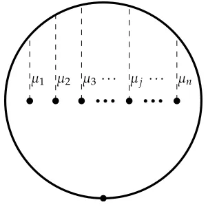
Letµj, 1≤ j≤n, be the arcs shown in Figure 2.3.

We define a mapR ωj : H1

e Dn,F

→ Λ_{on a homology classa} ∈ _H1Den,F

by setting

Z

a

ωj =

X

k∈Z

tk ˆia,tkµj

, where ˆia,tkµj

is the algebraic intersection number of the arcsaandtkµjin

the covering spaceDe_n.

Then the Burau matrixB(β)of a braidβ ∈_{Bnhas entries given by}

B(β) (t)i,j =

Z

µ1 µ2 µ3 · · · µj · · · µn

Figure 2.3: Illustration ofµjinDe_n.

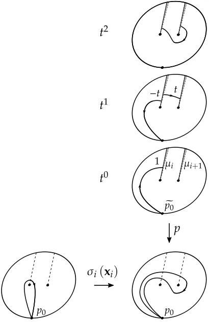
Example 2.16. In Figures 2.4 and 2.5, we consider the image of the clockwise

loops x_i and x_i+1, respectively, under the braidσi. We consider the lifts of

σi(xi)andσi(xi+1)to the cyclic covering spaceDe_n. The oriented intersections of the lifts with the arcsµi,t1µi,t2µiandµi+1,t1µi+1,t2µi+1(illustrated by the

solid lines in each copy of Dn inDe_n) give the matrix entries for the Burau matrixB(σi)(t)in Equation (2.2).

In particular, the lift ofσi(xi)begins atpe0, intersectsµionce, then intersects tµi+1 once, ascends to the next copy of Dn before descending again, upon

which it intersects tµi in the opposite orientation, and ends at tpe0. (See Figure 2.4 for an illustration.) This corresponds to theith row of the Burau matrix B(σi)(t), which has non-trivial entries 1−t and tin columns i and

i+1, respectively.

The lift of σi(xi+1) begins at pe0, intersects µi once, and ends at tpe0. (See Figure 2.5 for an illustration.) This corresponds to the (i+1)st row of the Burau matrixB(σi)(t), which has a single non-trivial entry consisting of 1 in

columni.

Example 2.17(tubular braid). We use the notation of Band and Boyland [56]

and refer to the braid that moves the group ofη1consecutive strands starting

at strandibehind the group ofη2consecutive strands starting at strandi+η1

as

σi,η1,η2 =

σi+η₁−₁· · ·σ_i+η₁+η₂−₂ σ_i+η₁−₂· · ·σ_i+η₁+η₂−₃

· · ·σ_i· · ·σ_i+η

2−1

σi(xi)

p t2

t1

t0

µi µi+1

1 −_t t

p0 p0

e

p0

Figure 2.4: Illustration ofσi(xi)and its lift to the covering spacep: De_n →D_n.

By considering lifts of the images of the loops xj underσi,η1,η2 to the cyclic coverDe_n (see Figure 2.7), one can prove that the Burau matrixB(σi,η

1,η2)of the braidσi,η1,η2 is a block matrix of the form:

Ii−₁⊕

                 

1−_{t t}−_t2 · · · _tη2−1−_tη2 _tη2 · · · ₀

..

. ... ... . ..

1−_{t t}−_t2 · · · _tη2−1−_tη2 _0η

1 · · · tη2

Iη2 0

                 

⊕_In−i−η

1−η2+1.

Given a block vectorv= (v1,· · · ,vn), with

vj =

        

b fori≤ _j<_i+η_1,

σi(xi+1)

p t2

t1

t0

µi µi+1

1

p0 p0

e

p0

Figure 2.5: Illustration ofσi(xi+1) and its lift to the covering spacep : De_n → Dn.

we have that

Bσi,η1,η2 (t)                                                                 v1 .. . vi−₁

b .. . b c .. . c vi+η₁+η₂

.. . vn                                                                 =                                                                 v1 .. . vi−₁

b(1−_tη2_{) +ct}η2 ..

.

b(1−_tη2_{) +ct}η2 b

.. . b vi+η₁+η₂

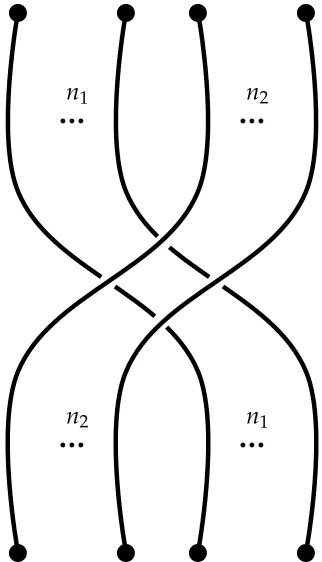
n1 n2

n2 n1

Figure 2.6: Illustration of a braid corresponding toσi,η1,η2

So whentis anη2th root of unity, the Burau matrixB(σ)(t)is a permutation

of the blocks indexed by i ≤ µ < _i+η_{1 and i+}η₁ ≤ ν < _i+η₁₊η_{2 and}

the identity elsewhere. For all othert, the Burau matrixB(σ)(t)maps block vectorsvthat are piecewise-constant on the blocks indexed byi≤µ <_i+η₁

andi+η₁ ≤ ν <_i+η₁₊η_{2to block vectors that are piecewise-constant on}

the blocks indexed by indexed byi≤ν <_i+η_2andi+η₁≤µ <_i+η₁₊η_2.

Performing a similar analysis, one can show that the Burau matrixB(σ−_i,η1 1,η2)(t) of the inverseσ−_i,η1

1,η2 is a block matrix of the form

Ii−₁⊕

                 

0η2 Iη1

t−η1 · · · _{0 1}−_t−1 _t−1−_t−2 · · · _t−η1−1−_tη1

. .. .._. .._. .._.

0 · · · _t−η1 ₁−_t−1 _t−1−_t−2 · · · _t−η1−1−_tη1                  

⊕_In−1−η

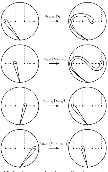
σi,n1,n2(xi)

σi,n1,n2

xi+n1−1

σi,n1,n2

xi+n1

σi,n1,n2

x_i+n1+n2−1

Figure 2.7: Covering space action of σ_i,η1,η2. If i ≤ _j < _i+η_{1 (top two}

rows), the lift ofσi,η1,η2

xj

toDe_n begins atp_e0and goes up, intersecting the arcsµi,tµi+1,· · · ,tη2−1µi+η2; it then intersectstη2µη2+j−i+1before going back down, upon which it intersects the arcstη2µ

i+η₂,tη2−1µi+η₂−₁,· · · ,tµ_i in the

opposite direction, and ends attpe0. Ifi+η1 ≤ j < i+η1+η2 (bottom two rows), the lift ofσi,η1,η2

xj

and

Bσ−_i,η1 1,η2

(t)                                                                 v1 .. . vi−₁

b .. . b c .. . c vi+η1+η2

.. . vn                                                                 =                                                                 v1 .. . vi−₁

c .. . c

bt−η1_+c(1−_t−η1₎ ..

.

bt−η1_+c(1−_t−η1₎ vi+η1+η2

.. . vn                                                                 .

Example 2.17 is an example of atubular braid[57]. Decomposition of reducible braids

Next, we show that a reducible braid with a round reduction system can be decomposed as a product of braiding between tubular braidsσε_i((<sub>`</sub>`₎)_,η

1(`),η2(`) with trivial braiding within tubes, wherei(`),η1(`),η2(`)are positive

inte-gers andε(`) =±_{1, followed by a product of braiding within tubular braids}

with trivial braiding between tubes.

Note that given any reduction systemC of a reducible braidα∈_{Bn, we can}

always choose a non-empty, non-nested subset Cext consisting only of the

outermost (i.e., exterior) curves ofC.

Lemma 2.18. Let α ∈ _{Bn be a reducible braid that preserves a non-nested round}

reduction systemC. For each puncture pr of Dn not enclosed by any curve of C,

extendC by adding a round curve crenclosing the single puncture pr. Let k be the

number of curves in (the newly extended) C. Then there exists a finite sequence of tuples (i(`),η1(`),η2(`),ε(`)) of integers and a finite sequence of braids αj,

1 ≤ _j ≤ _{k, each} α_{j supported on the punctured disk with boundary given by the}

curve cj ∈C, such that

α=Y

`

σε(`)

i(`),η<sub>1</sub>(`),η₂(`)·

k

Y

j=1

Proof.

LetEjdenote the punctured disk enclosed by the circlecj∈ C, enumerating

the disksEjin order along the axis through the punctures. Let

b

Dk =Dn\ k

[

j=1

Ej.

Thenαinduces an automorphismbαonDbk.

If we collapse each hole of Db_k to a puncture, we can regard Db_k as a k-punctured disk. So the braidbαcan be given by a sequence of Artin generators for the braid groupBk:

bα= Y

bσ

ε` a<sub>`</sub>,

where 1 ≤ _{a`</sub> < <sub>k and</sub> ε<sub>` =} ±_{1 for all} `. Viewed from above, each

gen-erator bσa` corresponds to a clockwise half-twist interchanging the holes obtained by removing Ea<sub>`</sub> and Ea_`+1. Thus, each bσ

ε`

a_` specifies a tuple

(i(`),η1(`),η2(`),ε(`)), given by the minimum index of the punctures in

Ea_{`</sub>, the number of punctures inEa<sub>`}, the number of punctures inEa_`+1, and

the direction of the half-twist, respectively.

Lettingαj=α|Ejdenote the restriction ofαtoEj, this completes the decom-position.

Definition 2.19(piecewise-constant vector). LetC be a non-empty finite

col-lection of pairwise-disjoint non-trivial simple closed curves such that each curvecj∈C encloses at least one puncture of ann-punctured diskDn.

Cut-ting then-punctured diskDnalong the curvescj∈C, we obtain a collection

E of path-components. We say that a vector v = (v1,· · · ,vn) is

piecewise-constant on components of (Dn,C) if v` = v`0 whenever the corresponding puncturesp_{`</sub>andp<sub>`}0 belong to the same path-component inE.

LetEjdenote the punctured disk enclosed by the curvecj ∈C. We say that

Example 2.20. LetC ={_c1,c2,c3,c4}_{be a finite collection of pairwise-disjoint}

simple closed curves such that:

• _{the curvec1encloses puncturesp1,}· · · _,pi−1, • _{the curvec2encloses puncturespi,}· · · _,pi+η

1−1,

• _{the curvec3encloses puncturespi+η}

1,· · · ,pi+η1+η2−1, and

• _{the curvec4encloses puncturespi+η}

1+η2,· · · ,pn.

Ifvbe a vector that is piecewise-constant on components of(Dn,C), then by

Example 2.17, the imageB(σ_i,η1,η2)(t)vis also piecewise-constant on compo-nents of(Dn,σi,η1,η2(C))for allt.

Lemma 2.21. Consider the braid

α=

m

Y

`=1

σε(`)

i(`),η<sub>1</sub>(`),η₂(`)·

k

Y

j=1

αj,

from Equation (2.3), where(i(`),η1(`),η2(`),ε(`))andαjare given in the proof of

Lemma 2.18. LetC be the non-nested family of round simple closed curves given in the hypothesis of Lemma 2.18. If v be a block vector inCn such that v is piecewise-constant on components of(Dn,C), then the image B(α)(t)v is piecewise-constant

on components of(Dn,α(C)).

Proof.

As a corollary of Remark 2.12, for each 1≤ _j≤_{k, we have thatB(}α_j)(t)v=v

for all vectorsvthat are constant onEj. So

       

k

Y

j=1

B(α_j)(t)        

v=v.

Thus, without loss of generality, we need only consider braids of the form α=Qm

`=1σi(`),η₁(`),η<sub>2</sub>(`).

We prove the proposition by induction onm≥_1.¶

¶

We note that an intermediate braid Qm0

`=1σi(`),η1(`),η2(`), where 1 ≤ m

0 _<

The base case is given by Example 2.17. For the inductive case, we considerα = Qm

`=1σi(`),η₁(`),η<sub>2</sub>(`) and the corre-sponding Burau matrices

B(α)(t) =

m

Y

`=1

Bσi(`),η<sub>1</sub>(`),η₂(`)

(t).

Letα0=Qm−1

`=1 σi(`),η1(`),η2(`). By the inductive hypothesis, w0 =B(σ0)(t)v

is piecewise-constant on components of(Dn,α0(C)).

Furthermore, by construction (Lemma 2.18), the image w0 is piecewise-constant on the component containing i(m) and on the component con-taining i(m) +η1(m). So applying the base case (Example 2.17), we have

that

B(σ_i(m),η₁(m),η₂(m))(t)w

0

is piecewise-constant on components of(Dn,α(C)).

This proves the inductive hypothesis and thus concludes our proof.

Piecewise-constant eigenvectors

Combining Lemmata 2.18 and 2.21, we have the following corollary:

Corollary 2.22. Letαbe a reducible braid with a round reduction systemC. Let

V be a block vector in Cn that is piecewise-constant on components of (Dn,C).

Then the image B(α)(t)V is a block vector, piecewise-constant on components of (Dn,C) = (Dn,α(C)).

Suppose the block vectorVhas valueVjonEj. Then we can write

B(α)(t)             V1 .. . Vk             =              Pk

j=1V1p1,j(t)

.. . Pk

j=1Vkpk,j(t)

             ,

For each fixedt, the matrix

P=            

p1,1(t) · · · p1,k(t)

..

. . .. ... pk,1(t) · · · pk,k(t)

           

has an eigenpair(λ,v), withλ∈C_andv∈Ck_{. Letting the jth block ofVbe}

given by the jth entry ofv, we have that(λ,V)is an eigenpair ofB(α)(t). Now, when αis additionally a pure braid, the Burau matrixB(α)(1) is the identity. Since the Burau representation is continuous intatt =1, then for everyε >0, the Gershgorin circle theorem guarantees that there existsδ >0 such that for alltsatisfying|_t−₁|< δ, we have that|λ−₁|< ε. (See Lemma

2.26 for guidance on the choice oft.) Thus,

Proposition 2.23. Letαbe a reducible pure braid with round reduction systemC.

Then there exists δ > 0such that for all t satisfying |_t−₁| < δ, we have that the

Burau matrix B(α)(t)has an eigenvector that is piecewise constant on(Dn,C).

Using that every reducible braid is conjugate to a braid with a round reduc-tion system, we now show that every reducible pure braid has an eigenvector that is almost piecewise-constant on its components.

Proposition 2.24. Letβ∈ _{Bnbe a reducible pure braid with a reduction system}C_β.

For each ε > 0, there exists t ∈ C, such that the Burau matrix B(β_{)(t) has an}

eigenvector vε(t) = v(t) +e(t), where v(t) is a vector that is piecewise-constant

on(Dn,Cβ), and e(t)is a matrix whose entries are bounded byε, with

ei,j(t)

< ε for all1≤_i,j≤_n.

Proof.

There exists a braidαconjugate toβinBn, withβ=γ−1αγfor someγ∈Bn,

such thatαhas a round reduction systemC =γ(C_β), whose curves are given byγ(cj), for some curvecj ∈ Cβ, where we considerγas an automorphism

Let their corresponding Burau matrices be denoted A(t) =B(α)(t),

B(t) =B(β)(t),

C(t) =B(γ)(t).

ThenB(t) =C(t)A(t)C(t)−1. (Note that we compose braids from left to right but compose matrices from right to left.)

SinceC(t) is continuous int att = 1, there exists δC > 0 such that for allt

satisfying|_t−₁|< δ_{C, we have that}

C(t)−_C(1)

< ε. (2.4)

(See Lemma 2.26.)

By Proposition 2.23, sinceαis a reducible pure braid with a round reduction system C, there exists δA > 0 such that for all t satisfying |t−1| < δA, the

Burau matrix A(t) has an eigenvector v(t) that is piecewise-constant on (Dn,C).

So for alltwithinδ =min{δ_A,δ_C}_{of one, we have that Equation (2.4) holds}

and thatA(t)has an eigenvectorv(t)that is piecewise-constant on(Dn,C).

Without loss of generality, assume v(t)

= 1. Note that C(t)v(t) is an eigenvector ofB(t),

B(t)C(t)v(t) =C(t)A(t)C(t)−1C(t)v(t) =C(t)A(t)v(t) = C(t)v(t),

but not necessarily piecewise-constant on(Dn,γ−1(C)), whereγ−1(C)is the

reduction systemCβ forβ. On the other hand, sinceC(1)is a permutation

matrix, the vector C(1)v(t) is piecewise-constant on (Dn,γ−1(C)) but not

necessarily an eigenvector ofB(t). Since

C(t)v(t)−_C(1)v(t) ≤

C(t)−_C(1) v(t)

=

C(t)−_C(1) < ε,

the vectorC(t)v(t)satisfies the proposition.

Remark 2.25. Since the Burau representation is not faithful, we cannot

Continuity of the Burau representation

Since the Burau representation is continuous in t at t = 1, then for every braid γ and every ε > 0, there exists t such that B( γ)(t)−B(γ)(1)

< ε. Informally, since the Burau matrixB(γ)(1)is a permutation matrix, then for t ≈ _{1, the Burau matrix B(}γ_{)(t) is approximately a permutation matrix. In}

the following lemma, we quantify this approximation.

Lemma 2.26. Letγ∈ _{Bn, with}γ ₌QL

j=1σaj. Then for all0<|t|<1, we have

B(γ)(t)−_B(γ₎₍₁₎

≤L(n+1) L−1

2

√

2|₁−_t|_,

wherek·k_{is the Frobenius matrix norm,}

k_Bk₌

        n X

j=1 n

X

i=1

bi,j

2         1/2 . Proof.

For each generatorσi∈Bn andt∈Csuch that|t| ≤1, we have

B(σi)(t)

2

=n−₁₊|₁−_t|2₊|_t|2≤_n+1,

B(σi)(1)

2 =n, and

B(σi)(t)−B(σi)(1)

2

=2|₁−_t|2_.

So for a braidγ =QL

j=1σaj, we have that L Y

j=1

B(σaj)(t)−

L

Y

j=1

B(σaj)(1) , = L X

j=1

       

j−₁

Y

i=1

B(σaj)(t)        

·_B(σ_a

j)(t)−B(σaj)(1) ·         L Y

i=j+1

B(σai)(1)         , ≤ L X

j=1

       

j−₁

Y

i=1

B(σaj)(t)        

·_B(σ_a

j)(t)−B(σaj)(1) ·         L Y

i=j+1

B(σai)(1)         , ≤ L X

j=1

       

j−₁

Y

i=1

B(σaj)(t)        

·_B(σ

aj)(t)−B(σaj)(1) ·         L Y

i=j+1

B(σai)(1)         ,

≤_L(n+1)L

−1 2

√

Corollary 2.27. Letε >0. For t∈C, with₀<|_t|<_{1, such that}

|₁−_t|< √

2ε

2L (n+1)

−L−1

2 _. Then_B(γ_)(t)−B(γ₎₍₁₎

< ε.

2.4.2 Numerical implementation

In the following section, we compute the Burau matrix for two different dynamical systems and visualize corresponding eigenvectors whose level-sets correspond to components of the Nielsen-Thurston decomposition. Given trajectoriesxj : [0, 1] → R2×[0, 1], 1≤ j≤ n, we use braidlab [43] to

compute the algebraic braidβcorresponding to the motion of the particles, with respect to some fixed projection line. Prior to computing the algebraic braid, some preprocessing and extra consideration are necessary.

(i) Resolving coincident projections. We note that when our initial

po-sitions are given by grid points of a regular grid, it can be helpful to perturb the initial positions and/or choose a projection line that is not parallel to the grid lines (i.e., not thex- ory-axis). This will help resolve some coincident trajectories in the projection, allowing the algebraic braid (i.e., sequence ofσi) to be computed.

(ii) Enforcing closure. In general, sets of trajectories do not form true

geometric braids, since the set of particle positions at initial time and the set of particle positions at final time are not necessarily the same. In such a setting, changing the projection line (to form an algebraic braid) will not necessarily result in a conjugate braid [41, 42]. To rectify this, in the examples that follow, for each trajectoryxj(t0),· · ·xj(tN)

, we append the initial positionxj(t0)to form the closed trajectory

xj(t0),· · ·xj(tN),xj(t0)

.

By enforcing closure in a way that yields a pure braid, we are able to apply Proposition 2.24 to extract components of a reducible braid.

Once the algebraic braid is computed, we map each generator σi of the

algebraic braid to its corresponding Burau matrix, given in Equation (2.2), and we instantiate the Burau matrices with a fixed real-valued tsuch that t≈_{1. (Corollary 2.27 can be used to choose the value of t.) The product}

Q

B(σb_`)(t≈1), whereβ=

Q

`σb<sub>`</sub>, is the Burau matrix corresponding to the

braid of trajectories.

We should note that an eigenvector found in this manner may not necessarily delineate all components of a reducible braid. In fact, for a pure braid β, all vectors of the form (0,· · · _{, 0, 1, 0,}· · · _{, 0) are eigenvectors of B(}β_{)(1). In}

practice, these vectors are easy to distinguish from eigenvectors that reveal dynamical structure.

The assiduous reader may note that most theorems in this document were proven for the more general caset∈C. These proofs also hold for_t∈R. In

practice, instantiating the Burau matrices to a real-valuedt ∈ R_{halves the}

number of arithmetic operations required, and no fidelity is forfeited.

2.5 Examples

We demonstrate the relevance of our contributions on two examples: the blinking vortex flow and the (modified) Duffing oscillator.

2.5.1 Blinking vortex flow

The blinking vortex flow was introduced by Aref as an idealization of stir-ring [44]. The flow is given by a pair of vortices separated by a finite distance, blinking on and off periodically in an alternating fashion in an incompressible, inviscid fluid. We consider a modified version of this flow in an unbounded domain (modeled on the complex plane).

The velocity field due to a single point vortex located atx=aon thex-axis is given by

˙ r=0, ˙ θ= Γ

-1.5 -1 -0.5 0 0.5 1 1.5 -1.5

-1 -0.5 0 0.5 1 1.5

-1.5 -1 -0.5 0 0.5 1 1.5

-1.5 -1 -0.5 0 0.5 1 1.5

-1.5 -1 -0.5 0 0.5 1 1.5

-1.5 -1 -0.5 0 0.5 1 1.5

-1.5 -1 -0.5 0 0.5 1 1.5

-1.5 -1 -0.5 0 0.5 1 1.5

-1.5 -1 -0.5 0 0.5 1 1.5

-1.5 -1 -0.5 0 0.5 1 1.5

-1.5 -1 -0.5 0 0.5 1 1.5

-1.5 -1 -0.5 0 0.5 1 1.5

-1.5 -1 -0.5 0 0.5 1 1.5

-1.5 -1 -0.5 0 0.5 1 1.5

-1.5 -1 -0.5 0 0.5 1 1.5

-1.5 -1 -0.5 0 0.5 1 1.5

whereΓis the strength of the vortex, andr= p(x−_a)2_+y2_{is the distance}

to the center of the vortex.

The mapping, in dimensionless form [58], induced by two identical vortices atξi =±a, each acting for timeT, is given by thetwist map

     

x y

     

7→

     

ξi+ (x−ξi)cos∆θ−ysin∆θ

(x−ξ_i)sin∆θ_+ycos∆θ

     , where ∆θ = _rµ2, withµ = _2πaΓT2, andr =

q

(x−_xi)2_+y2_{. The parameter µ}

is the flow strength, and its value controls the behavior of the system. We make distances dimensionless with respect to a and place the vortices at ξi =±1.

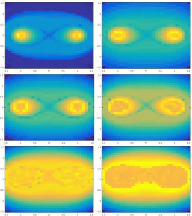
When both vortices act simultaneously (T = 0, µ = 0), the system is in-tegrable. We perturb the system by increasing µ from zero and study the Poincar´e sectionst =kT,k ∈Z_{(See Figure 2.8). Chaotic regions appear for}

all µ > 0 [59]. For small values of µ, small chaotic regions exist near the elliptic and hyperbolic points. Asµincreases, the size of the chaotic regions grow, destroying confining KAM surfaces as the chaotic regions merge. Using the methods described above, we give eigenvectors for the blinking vortex flow forµ=0.01, 0.05, 0.10, 0.20, 0.35, 0.50 in Figure 2.9.

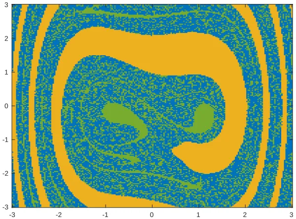
2.5.2 Modified Duffing oscillator

In this example, we study a modified Duffing oscillator, given by ˙

x= y+αcos(ωt), ˙

y=x1−_x2−δy₊γ_cos(ωt)_, (2.5)

withα=0.1,γ =0.14,δ=0.08,ω=1.

This compressible system is also studied by Allshouse and Thiffeault [36] with the same parameters as an example a system with two primary regions of mixing: (i) the limit cycle and its basin of attraction (yellow in Figure 2.10) and (ii) the rest of the domain (blue/green).

-1.5 -1 -0.5 0 0.5 1 1.5 -1.5

-1 -0.5 0 0.5 1 1.5

-1.5 -1 -0.5 0 0.5 1 1.5

-1.5 -1 -0.5 0 0.5 1 1.5

-1.5 -1 -0.5 0 0.5 1 1.5

-1.5 -1 -0.5 0 0.5 1 1.5

-1.5 -1 -0.5 0 0.5 1 1.5

-1.5 -1 -0.5 0 0.5 1 1.5

-1.5 -1 -0.5 0 0.5 1 1.5

-1.5 -1 -0.5 0 0.5 1 1.5

-1.5 -1 -0.5 0 0.5 1 1.5

-1.5 -1 -0.5 0 0.5 1 1.5

Figure 2.9: Eigenvectors of Burau matrix computed from trajectories of Aref’s blinking vortex flow; from left to right, and top to bottom: µ=0.01, 0.05, 0.10, 0.20, 0.35, 0.50.

We say that a limit cycle isstable(orattracting) if all neighboring trajectories approach the limit cycle. Otherwise, we say that the limit cycle isunstable. A stable limit cycle is an example of an attractor.