Web matrices: structural properties and
generating combinatorial identities
Mark Dukes
Computer & Information Sciences University of Strathclyde
Glasgow, G1 1XH, UK.
Chris D. White
School of Physics and AstronomyUniversity of Glasgow Glasgow, G12 8QQ, UK
[email protected] Submitted: Oct 13, 2015; Accepted: Feb 14, 2016; Published: Mar 4, 2016
Mathematics Subject Classifications: 05A05, 05A19, 05C50
Abstract
In this paper we present new results for the combinatorics of web diagrams and web worlds. These are discrete objects that arise in the physics of calculating scattering amplitudes in non-abelian gauge theories. Web-colouring and web-mixing matrices (collectively known as web matrices) are indexed by ordered pairs of web-diagrams and contain information relating the number of colourings of the first web diagram that will produce the second diagram.
We introduce the black diamond product on power series and show how it de-termines the web-colouring matrix of disjoint web worlds. Furthermore, we show that combining known physical results with the black diamond product gives a new technique for generating combinatorial identities. Due to the complicated action of the product on power series, the resulting identities appear highly non-trivial.
We present two results to explain repeated entries that appear in the web ma-trices. The first of these shows how diagonal web matrix entries will be the same if the comparability graphs of their associated decomposition posets are the same. The second result concerns general repeated entries in conjunction with a flipping operation on web diagrams.
We present a combinatorial proof of idempotency of the web-mixing matrices, previously established using physical arguments only. We also show how the entries of the square of the web-colouring matrix can be achieved by a linear transformation that maps the standard basis for formal power series in one variable to a sequence of polynomials. We look at one parameterized web world that is related to indecom-posable permutations and show how determining the web-colouring matrix entries in this case is equivalent to a combinatorics on words problem.
1
Introduction
Web diagrams are discrete objects that are subject to certain colouring and reconstruction operations, and arise in physics in the calculation of scattering amplitudes in non-abelian gauge theories [9, 16, 20]. A prominent example is the theory of quarks and gluons, Quan-tum Chromodynamics (QCD), which is of great topical relevance given its application to current experiments such as the Large Hadron Collider.
Whilst some properties of web-mixing matrices have been established from a physics point of view [9, 12], a fully general understanding of their structure and properties remains elusive. Web-colouring and web-mixing matrices admit a purely combinatorial definition and this provides an alternative framework to the physical picture to elucidate their properties. Our ultimate hope is that a detailed understanding of web diagrams and their matrices can be used to dramatically improve the precision of theoretical predictions for particle collider experiments.
The combinatorics of web diagrams and web matrices is an interesting study in its own right in that it combines parts of order theory, graph theory, and the theory of permutations in a new and novel way. Our seminal paper on the combinatorics of web diagrams [5] looked at these objects from several angles and has a companion physics paper [4] which explains how the results are pertinent to particle physics applications 1. We were able to show, for example, that for particular web diagrams, the diagonal entries of the web matrices corresponding to them depend on the generating function of the descent statistic formed by summing over the Jordan-H¨older set of all linear extensions of a web diagram’s decomposition poset (partially ordered set). We examined some special (parameterized) classes of web worlds which could be ‘exactly’ solved, and one of these saw the introduction of a new permutation statistic that did not seem to have been previously studied. Another result is that the number of different diagrams in a web world can be given by a hook-length style formula on its representation matrix.
Our aim in this study is not just to build on some of the results and directions that were initiated in [5], but to investigate some new aspects of these web diagrams that have not been explored before. Amongst these, we will give a combinatorial proof of idempotency of the web-mixing matrices that was originally established by way of a physics argument in Gardi and White [12, §3]. We will also introduce the black diamond product on power series and show how the web-colouring matrix of a web world whose web diagrams can be ‘partitioned’ (in a sense to be made precise later) depend on this black diamond product. Furthermore, we will show how a physics argument gives rise to a new technique for generating combinatorial identities using the black diamond product. We think that this technique is interesting in that it has the potential to generate quite unusual looking identities due to the black diamond product behaving in quite a complicated way on the power series in question.
We will concern ourself with the web diagrams that were defined in [5]2. Let P =
1For a recent introduction to the latter, see ref. [22].
{p1, . . . , pn} be a set of n pegs that are rooted to a plane. A web diagram D on P is a
set of 4-tuplesei = (ai, bi, ci, di) where the ei represents an edge between peg pai and peg
pbi for which the endpoint of ei on pegpai is thecith highest vertex on that peg from the
plane, and the endpoint of ei on peg bi is the dith highest vertex on that peg from the
plane. The labels of the endpoints of edges on each peg must be distinct, and this is taken care of in the formal definition, Definition 1. We will sometimes abuse the terminology by referring to ‘peg i’ in place of ‘peg pi’.
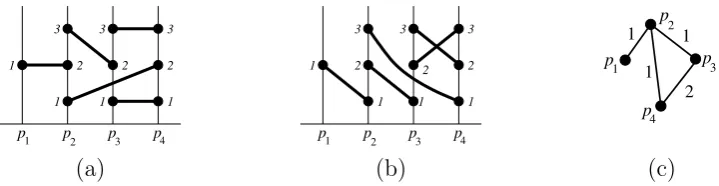
Two illustrations of web diagrams are given in Figure 1. The web world of a web diagram D is the set of all web diagrams that result from permuting the order in which vertices appear on a peg, and we usually denote it by W(D). The two web diagrams in Figure 1 are in the same web world. In the physics context in which such diagrams arise, the pegs represent quarks or gluons emanating from the interaction point, and the lines joining pegs correspond to additional gluons being radiated and absorbed. The conventional depiction of each web diagram is a so-called Feynman diagram, an example of which is shown on the left of Figure 2.
1
1 2 1
3
1 2
1 2
3 3
p p2 p3 p4
2 1
3
1 2 3 3
p1 p2 p3 p4
1 2
1
1
1
p4 p3 p2
1
2 1
p
(a) (b) (c)
Figure 1: Two examples of web diagrams in the same web world. Web diagrams (a) and (b) in this figure both have a single edge between ‘pegs’ p2 and p4. However the heights
of the endpoints differ in both diagrams. In (a) the heights of this edge on pegs p2 and
p4 are, respectively, 1 and 2. We represent this edge by the 4-tuple (2,4,1,2). In (b) the
heights of this edge are, respectively, 3 and 1. The edge in this diagram is represented by the 4-tuple (2,4,3,1). The web graph of the web world (to be defined in Section 2) containing the web diagrams is shown as (c).
To every web world W we associate two important matrices, M(W) and R(W), called
the web-colouring and web-mixing matrices, respectively. The entries of these matrices are indexed by ordered pairs of web diagrams, and contain information about colourings of the edges of the first web diagram that yield the second diagram under a construction determined by a colouring.
[image:3.595.118.478.301.394.2]In Section 5 we give two new results to explain the repeated entries that one notices occurring in web matrices. The first of theses results concerns diagonal entries and shows that if the comparability graphs of the decomposition posets of two web diagrams (that satisfy a further technical condition) are the same, then the diagonal entries on the web matrices for these two diagrams will be the same. The second result explains how the action of flipping a web diagram upside-down combines with the colouring and reconstruc-tion operareconstruc-tions on that same web diagram. In Secreconstruc-tion 6 we derive an expression for the entries of the square of a web-colouring matrix in terms of the entries of the web-colouring matrix, and give a combinatorial proof that the web-mixing matrices are idempotent.
Finally, in Section 7 we investigate a particular web world whose diagrams consist of only two pegs that have multiple edges between them. We show how they are related to indecomposable permutations and how calculating the entries of the web matrices for this web world reduces to a combinatorics on words problem.
2
Definitions and terminology
Let C[[x]] be the ring of formal power series in the variable x over the ring C. Given
f ∈ C[[x]] we will denote by [xi]f the coefficient of xi in f and we extend this notation
to the multivariate case. For integers a, b∈N leta∨b denote the maximum of a and b. If a6b, then let [a, b] ={a, a+ 1, . . . , b}.
Although web diagrams were defined in Section 1, we give here the formal specification in order to remove any uncertainty surrounding their definition.
Definition 1. A web diagram on n pegs having m edges is a collection D = {ej =
(aj, bj, cj, dj) : 1 6j 6m} of 4-tuples that satisfy the following properties:
(i) 16aj < bj 6n for all j ∈[1, m].
(ii) For i ∈ [1, n] let pi(D) be the number of j such that aj or bj equals i, that is, the
number of edges in D incident with peg i. Then the labels of the vertices on peg i
must be the first pi(D) positive integers, i.e.
{dj :bj =i} ∪ {cj :aj =i}= [1, pi(D)],
and no vertex on a peg can be both a left endpoint and a right endpoint of an edge, i.e.
{dj :bj =i} ∩ {cj :aj =i}=∅.
We write Pegs(D) = (p1(D), . . . , pn(D)). The labels of the pi(D) vertices on peg i when
read from bottom to top are (1, . . . , pi(D)).
Given a web diagram D= {ej = (aj, bj, cj, dj) : 1 6 j 6 m}, the set of pegs that are
incident with at least one edge is PegSet(D) ={a1, . . . , am, b1, . . . , bm}.
A web diagram D may be mapped to a simple graph G([1, n], E) where E(G) =
p2 p3
1
[image:5.595.140.460.71.176.2]p p4
Figure 2: The Feynman diagram corresponding to the web diagram of Figure 1(a) is illustrated on the left. The gluon lines correspond to the edges of the web diagram. The heights of the endpoints correspond to their distance from the meeting points of the the 4 arrowed lines. The ‘pegs and plane’ representation is shown to its right.
associated with a web world its web graph. The vertices of the web graph correspond to the pegs of the web diagram (all vertices on a peg in the web diagram are projected to a single vertex in the web graph). The edges of the web graph are labeled with the multiplicities of edges between the pegs in the web diagram. The web world that the web diagrams (a) and (b) of Figure 1 are members of is represented by the web graph (c).
Definition 2. LetD={ej = (xj, yj, aj, bj) : 16j 6m} and D0 ={e0j = (xj0, yj0, a0j, b0j) :
1 6 j 6 m0} be two web diagrams with PegSet(D),PegSet(D0) ⊆ {1, . . . , n}. The sum D⊕D0 is the web diagram obtained by placing the diagramD0 on top ofD;
D⊕D0 = D∪ {(xj0, yj0, a0j +px0
j(D), b
0
j+py0
j(D)) : 16j 6m
0}
.
If there exist two non-empty web diagrams E and F such that D = E⊕F then we say that D is decomposable. Otherwise we say that D is indecomposable.
Example 3. Consider the following two web diagrams: D1 = {(1,4,1,1),(2,6,1,2),
(2,6,2,1)} and D2 ={(1,2,1,1),(3,5,1,1),(5,6,2,1)}. For D1 we have
(p1(D1), . . . , p6(D1)) = (1,2,0,1,0,2)
and so
D1⊕D2
={(1,4,1,1),(2,6,1,2),(2,6,2,1)} ∪ {(1,2,1 +p1(D1),1 +p2(D1)),
(3,5,1 +p3(D1),1 +p5(D1)),(5,6,2 +p5(D1),1 +p6(D1))}
={(1,4,1,1),(2,6,1,2),(2,6,2,1)} ∪ {(1,2,1 + 1,1 + 2),(3,5,1 + 0,1 + 0),
(5,6,2 + 0,1 + 2)}
={(1,4,1,1),(2,6,1,2),(2,6,2,1),(1,2,2,3),(3,5,1,1),(5,6,2,3)}.
2 2
p p
2 1
1 1
2 2
p p
2 1
1 1
[image:6.595.223.374.71.159.2]D1 D2
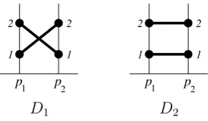
Figure 3: The two web diagrams of the web world in Example 4.
write|α|=k. LetColoursk(W) be the set ofk-colourings of web diagrams inW =W(D),
and Colours(W) =Colours1(W)∪Colours2(W)∪ · · ·.
The construction procedure that we alluded to in the Introduction happens in the following way: a `-colouring α of a web diagram D produces ` new sub-web diagrams
Dα(1), . . . , Dα(`), each of which consists of only the edges having that designated colour.
These` diagrams are not yet web diagrams, but we can relabel the heights of the vertices on each of the pegs to make them into web diagrams. Letrelbe this relabelling operation. The new web diagram D0 = Recon(D, α) = rel(Dα(1)) ⊕ · · · ⊕rel(Dα(`)) is formed by
stacking the diagrams on top of one another in increasing order of the colours. The (D1, D2) entries of the web-colouring and web-mixing matrices of W are:
M(D1W,D2) (x) = X
`>1
x`f(D1, D2, `) and R (W)
D1,D2 =
X
`>1
(−1)`−1
` f(D1, D2, `),
wheref(D1, D2, `) is the number of`-colouringsαofD1which giveRecon(D1, α) = D2. As
stated in the introduction, these web-mixing matrices occur in the calculation of scattering amplitudes in QCD. More specifically, they occur in the exponents of amplitudes, and dictate how the colour charge and kinematic degrees of freedom of highly energetic quarks and gluons are entangled by the radiation of additional lower energy gluons.
Example 4. LetD1 ={e1 = (1,2,1,2), e2 = (1,2,2,1)}. The web world generated byD1
isW(D1) = {D1, D2}whereD2 ={e01 = (1,2,1,1), e 0
2 = (1,2,2,2)}. These are illustrated
in Figure 3. There are three different colourings ofD1:
α(e1) = 1 α(e2) = 1 ⇒ Recon(D1, α) = D1
α(e1) = 1 α(e2) = 2 ⇒ Recon(D1, α) = D2
α(e1) = 2 α(e2) = 1 ⇒ Recon(D1, α) = D2
Consequently M(D1,D1W) (x) = x1 and M(W)
D1,D2(x) = 2x2. Likewise there are three different
colourings of D2:
α(e01) = 1 α(e20) = 1 ⇒ Recon(D2, α) =D2
α(e01) = 1 α(e20) = 2 ⇒ Recon(D2, α) =D2
α(e01) = 2 α(e20) = 1 ⇒ Recon(D2, α) =D2
E4
E5 E6
E1
E5
E2
E3 E4
E6
( )
P D
E
D
1 E2
[image:7.595.135.476.72.243.2]E3
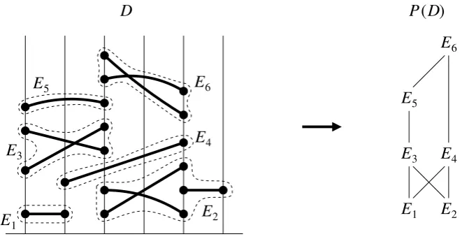
Figure 4: The decomposition poset of the web diagram in Example 6.
M(W)(x) =
x 2x2
0 x+ 2x2
and R(W)=
1 −1
0 0
.
The physical relevance of this example is that, owing to the second row of this ma-trix having no non-zero entries, only diagram D1 survives in the exponents of scattering
amplitudes. Further examples of these definitions and details can be found in [5, §2]. Every web diagramDmay be decomposed and written as a sum of indecomposable web diagrams. A poset (partially ordered set)P on the set of these constituent indecomposable web diagrams can be defined as follows:
Definition 5. LetW be a web world andD∈W. Suppose thatD=E1⊕E2⊕ · · · ⊕Ek
where each Ei is an indecomposable web diagram. Let P = {E1, . . . , Ek}. Define the
relation <1 on P ×P as follows: Ei <1 Ej if i < j and PegSet(Ei)∩PegSet(Ej) 6= ∅.
Let <2 be the transitive closure of <1 on P ×P and let be the reflexive closure of <2
onP ×P. We call P(D) = (P,) the decomposition poset of D.
Example 6. Consider the web diagram Dgiven on the left in Figure 4. The poset P(D)
we get from this diagram illustrated to its right. The constituent indecomposable web diagrams are:
E1 = {(1,2,1,1)}
E2 = {(3,5,1,3),(3,5,2,1),(5,6,2,1)}
E3 = {(1,3,1,2),(1,3,2,1)}
E4 = {(2,5,1,1)}
E5 = {(1,3,1,1)}
E6 = {(3,5,1,2),(3,5,2,1)}.
In the following sections we will repeatedly come across the Fubini polynomials (also known as theordered Bell polynomials)Fn(x) = Pnk=1k!
n k x
3
A decomposition theorem for web matrices
The main result of this section is a theorem that explains how to form the web-colouring matrix of a web world that admits a decomposition as a disjoint union of at least two other web worlds. Physical arguments tell us that such webs do not contribute to the exponents of scattering amplitudes [9] and this is something we will discuss further and exploit in Section 4.
In order to be able to state our main theorem, we must first define some new numbers and a new product on formal power series.
Let i1,...,imk ? be the number of 0-1 fillings of an m row and k column array such that there are precisely i1 ones on the top row, i2 ones in the second row, etc., and there
are no columns of only zeros.
Lemma 7. i1,...,imk
?
= [ui11ui22 · · ·uim
m] ((1 +u1)· · ·(1 +um)−1) k
.
Proof. The generating function for an entry in rowj of them×k array isu0
j+u1j = 1 +uj.
The only forbidden configuration in the array is a column of all zeros, so the generating function for columns is
m
Y
j=1
(u0j +u1j)
!
−u01u02· · ·u0m = (1 +u1)· · ·(1 +um)−1.
Since there are no restrictions on rows, the generating function for the m×k array is therefore
((1 +u1)· · ·(1 +um)−1)k.
The number of arrays with i1 ones in the first row, i2 ones in the second row, and so on,
is the coefficient of ui11ui22 · · ·uimm in the above generating function:
k i1, . . . , im
?
= [ui11ui22 · · ·uimm] ((1 +u1)· · ·(1 +um)−1)k.
It is a simple exercise to check that
k i1
?
= i1k and
k
i1,i2
?
= k−i1,k−i2,i1k +i2−k. The general expression for m= 3 is
k i1, i2, i3
?
=
k i1
i2
X
a=0
i1
a
k−i1
i2 −a
i1+i2−a
k−i3
. (1)
We will now define a new product of power series that will both help in presenting our results concerning web worlds, but also serves in establishing a new automatic way to generate general combinatorial identities from web worlds. The black diamond product
Definition 8. GivenA(1)(x), . . . , A(m)(x)∈C[[x]] whereA(k)(x) = P
n>0a (k)
n xn, we define
the black diamond product of A(1)(x), . . . , A(m)(x) as:
A(1)(x)A(2)(x) · · · A(m)(x) = X
k>0
xkX
i1>0
· · ·X
im>0
a(1)i1 · · ·a(imm)
k i1, . . . , im
? .
Let us note that if the power seriesA(i)(x) are each polynomials of degree n
i, then the
product may be written in the more computationally efficient form:
A(1)(x) · · · A(m)(x) =
n1+···+nm
X
k=0
xk X
i1∈[0,n1],...,im∈[0,nm]
i1∨···∨im6k6i1+···+im
a(1)i1 · · ·a(imm)
k i1, . . . , im
? .
(2)
The unit of the black diamond product is 1, i.e. 1A(x) =A(x). To recap on our point before the definition, due to commutativity and associativity the order in which power series appear in the black diamond product does not change its outcome. In other words, given the power series {A(i)(x)}i∈[1,m] and a permutation π∈ Sm,
A(π(1))(x)A(π(2))(x) · · · A(π(m)) =A(1)(x)A(2)(x) · · ·A(m)(x). (3)
We will abbreviate
m
z }| {
A(x)· · · A(x) to A(x)m with the convention that A(x)0 = 1.
Example 9. Suppose that A(1)(x) = · · ·=A(m)(x) = x. Then
xm =
m
z }| {
x · · · x=X
k>0
xk
k
1, . . . ,1
?
where there are mones on the right hand side. The value1,...,k1? is the number of ways to fill a table ofk columns and m rows with 0s and 1s such that there is exactly one 1 in every row and there are no columns of only 0s. This is simply another way to encode an ordered set partition of an m-set into k sets (if ais in the ith set of such a sequence then the solitary 1 in rowa of the array will be in theith column). This number is k!mk and so for all m>1,
xm =
m
X
k=1
xkk!
m
k
=Fm(x). (4)
Example 10. Using the fact thati1,i2k
?
= k−i1,k−i2,i1k +i2−k and applying Equation 2, we have
Several of the power series that arise from taking the black diamond product of simple power series expressions appear to correspond to known sequences/power series. This suggests the black diamond product may be an object worthy of study in its own right. Some examples of these include: xxn =nxn+ (n+ 1)xn+1, the coefficients in the power
series xnxn+1 appear to be given by [17, A253283], and the sequence of coefficients of
xnxn=
n
X
k=0
n+k
k
n k
xn+k
is known to count several different structures (see [17, A063007]). (We omit the proof of this final observation since it is not immediately relevant to the paper’s goal.)
We are now ready to state our main theorem.
Theorem 11. Let W1, . . . , Wm be web worlds on pairwise disjoint peg sets. Suppose that
Di, Di0 ∈Wi for alli∈[1, m]. LetW =W1∪W2∪· · ·∪Wm be a new web world which is the
disjoint union of W1, . . . , Wm. The diagrams D=D1⊕ · · · ⊕Dm andD0 =D01⊕ · · · ⊕Dm0
are web diagrams in W. Then M(D,DW)0(x)∈C[[x]] where
M(D,DW)0(x) =M (W1)
D1,D10(x) · · · M
(Wm)
Dm,D0
m(x).
Proof. Suppose that α1 is ani1-colouring of D1 which constructsD10 (i.e. Recon(D1, α) =
D01) and that α2 is a i2-colouring of D2 that constructs D02, and so on. An i-chain
is a totally ordered set of i elements. The number of ways to k-colour the diagram
D=D1⊕ · · · ⊕Dm so that it becomes D0 is the number of ways to embed the m chains
i1-chain, i2-chain, . . ., im chain, which represent the ordered colourings of D1, . . . , Dm,
respectively, into ak-chain.
The value of k must be at least the length of the largest of the m chains, and of course must be at most the sum of the lengths of all constituent m chains, i.e.
k ∈ [max(i1, . . . , im), i1 +· · · +im]. Furthermore, this embedding must be surjective,
for otherwise at least one of the k-colours {1, . . . , k} would not have any corresponding colour in the m constituent chains. One can recast this in the form of a tabular 0-1 filling problem where we have m rows and k columns whereby the column indices of the
ir ones that appear in row r of the table indicate the new colours that they take on in
the k-colouring. The surjectivity condition translates into there being no columns of all
zeros. The number of ways to do this is therefore i1,...,imk
?
.
Suppose that the entries of the web-colouring matrices that correspond to the diagrams are
M(Di,DWi)0
i(x) = a
(i)
1 x+· · ·+a (i)
nix
ni =: A(i)(x)
for all i∈ [1, m]. Since there are a(ijj) ways to colour Dj to produce D0j for allj ∈ [1, m],
the factora(1)i1 · · ·a(imm) must be included. Therefore
M(D,DW)0(x) =
n1
X
i1=1
· · ·
nm
X
im=1
a(1)i1 · · ·a(imm)
i1+···+im
X
k=i1∨···∨im
xk
k i1, . . . , im
=M(D1,DW1)0
1(x) · · · M
(Wm)
Dm,D0
m(x).
Example 12. For all i ∈ [1, m], let Di = {(2i−1,2i,1,1)} be the web diagram that
consists of a single edge between pegs 2i−1 and 2i, and let Wi be the web world that
consists of the single web diagram Di. Then M(Wi)(x) = (x), a 1×1 matrix. Since the
conditions of Theorem 11 hold, the web-colouring matrix of W ={D=D1⊕ · · · ⊕Dm},
is
M(W)(x) =
m
X
k=1
xk
k
1, . . . ,1
?!
= (Fm(x)),
from Example 9.
Corollary 13. With the same setup as in Theorem 11,
traceM(W)(x) = X
D1∈W1
· · · X
Dm∈Wm
M(D1,D1W1) (x) · · · M(Dm,DmWm) (x).
4
A method for generating combinatorial identities
In this section we will outline a method for generating combinatorial identities by using the black diamond product in conjunction with a result concerning the trace of web-mixing matrices for disjoint web worlds.
Proposition 14. Let W be a web world that is the disjoint union of at least two web
worlds. Then all entries of the web-mixing matrix R(W) are zero, and consequently
traceR(W)= 0.
A statistical physics-based proof of this result has been given in Gardi et al. [9, Section 5.1]. The essential physical idea, elaborated further in [11], is that exponents of scatter-ing amplitudes can only contain interactions between non-disjoint groups of quarks and gluons.
The relationship between the web-mixing matrices and web-colouring matrices is
R(D,DW)0 =
Z 0
−1
M(D,DW)0(x)
x dx. (5)
Integrating formal power series can be a contentious issue, so let us be clear that the integrals we perform in this paper are definite integrals and always correspond to the transformation:
a1x+a2x2+a3x3+a4x4+· · · 7→ a1 −a2/2 +a3/3−a4/4 +· · · .
Suppose that W1, . . . , Wn are web worlds on disjoint peg sets that all have the same
equivalent to one another by relabeling the peg sets that they are defined upon.) Suppose further that the diagonal entries of M are (G1(x), . . . , Gt(x)) and that
{G1(x), . . . , Gt(x)}={H1(x), . . . , Hs(x)}
where each of theHi(x) are distinct and have multiplicities (h1, . . . , hs) as diagonal entries
inM. Then
traceM(W)(x) = X
D1∈W1
· · · X
Dm∈Wm
M(D1W1,D1) (x) · · · M(Dm,DmWm) (x)
= X
(i1,...,im)∈[1,t]m
Gi1(x) · · · Gim(x)
= X
(j1,...,jm)∈[1,s]m
hj1· · ·hjmHj1(x) · · · Hjm(x)
= X
a1,...,as>0
a1+···+as=m
ha11 · · ·hass
m a1, . . . , as
H1(x)a1 · · · Hs(x)as. (6)
For the case that there are only two different power series that appear as diagonal entries of M, we have
traceM(W)(x) =
m
X
a=0
ha1hm2−a
m a
H1(x)aH2(x)m−a. (7)
Theorem 15. Let W be a web world whose web-colouring matrix has s different
diag-onal entries (H1(x), . . . , Hs(x)) that appear with multiplicities (h1, . . . , hs). Then for all
positive integers m, we have
X
a1,...,as>0
a1+···+as=m
ha11 · · ·hass
m a1, . . . , as
Z 0
−1
H1(x)a1 · · · Hs(x)as
dx x = 0.
The expression for the s= 2 case is:
m
X
a=0
ha1hm2 −a
m a
Z 0
−1
H1(x)aH2(x)m−a
dx x = 0.
We will apply the above theorem to two extremely simple web worlds to see the combinatorial identities that emerge.
Example 16. LetW be one of the web worlds of Example 12 so that M(W)(x) = (x), a
1×1 matrix. Applying Theorem 15 we haves =h1 = 1 andH1(x) =x. From Equation 4
we have
H1(x)m =
m
X
k=1
xkk!
m
and so
Z 0
−1
H1(x)m
dx x = " m X k=1 xk
k k! m k #0 −1 = m X k=1
(−1)k+1(k−1)!
m
k
.
This gives us the identity:
X
a1=m
1a1 m a1 Z 0 −1
H1(x)m
dx
x =
m
X
k=1
(−1)k+1(k−1)!
m
k
= 0. (8)
This identity can also be found in [21, Eqn. 27].
Example 17. LetW be the web world of Example 4, with
M(W)(x) =
x 2x2
0 x+ 2x2
.
In this case s= 2, H1(x) =x, H2(x) = x+ 2x2, and h1 =h2 = 1. From Equation 4,
we have H1(x)m = Fm(x). One can show that H2(x)m = F2m(x) and then applying
Theorem 15 we have
H1(x)aH2(x)m−a= 2m−a
X
k=0
xkX
i1,i2
i1!
a i1
i2!
2m−2a i2
k i1, i2
?
=
2m−a
X
k=0
xkX
i1,i2
i1!
a i1
i2!
2m−2a i2
k
k−i1, k−i2, i1+i2 −k
.
This gives us the identity
m
X
a=0 2m−a
X k=1 X i1,i2 m a
(−1)k+1
k i1!i2!
a i1
2m−2a i2
k
k−i1, k−i2, i1+i2−k
= 0. (9)
We do not know if this is a known identity.
5
Repeated entries in web matrices
results to explain some of these repetitive entries. The first theorem gives one explanation for repeated entries found on the diagonal of a web-colouring matrix, and also explains the same for the web-mixing matrix since the entries of the latter are a simple integral transformation of those in the web-colouring matrix. This theorem also builds on our earlier result [5, Thm. 3.4].
Given a posetP = (P,≺), itscomparability graph comp(P) is the graph whose vertices are the elements of P, with x, y ∈P adjacent in comp(P) if x≺y ory ≺x.
Theorem 18. Let D and D0 be web diagrams in a web world W with
D=E1⊕ · · · ⊕Ek and D0 =E10 ⊕ · · · ⊕E 0
k0,
where each of the constituent diagrams Ei and Ei0 are indecomposable. Suppose that the
members of (E1, . . . , Ek) are distinct and the members of (E10, . . . , E 0
k0) are also distinct.
If comp(P(D)) = comp(P(D0)), then MD,D(W)(x) =M(DW0,D)0(x).
Proof. First let us consider the web diagram D = E1 ⊕ · · · ⊕Ek where each of the
diagrams Ei is indecomposable. All `-colourings α such that Recon(D, α) = D must
have the property that α(e) = α(e0) whenever e, e0 ∈ Ei because Ei is indecomposable.
Thusα must be a surjective map from {E1, . . . , Ek} to [1, `]. Equivalently α surjectively
maps the k elements of the decomposition poset P(D) to the total order on [1, `]. Let us call the number of these surjective maps Θ(P(D), `). This number is related to the number Ω(P(D), `) of order preserving maps from the posetP(D) to [1, `] via an inclusion-exclusion argument:
Ω(P(D), `) =X
k
` k
(−1)`−kΩ(P(D), `).
(See [5, Lemma 3.3] for further details.) Using this we have
M(D,DW)(x) =X
`>0
Θ(P(D), `)x` =X
`>0
x`X
k
` k
Ω(P(D), k). (10)
The same is true for D0, so we have
M(DW0,D)0(x) =
X
`>0
x`X
k
` k
Ω(P(D0), k). (11)
If comp(P(D)) = comp(P(D0)) then by Stanley [18, Cor. 4.4] we have that Ω(P(D)) = Ω(P(D0)), and consequently the expressions in Equations 10 and 11 are the same.
2
1 2 3 4 5 6 7
1 1 1
2
1 3
2 1
3
1 1
3
1 2 3 4 5 6 7
1 1 1 1
2 3
2 1
1
2
1
D D0
P(D) P(D0)
[image:15.595.149.457.67.329.2]G
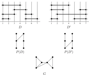
Figure 5: The web diagrams, their deconstruction posets, and web graph for Example 19.
Example 19. Let D ={(1,2,1,1),(1,3,2,1),(1,4,3,1),(3,5,2,3),(5,6,2,1),(5,7,1,1)}
and D0 = {(1,2,1,1),(1,3,2,1),(1,4,3,1),(2,7,2,3),(6,7,1,2),(5,7,1,1)}. The Hasse diagrams forP(D) andP(D0) are illustrated in Figure 5 and are clearly different. However we have that comp(P(D)) = comp(P(D0)) = G and we can conclude that M(D,DW)(x) =
M(DW0,D)0(x).
Our second result addresses general entries of the web-colouring matrix and upside-down web diagrams. Given a web diagram D, letflip(D) be the web diagram achieved by turning it upside-down. This operation is, by definition, an involution.
Definition 20. Let D = {ei = (ai, bi, ci, di) : 1 6i6m} be a web diagram in a web
world W. The flip of D, flip(D) is the web diagram inW with edges:
flip(D) ={(ai, bi, pai + 1−ci, pbi+ 1−di) : 16i6m}.
Example 21. LetDbe the web diagram in Example 19 and illustrated in Figure 5. Then
1
1 2 3 4 5 6 7
1 3
2
1 1 2 3
1 2
1
1
flip(D)
Theorem 22. LetW be a web world andD, D0 ∈W. ThenM(D,DW)0(x) =M
(W)
flip(D),flip(D0)(x).
Proof. LetW be a web world andD, D0 diagrams in W. To prove the theorem it suffices to show that for every k-colouring α of D that yields D0, there is a unique k-colouring
β of flip(D) that yields flip(D0). Define the colouring β as follows: if e = (a, b, x, y) ∈D
with α(e) = `, then let β(e) =k+ 1−`.
We will now show that Recon(flip(D), β) = flip(D0) which implies the result. Notice that in general if B1, . . . , Bm are web diagrams then
flip(B1⊕ · · · ⊕Bm) =flip(Bm)⊕ · · · ⊕flip(B1). (12)
We have:
Recon(flip(D), β) = rel(flip(D)β(1))⊕ · · · ⊕rel(flip(D)β(k))
=flip(rel(Dβ(1)))⊕ · · · ⊕flip(rel(Dβ(k))).
Using Equation 12, and applying flip to both sides of the previous equation, we have
flip(Recon(flip(D), β)) =flip(flip(rel(Dβ(1)))⊕ · · · ⊕flip(rel(Dβ(k))))
=flip(flip(rel(Dβ(k))))⊕ · · · ⊕flip(flip(rel(Dβ(1))))
=rel(Dβ(k))⊕ · · · ⊕rel(Dβ(1)).
Since those edges ofD that are coloured` using the colouring β are precisely the same as the edges that are colouredk+ 1−` using the colouringα, we haveDβ(`) = Dα(k+ 1−`)
and
flip(Recon(flip(D), β)) =rel(Dα(1))⊕ · · · ⊕rel(Dα(k))
=D0.
Applying flipto both sides gives Recon(flip(D), β) = flip(D0), as was required.
6
The squares of web-colouring and web-mixing matrices
In this section we show how to calculate the entries for the square of a web-colouring matrix and give the first mathematical proof that web-mixing matrices are idempotent. This property has been established using physical arguments by Gardi and White [12,
n Ln(x)
0 1
1 x2
2 2x3+ 2x4
3 6x4+ 12x5+ 6x6
4 x4+ 26x5+ 73x6+ 72x7+ 24x8
5 12x5+ 156x6+ 516x7 + 732x8 + 480x9+ 120x10
[image:17.595.106.493.73.191.2]6 2x5+ 126x6+ 1206x7 + 4322x8+ 7680x9+ 7320x10+ 3600x11+ 720x12
Figure 6: The first few power series Ln(x).
Theorem 23. Let W be a web world whose diagrams each have n edges. Let D, D0 ∈W
and suppose that M(D,DW)0(x) =z1x+· · ·+znxn. Then
M(W)(x)2D,D0 =
n
X
i=1
ziLi(x)
where Li(x) =
X
j,k>1
xj+k
j
X
b=0
k
X
a=0
(−1)j+k−(b+a)
j b
k a
ab
i
[image:17.595.112.397.572.705.2]. (See Figure 6.)
Figure 6 presents the expressions for Ln(x) for all n ∈ [1,7]. The previous theorem
may be summarised by saying that the square of the web-colouring matrix M(W)(x)2 is the image ofM(W)(x) under the linear operator T :
C[[x]]→C[[x]] which maps the basis
(xi)
i>0 for C[[x]] to (Li(x))i>0.
Proof. Let α ∈ Colours(W). Given two colourings α, α0 ∈ Colours(W) there is a unique
γ ∈Colours(W) such that Recon(D, γ) =Recon(Recon(D, α), β). In such an instance we write γ ≡β◦α. Recall that the (D, D0) entry of the web-colouring matrix ofW is:
M(D,DW)0(x) =
X
α∈Colours(W)
Recon(D,α)=D0
x|α|
and suppose that this is M(D,DW)0(x) =z1x+· · ·+znxn. Then
M(W)(x)2D,D0 =
X
D00∈W
M(D,DW)00(x)M (W)
D00,D0(x)
= X
D00∈W
X
α∈Colours(W)
Recon(D,α)=D00
x|α| X
β∈Colours(W)
Recon(D00,β)=D0
x|β|
=
n
X
j,k=1
X
α∈Coloursj(W) β∈Coloursk(W)
Recon(Recon(D,α),β)=D0
=
n
X
j,k=1
n
X
i=1
X
γ∈Coloursi(W)
Recon(D,γ)=D0
X
α∈Coloursj(W) β∈Coloursk(W)
γ≡β◦α
xj+k
=
n
X
i=1
X
γ∈Coloursi(W)
Recon(D,γ)=D0 n
X
j,k=1
Nj,k(i)xj+k = n
X
i=1
zi n
X
j,k=1
Nj,k(i)xj+k,
where Nj,k(i) is the number of pairs (β, α) of colourings in Coloursj(W)×Coloursk(W)
such thatβ◦αis equivalent to ai-colouringγ ∈Coloursi(W). To see how a colouring of a
colouring of a diagram can be turned into one colouring 3, we consider the ordered pairs
of colours. The diagram D is coloured withα and reconstructed to give the diagramD00. The diagramD00 is coloured with β and reconstructed to give the diagramD0.
Let us consider what happens to an edge ei = (ai, bi, xi, yi) ∈ D during this process.
In the first colouring, α(ei) = v, say, and this edge in D00 will be represented as e0i =
(ai, bi, x0i, yi0) where x0i and yi0 are the new heights of the endpoints of that edge in D00.
The edge e0i is now coloured β(e0i) = u, say, and this edge will be represented as e00i = (ai, bi, x00i, y
00
i) inD
0 wherex00
i andy
00
i are the heights of the endpoints ofe
00
i inD
0. Although
the heights change from one diagram to the next, we can still index the edge in question throughout as theith edge ei and write α(ei) = v and β(ei) =u.
Let D∈W and (α, β)∈Coloursj(W)×Coloursk(W). Let us define
Dβ,α(u, v) :={e∈D : β(e) = u and α(e) =v}.
Then
D0 =rel(Dβ,α(1,1))⊕ · · · ⊕rel(Dβ,α(1, k))⊕ · · · ⊕rel(Dβ,α(j,1))⊕ · · · ⊕rel(Dβ,α(j, k)).
In other words, the subweb-diagram of Recon(D, α) whose edges e have colour β(e) = 1 will maintain their order relative to one another in D0 and be the lowest. But amongst these edges, which will be the lowest w.r.t. the colouring α of D? It will be those edges
e ∈D that are coloured α(e) = 1, followed by all those edges e ∈D with α(e) = 2, and so on. Thus the lexicographic order on all such pairs of colourings that exists corresponds to the total order for a single colouring.
For example, if we have the pairs of colourings (β(e), α(e)) = (1,3), (1,5), (2,1), (2,2), (2,5), (3,4), then these correspond to the colours γ(e) = 1,2,3,4,5,6, respectively.
The numberNj,k(i) is therefore the number ofj×kzero-one matrices that have exactly
i ones and there are neither columns nor rows of only zeros. This number is known to be (see [3, 2] or [15, Eqn. 120]):
Nm,n(r) =
X
`>r
X
d|`
(−1)n+m−(d+`/d)
m
d
n `/d
` r
3The argument used here is reminiscent of the double application of the statistical physics-basedreplica
= m X b=0 n X a=0
(−1)n+m−(b+a)
m b n a ab r
Therefore M(W)(x)2
D,D0 =
n
X
i=1
ziLi(x) where
Li(x) =
X
j,k>1
xj+k X
a∈[0,k]
b∈[0,j]
(−1)j+k−(b+a)
j b k a ab i .
As mentioned above, the following theorem has already been proven using a physics argument (see [12, Sect. 3]). Here we give the first combinatorial proof.
Theorem 24. Let W be a web world whose web diagrams each have n edges. The
web-mixing matrix R(W) is idempotent; (R(W))2 =R(W).
Proof. Using the same method of summation as we did at the start of the proof of Theo-rem 23,
(R(W))2D,D0 =
X
D00∈W
R(D,DW)00R (W)
D00,D0
=
n
X
i,j=1
X
α∈Coloursi(W) β∈Coloursj(W)
Recon(Recon(D,α),β)=D0
(−1)i−1
i
(−1)j−1
j
=
n
X
i,j=1
(−1)i−1
i
(−1)j−1
j
X
α∈Coloursi(W) β∈Coloursj(W)
Recon(Recon(D,α),β)=D0
1.
Since
X
α∈Coloursi(W) β∈Coloursj(W)
Recon(Recon(D,α),β)=D0
1 =X
k>1
X
γ∈Coloursk(W) γ(D)=D0
X
α∈Coloursi(W) β∈Coloursj(W)
β◦α≡γ
1 =X
k>1
X
γ∈Coloursk(W) γ(D)=D0
Ni,j(k),
this gives
(R(W))2D,D0 =
n
X
i,j=1
(−1)i−1
i
(−1)j−1
j
X
k>1
X
γ∈Coloursk(W) γ(D)=D0
Ni,j(k)
=
n
X
k=1
X
γ∈Coloursk(W) γ(D)=D0
(−1)−2
n
X
i,j=1
(−1)i+j
The inner sum is
n
X
i,j=1
(−1)i+j
ij Ni,j(k) =
n
X
i,j=1
(−1)i+j
ij i X a=0 j X b=0
(−1)i+j−(a+b)
i a j b ab k = n X i,j=1 i X a=0 j X b=0
(−1)2(i+j)−(a+b)1
i i a 1 j j b ab k = n X i,j=1 i X a=0 j X b=0
(−1)a+b1
k
i−1
a−1
j−1
b−1
ab−1
k−1
= 1 k n X a,b=1
(−1)a+b
ab−1
k−1
n
X
i=a n
X
j=b
i−1
a−1
j −1
b−1
= 1 k n X a,b=1
(−1)a+b
ab−1
k−1
n a n b . (14)
We now need to prove that for 16k 6n,
F(n, k) :=
n
X
a,b=1
(−1)a+b
ab−1
k−1
n a n b
= (−1)k−1.
LetG(n, k, a) = Pn
b=1(−1)
b n b
ab−1
k−1
so thatF(n, k) =Pn
a=1(−1)
a n a
G(n, k, a). Now
ab−1
k−1
= (ab)(ab−1)· · ·(ab−k+ 1)
ab(k−1)!
= 1
(k−1)!
k X j=1 k j
(−1)k−j(ab)j−1,
the second equality comes from Graham et al. [14, eqn. (6.13)] and kj are the Stirling numbers of the first kind. Replacing this into the expression
G(n, k, a) =
n
X
b=1
(−1)b
n b
1 (k−1)!
k X j=1 k j
(−1)k−j(ab)j−1
= 1
(k−1)!
k X j=1 k j
(−1)k−jaj−1
n
X
b=1
(−1)b
n b
bj−1.
Using Graham et al. [14, Eqn. (6.19)]: m!mn = P
k m
k
kn(−1)m−k where n
m are the
Stirling numbers of the second kind. The inner sum in the previous expression is
n
X
b=1
(−1)b
n
b
bj−1 =n!
j −1
n
Since k ∈ [1, n], and j 6 k, the Stirling number on the right hand side of the previous equation will always be zero for the values that we are summing over, and the only term that will contribute will be −0j−1. This term itself will always be zero, except for when
j−1 = 0. This gives
G(n, k, a) = 1 (k−1)!
k
X
j=1
k j
(−1)k−jaj−1(−0j−1)
= 1
(k−1)!
k
1
(−1)k−1a0(−00)
= (−1)k.
Therefore F(n, k) = Pn
a=1(−1)
a n a
(−1)k = (−1)k((1−1)n−1) = (−1)k−1. This allows us to write Equation 14 as (−1)k−1/k which, in turn, means that Equation 13 is
(R(W))2D,D0 =
n
X
k=1
X
γ∈Coloursk(W) γ(D)=D0
(−1)k−1
k =R
(W)
D,D0.
7
Indecomposable permutations and a web world on two pegs
having multiple edges
In this section we consider the web world Wn whose web graph is G(Wn) = K2 and the
single edge is labelled with n. This web world consists of diagrams having two pegs and
n edges connecting the n vertices on the first peg ton vertices on the second peg. From a physics point of view, such webs have been studied for a long time [13, 7, 19]. However, they have yet to be analysed using the language of web-colouring and mixing matrices and which we will now attend to.
Every diagram D∈Wn is uniquely described as a set of 4-tuples
D={(1,2, i, πi) : π ∈ Sn}
and consequently there aren! diagrams inWn. We can abbreviate this by writingD=Dπ.
Given a permutation π =π1. . . πn and permutations α∈ S`, β ∈ Sn−`, we say that π is
the sum of the permutations αandβ ifπi =αi for alli6`and πi =`+βi−` for alli > `.
We write this as π=α+β.
If a permutationπ can be written as such a sum of smaller permutations, then we say that π is decomposable. Otherwise we say thatπ is indecomposable. LetIndn be the set
of indecomposable permutations of length n and let Ind=∪n>1Indn. Every permutation
π ∈ Sn admits a unique representation as a sum of indecomposable permutations. If
π = σ1 +· · ·+σk where every σi ∈ Ind, then Dπ = Dσ1 ⊕ · · · ⊕Dσk and we will write
Problem 25. [Word reconstruction generating function]
Given a finite wordw=w1. . . wnon a finite alphabet, letfw(k) be the number of ways to
read the word from left to right k times (each time always picking some unchosen letter) so that we arrive back at the original word w. Let Fw(x) = Pkfw(k)xk.
Example 26. Let w = cbabac = w1w2w3w4w5w6 be a word. The number of ways to
read w from left to right in one passing is 1 since we must sequentially read all letters
w1w2w3w4w5w6, so fw(1) = 1. There are several ways to read w from w in two passings:
read positions 1 through to 5 on the first passing, and read position 6 on the second passing. This is summarized by the reading vector (1,1,1,1,1,2) where j at position i
means wi is read on the jth passing. If we abbreviate this to 111112, then the other
reading vectors for k = 2 are 111122, 111222, 112222, 122222, and 122112 so fw(2) = 6.
For this case, Fw(x) = x+ 6x2+ 17x3+ 26x4 + 22x5+ 8x6.
Example 27. If all letters of a length n word w are distinct, then Fw(x) = x(1 +
x)n−1. Similarly if w is a word consisting of n copies of the same letter, then F
w(x) =
Pn
k=1k!
n k x
k =F n(x).
Theorem 28. Let Dπ ∈Wn with π =w1⊕ · · · ⊕wn where every wi ∈Ind. Let w be the
word (w1, . . . , windparts(π)) on the alphabet {w1, . . . , windparts(π)}. ThenM (W)
Dπ,Dπ(x) = Fw(x).
Proof. Let Dπ ∈ Wn with π = σ1 ⊕ · · · ⊕ σm. In order to colour the edges of Dπ so
that the same diagram is reconstructed, the colours of the edges that are in the same indecomposable part must remain the same. (Otherwise we would be constructing a web diagram which has more indecomposable parts than the original one, which would be a contradiction.) Given a set A = {a1, . . . , ai}, define σA = σa1 ⊕ · · · ⊕σai where
a1 <· · ·< ai. Let
Colourings(m, k) = {(c1, . . . , cm)∈[1, k]m : {c1, . . . , cm}= [1, k]}.
Given c∈Colourings(m, k), let Colc(i) ={j ∈[1, m] : cj =i}.
The set of colouringsc0 of edges ofDπ which results in a reconstruction of the diagram
is in 1-1 correspondence with the set of colourings c∈Colourings(m,·) such that
σ1⊕ · · · ⊕σm =σColc(1)⊕ · · · ⊕σColc(k).
This is the word reconstruction problem (Problem 25) for the word w = (σ1, . . . , σm)
which is on the alphabet {σ1, . . . , σm}.
There is no simple formula for the diagonal entries of the web-colouring matrix for this web world due to there being no ‘closed form’ answer to Problem 25. However, we have noticed some potential structure from looking at the trace of the web-colouring matrices for small values of n, outlined in Figure 7. The numbers from Figure 7 support the following conjecture for all n∈[1,8].
Conjecture 29. Leta(n) = [xn−1] trace M(W(n))(x)
. Thena(n) = (n−2)!(n2−3n+4)/2
n trace M(W(n))(x)
1 x
2 2x+ 2x2
3 6x+ 8x2+ 6x3
4 24x+ 30x2 + 42x3+ 24x4
5 120x+ 116x2+ 216x3+ 264x4+ 120x5
6 720x+ 532x2+ 1002x3+ 1920x4+ 1920x5+ 720x6
[image:23.595.114.485.71.194.2]7 5040x+ 2848x2+ 4626x3+ 11688x4+ 19200x5+ 15840x6+ 5040x7
Figure 7: The sequence of numbers that correspond to [17, A121635] (as mentioned in Conjecture 29) are the coefficients of the second highest exponent of x in each row: 2, 8, 42, 264, 1920 and 15840.
References
[1] E. Barcucci, A. Del Lungo, and R. Pinzani. “Deco” polyominoes, permutations and random generation. Theor. Comput. Sci. 159(1):29–42, 1996.
[2] P. J. Cameron, D. A. Gewurz, and F. Merola. Product action. Discrete Math.
308:386–394, 2008.
[3] P. J. Cameron, T. Prellberg, and D. Stark. Asymptotic enumeration of incidence matrices. J. Phys. Conf. Ser. 42:59–70, 2006.
[4] M. Dukes, E. Gardi, H. McAslan, D. J. Scott, and C. D. White. Webs and posets.
J. High Energy Phys. 2014(1), Article 024, 2014.
[5] M. Dukes, E. Gardi, E. Steingr´ımsson, and C. D. White. Web worlds, web-colouring matrices, and web-mixing matrices. J. Combin. Theory Ser. A 120(5):1012–1037, 2013.
[6] G. Falcioni, E. Gardi, M. Harley, L. Magnea, and C. D. White. Multiple Gluon Exchange Webs. J. High Energy Phys. 2014(10), Article 010, 2014.
[7] J. Frenkel and J. C. Taylor. Nonabelian Eikonal Exponentiation. Nucl. Phys. B
246(2): 231–245, 1984.
[8] E. Gardi. From Webs to Polylogarithms. J. High Energy Phys.2014(4), Article 044, 2014.
[9] E. Gardi, E. Laenen, G. Stavenga, and C. D. White. Webs in multiparton scattering using the replica trick. J. High Energy Phys.2010(11), Article 155, 2010.
[10] E. Gardi, J. M. Smillie, and C. D. White. On the renormalization of multiparton webs. J. High Energy Phys. 2011(9), Article 114, 2011.
[11] E. Gardi, J. M. Smillie, and C. D. White. The Non-Abelian Exponentiation theorem for multiple Wilson lines. J. High Energy Phys.2013(06), Article 088, 2013.
[13] J. G. M. Gatheral. Exponentiation of Eikonal Cross-sections in Nonabelian Gauge Theories. Phys. Lett. B 133(1&2):90–94, 1983.
[14] R. L. Graham, D. E. Knuth, and O. Patashnik.Concrete Mathematics: A Foundation for Computer Science. 2nd edition. Addison-Wesley Longman Publishing Co., 1994.
[15] M. Maia and M. Mendez. On the arithmetic product of combinatorial species. Dis-crete Math. 308(23):5407–5427, 2008.
[16] A. Mitov, G. Sterman, and I. Sung. Diagrammatic Exponentiation for Products of Wilson Lines. Phys. Rev. D 82, Article 096010, 2010.
[17] The On-Line Encyclopedia of Integer Sequences, published electronically at
http://oeis.org, 2010.
[18] R. P. Stanley. Two Poset Polytopes. Discrete Comput. Geom. 1(1):9–23, 1986.
[19] G. F. Sterman. Infrared Divergences in Perturbative QCD.AIP Conf. Proc.74:22–40, 1981.
[20] A. A. Vladimirov. Exponentiation for products of Wilson lines within the generating function approach. J. High Energy Phys. 2015(6), Article 120, 2015.
[21] Eric W. Weisstein. Stirling Number of the Second Kind. From MathWorld – A Wolfram Web Resource.
http://mathworld.wolfram.com/StirlingNumberoftheSecondKind.html


![Figure 7: The sequence of numbers that correspond to [17, A121635] (as mentioned inConjecture 29) are the coefficients of the second highest exponent of x in each row: 2, 8,42, 264, 1920 and 15840.](https://thumb-us.123doks.com/thumbv2/123dok_us/1520830.104679/23.595.114.485.71.194/figure-sequence-numbers-correspond-mentioned-inconjecture-coecients-exponent.webp)