A two-temperature open-source CFD model for hypersonic reacting flows, part two : multi-dimensional analysis

Article

A Two-Temperature Open-Source CFD Model for

Hypersonic Reacting Flows, Part Two:

Multi-Dimensional Analysis

†

Vincent Casseau1,2,_*,‡_{, Daniel E. R. Espinoza}1,2,‡_{, Thomas J. Scanlon}1,2,‡_{and Richard E. Brown}2,‡

1 _{James Weir Fluids Laboratory, University of Strathclyde, Glasgow G1 1XJ, UK;} [email protected] (D.E.R.E.); [email protected] (T.J.S.)

2 _{Centre for Future Air-Space Transportation Technology, University of Strathclyde, Glasgow G1 1XJ, UK;} [email protected]

* Correspondence: [email protected]; Tel.: +44-141-548-5040

† This paper is an extended version of our paper published in Casseau, V.; Scanlon, T.J.; John, B.; Emerson, D.R.; Brown, R.E. Hypersonic simulations using open-source CFD and DSMC solvers.

InDSMC and Related Simulations, Proceedings of the 30th International Symposium on Rarefied Gas

Dynamics, Victoria, BC, Canada, 10–15 July 2016; Ketsdever, A.; Struchtrup, H., Eds.; AIP Publishing, Melville, NY, USA; Volume 1786, 050006.

‡ These authors contributed equally to this work.

Academic Editors: Konstantinos Kontis and Mário M. G. Costa

Received: 30 September 2016; Accepted: 8 December 2016; Published:14 December 2016

Abstract:hy2Foamis a newly-coded open-source two-temperature computational fluid dynamics

(CFD) solver that has previously been validated for zero-dimensional test cases. It aims at (1) giving open-source access to a state-of-the-art hypersonic CFD solver to students and researchers; and (2) providing a foundation for a future hybrid CFD-DSMC (direct simulation Monte Carlo) code within the OpenFOAM framework. This paper focuses on the multi-dimensional verification of hy2Foamand firstly describes the different models implemented. In conjunction with employing the coupled vibration-dissociation-vibration (CVDV) chemistry–vibration model, novel use is made of the quantum-kinetic (QK) rates in a CFD solver.hy2Foamhas been shown to produce results in good agreement with previously published data for a Mach 11 nitrogen flow over a blunted cone and with thedsmcFoamcode for a Mach 20 cylinder flow for a binary reacting mixture. This latter case scenario provides a useful basis for other codes to compare against.

Keywords: hypersonics; computational fluid dynamics; two-temperature solver; OpenFOAM;

verification; direct simulation Monte Carlo

1. Introduction

The Knudsen number, defined as the ratio of the mean free path of the gas particles to the characteristic length of the problem, is commonly employed to gauge the degree of rarefaction of a gas. During the entry of a planetary atmosphere at hypervelocities, a craft will traverse the full range of the Knudsen number, from the free-molecular regime down to the continuum regime. Practically, this translates into the need for different numerical techniques to resolve the flow-field past such hypersonic bodies.

The direct simulation Monte Carlo (DSMC) method developed by Bird [1] is a particle-based methodology that is particularly well-suited for computing high Knudsen number flows, typically above 0.05, while the conventional computational fluid dynamics (CFD) approach that solves the Navier–Stokes–Fourier (NSF) equations is generally adopted for the lower range, below 0.005. In between lies an intermediate zone where DSMC is computationally prohibitive and where

conventional CFD fails due to the presence of non-continuum regions within the flow-field. To extend the range of applicability of the NSF equations towards the continuum–transition regime, Park formulated the two-temperature CFD model [2], thus distinguishing the trans-rotational energy pool from the vibro-electronic energy pools and modelling the energy exchange processes via vibrational rate equations.

Open-source solvers dedicated to the study of the hypersonic regime are very scarce. Among such codes arehy2FoamanddsmcFoam.hy2Foam[3] is a new two-temperature CFD solver developed at the University of Strathclyde [4,5] within the framework of the open-source CFD platform OpenFOAM [6]. It aims at (1) giving open-source access to a state-of-the-art hypersonic CFD solver to students and researchers; and (2) providing a foundation for a future hybrid CFD-DSMC code [7].

For rarefied gas flow environments, OpenFOAM possesses a DSMC solver calleddsmcFoam that has been developed and validated at the same University [8,9]. The two main features of dsmcFoam are that vibrational-translational post-collision energy redistribution is executed using a quantum version of the Larsen–Borgnakke procedure [8,10] and that chemical reactions are described by Quantum-Kinetic (QK) theory, as initially proposed by Bird [11].

The primary objective of this paper concerns the verification and validation of hy2Foamfor multi-dimensional case scenarios. The secondary goal is the assessment, for a two-dimensional gas flow, of one of the conclusions formulated in [5], namely that the combination of a particular chemistry–vibration model with chemical rates derived from QK theory provides a satisfactory consistency between the CFD and DSMC codes.

2. Methodology

This section essentially describes the state-of-the-art numerical procedures that have been implemented inhy2Foamto solve hypervelocity flow-fields in near-thermal equilibrium.

2.1. Non-Equilibrium Navier–Stokes–Fourier Equations

The computation of transient hypersonic reacting flows in the continuum regime traditionally employs the non-equilibrium Navier–Stokes–Fourier (NSF) equations. These are shown below in flux–divergence form using a Cartesian coordinate system for a mixture composed of Ns species,

includingNmmolecules [12]:

∂U ∂t +

∂(Fi,inv−Fi,vis)

∂xi

=W˙ . (1)

The vector of conserved quantities,U, is defined as

U = (ρ,ρs,ρu, ρv,ρw, Eve,m, E)T, s∈Ns, m∈Nm, (2)

whereu,v, andware the components of the velocity vector.ρis the mass density of the fluid andρsis

the partial density of speciess. The flux vectors are split into inviscid and viscous contributions and are written as follows:

F_i,inv= 

           

ρui

ρsui

ρuiu+δi1p

ρuiv+δi2p

ρuiw+δi3p

Eve,mui

(E+p)ui



           

F_i,vis=              0

−Js,i

τi1

τi2

τi3

−qve,i,m−eve,mJm,i

τijuj−qtr,i−qve,i−

∑

hrJr,i

             , (4)

where the indexirefers to one of the three dimensions of space andδis the Kronecker delta.EandEve,m

represent, respectively, the total energy and the total vibro-electronic energy for moleculem. In the remainder of the article, the indextrdenotes the trans-rotational energy mode,vethe vibro-electronic energy mode andethe electron energy mode.hsis the enthalpy per unit mass of speciess, while the

pressure,p, is recovered from the partial pressures using Dalton’s law

p=

∑

s6=e

ps+pe=

∑

(ρsRsTtr) +ρeReTve,ref, (5)

whereRs is the specific gas constant. Finally, the electron temperature is set to the vibro-electronic

temperature of a reference particle,Tve,ref.

In Equation (4),τijrepresent the components of the viscous stress tensor, which can be written

as follows:

τij =µ ∂ui ∂xj

+∂uj

∂xi

!

+ (λ+µb)

∂uk

∂xk

δij, (6)

whereµis the shear viscosity,λis the second viscosity coefficient, andµ_bis the bulk viscosity. This

work assumes that Stokes’ hypothesis is valid, namely thatµb = 0 and that the shear and second

viscosity are not independent quantities but given by the relationλ=−2₃µ. Inhy2Foam, the species

shear viscosities can be considered as temperature-independent, or either set to follow Blottner’s formula [13] or a power law. The spatial components of the heat conduction vector are assumed to follow Fourier’s law

qtr,i=

∑

qtr,i,s =

∑

−κtr,s

∂Ttr

∂xi

fors∈Ns\ {e} (7)

and

qve,i =

∑

qve,i,s=

∑

−κve,s ∂Tve,s

∂xi for

s∈Ns. (8)

The thermal diffusivitiesκtr,s andκve,s can be considered as temperature-independent, or set

to follow Eucken’s formula [12,14]. Mixture quantities are recovered from species quantities using a mixing rule. The Wilke [15], Gupta [16], and Armaly and Sutton [17] mixing rules have been implemented, and the latter one is being used in this work, as recommended in the review of Palmer and Wright [18].

The diffusion fluxes,Js,i, are governed by Fick’s law with a correction term to ensure mass

conservation [19]

Js,i = Is,i−Ys

∑

Ir,i, fors,r∈Ns\ {e},

= Me

∑

Cr× Jr,i

Mr otherwise,

with

Is,i =−ρDs

∂Ys

∂xi

, (10)

whereYis the mass-fraction and with the effective diffusion coefficient of speciessin the mixture defined as [20]

Ds = (1−Xs)

∑

r6=s

Xr Ds,r

!−1

fors,r∈ Ns\ {e}, (11)

in whichXis the molar-fraction,C_r represents the charge of speciesrandMis the molecular weight. The binary diffusion coefficients,Ds,r, are modelled using binary collision integrals∆s,ras [21]

Ds,r= kBTtr

p∆s,r. (12)

Finally, the source term vector,W˙ , is written as

˙

W =0, ˙ωs, 0, 0, 0, ˙ωv,m, 0

T

, (13)

where ˙ωsis the net mass production of speciessand ˙ωv,m, form∈Nm, is defined as follows:

˙

ωv,m = Qm,V−T+Qm,V−V +Qm,C−V+Qm,e−V, if the reference molecule foreis notm, = Qm,V−T+Qm,V−V +Qm,C−V+Qm,e−V +Qh−e+Qe−i+U· ∇pe otherwise,

(14)

whereUrepresents the velocity vector. The meaning of the different vibrational source terms that appear in Equation (14) is given in the subsequent paragraphs.

2.2. Energy Transfers

The decomposition of the total energy, E, as shown in Equation (15), allows the isolation of different energy pools, each of them being described by a specific temperature and exchanging energy with the other pools:

E = 1

2ρ

∑

i +

∑

s6=e

Et,s +

∑

s6=e

Er,s +

∑

s6=e

Ev,s +

∑

s6=e

Eel,s + Ee +

∑

s6=e

ρsh◦_{s . (15)}

In order of appearance in Equation (15) are the kinetic, translational (index t), rotational (r), vibrational (v), electronic (el), electron (e), and chemical energies.uiare the spatial components of the

velocity vector andh◦s is the standard enthalpy of formation of speciess. The relationship between the

total energy of a specific mode and the energy per unit mass of speciessis given in Equation (16) for the electronic energy mode

Eel=

∑

Eel,s =

∑

ρseel,s (16)

and the different energies per unit mass of species are detailed below for each mode:

et= 3

2RsTtr, (17)

ev,s =Rs θv,s

expθv,s

Tve,s

−1

, (19)

ee =ReTve,ref, (20)

eel,s=Rs

∞

∑

gi,sθel,i,sexp(−θel,i,s/Tve,s)

∞

∑

gi,sexp(−θel,i,s/Tve,s)

. (21)

The simple harmonic oscillator model [11] is utilized for the vibrational mode, withθv,sbeing the

characteristic vibrational temperature for speciess. θel,i,s and gi,s are the characteristic electronic

temperature and the degeneracy degree of a given electronic state i for species s, respectively. The two-temperature model formulation adopted inhy2Foamthen consists in rewriting Equation (15) as follows:

E = 1

2ρ

∑

2

i + Etr +

∑

s6=e

Eve,s + Ee +

∑

ρsh

◦

s (22)

with

Etr =Et+Er (23)

and

Eve,s =Ev,s+Eel,s. (24)

The vibrational source terms introduced into the NSF equations in the preceding paragraph are now described in sequence. The energy exchange between the trans-rotational and the vibro–electronic energy modes (V–T), designated byQm,V−T, is dictated by the Landau–Teller equation [22] and may be written as

Qm,V−T =ρm

∂eve,m(Tve,m)

∂t =ρm

eve,m(Ttr)−eve,m(Tve,m)

τm,V−T

m∈Nm, (25)

whereτm,V−T is the molar-averaged V–T relaxation time. This former quantity is evaluated as the summation of the Millikan and White semi-empirical correlation [23] and Park’s correction factor [2], and later denoted as MWP. It becomes

τm,V−T =

∑

Xs

∑

Xs/τm−s,V−T

m∈ Nm, (26)

whereXis the species molar-fraction andτm−s,V−T is the interspecies relaxation time expressed as

τm−s,V−T = 1 pexp

h Am,s

T_tr−1/3−Bm,s

−18.42i+ 1 ¯

cmσv,mnm,s with pin atm. (27)

For a given colliding pair (m,s), the tabulated values ofAm,sandBm,sused in this paper can be

found in [4]. The collision-limited relaxation time introduced by Park [2] is a function of the average molecular speed, ¯cm, the limited collision cross-section,σv,m, and the number density of the colliding

The second V–T model tested in this work is the SSH theory named after Schwartz, Slawsky, and Herzfeld [24]. The coefficients of this latter model are taken from the work of Thivet [25] and a blended model is created with the MWP formulation for molecule-atom collisions.

Vibrational–vibrational (V–V) energy transfer is denoted byQm,V−V and modelled according to the formulation given by Knab et al. [26,27], as described in [4]. In Equation (14),Qh−e,Qm,e−V, andQe−i stand for the energy exchange between free-electrons and heavy-particles, free-electrons and the vibrational mode, and the vibrational energy removal due to electron impact ionisation, respectively. They are assumed to be zero in this work. The term inU· ∇perepresents an approximation to the

work done on the electrons by the electric field induced by the electron pressure gradient [28]. Finally, the vibro-electronic energy added or removed by chemical reactions to speciesm, and represented by Qm,C−V, is modelled either with the Park TTv model [2] or the coupled vibration-dissociation-vibration (CVDV) model inhy2Foam[4].

2.3. Departure from the Continuum Regime

The local gradient-length Knudsen number introduced by Boyd [29] is often used as a breakdown parameter in the literature (e.g., in [30–33]). For a local macroscopic flow quantityφ, it is written as

KnGLL−φ=

λ

φ|∇φ|, (28)

whereλ is the local mean free path of the gas molecules andφcan either be the gas density, the

temperature, or the magnitude of the velocity vector|U|(ormax(|U|,a)in the denominator, wherea is the speed of sound for low-speed regions [34]). The degree of local continuum breakdown is then evaluated as the maximum for all of the aforementioned flow quantities

KnGLL =max

KnGLL−ρ,KnGLL−Ttr,KnGLL−Tve,KnGLL−|U|

, (29)

and the regions where the continuum assumption does not hold are identified whenKnGLLexceeds

a given breakdown value,KnBr, typically being taken equal to 0.05. This parameter is key in hybrid

CFD-DSMC codes.

3. Results and Discussion

3.1. Mach 11.3 Blunted Cone

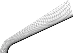
In this section, a non-reacting nitrogen flow past a blunted cone is examined at Mach 11.3. The case is composed of a 6.35 mm-radius nose followed by a flat plate forming a 25◦angle with the free-stream flow direction and whose streamwise extension is 5 cm. The 2D axisymmetric mesh that has been employed is shown in Figure1. The structured grid is aligned with the bow shock and consists of 600 by 200 cells. The first spacing at the wall surface is set to 2µm by default and to 10µm for comparison purposes.

The initial conditions of this case scenario are given in Table 1. The free-stream velocity corresponding to a Mach number of 11.3 is 2764.5 m/s. The free-stream temperature and pressure are 144.4 K and 21.9 Pa, respectively. The wall is assumed to be isothermally heated to a temperature of 297.2 K. This simulation uses the MWP formulation for V–T energy exchange and the Blottner and Eucken formulas to compute transport properties. The variable hard sphere model is chosen for the calculation of the mean-free-path and the Knudsen number is computed using the streamwise extent of the cone as the characteristic length. The non-equilibrium boundary conditions employed at the cone surface are the first-order Smoluchowski temperature jump [35] and Maxwell velocity slip [36], with the accommodation coefficients being taken as equal to unity. The set-up for this case can be found in the Supplementary Materials.

The hy2Foam solver uses the numerics present in the official OpenFOAM application rhoCentralFoam[37], namely the KNP central-upwind schemes of Kurganov, Noelle and Petrova [38]. Hence,hy2Foamis first order accurate in time and second order accurate in space. Improving the numerics of the solver to better capture the near-wall region notably is an ongoing area of research. Convergence was achieved after 2.8 h of computations on the ARCHIE-WeSt (Academic and Research Computer Hosting Industry Enterprise in the West of Scotland) High Performance Computer [39]. The run used 24 Intel Xeon X5650 2.66 GHz cores (Santa Clara, CA, USA) with 48 GB RAM and 4xQDR Infiniband Interconnect computer-networking communications.

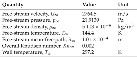
Table 1.Initial conditions for the Mach 11.3 blunted cone.

Quantity Value Unit

Free-stream velocity,U_∞ 2764.5 m/s Free-stream pressure,p_∞ 21.9139 Pa Free-stream density,ρ∞ 5.113×10−4 kg/m3 Free-stream temperature,T_∞ 144.4 K Free-stream mean-free-path,λ_∞ 1.01×10−4 m

Overall Knudsen number,Knov 0.002

-Wall temperature,Tw 297.2 K

This particular configuration has already been studied by Wang and Boyd [40], using the MONACO DSMC code and a Navier–Stokes CFD solver from the University of Michigan. The results from these simulations are reported in the subsequent graphs with the denominationDSMC: MONACO andCFD: Michigan. Moreover, experimental data is also shown in Figure2d,f and correspond to the run 31 of the CUBRC (CUBRC Inc., Buffalo, NY, USA) experiments [41].

The emphasis is placed on stagnation line data and then on surface properties such as the pressure coefficient,Cp, friction coefficient,Cf, and Stanton number,St, respectively, given by

Cp= p−p∞

0.5ρ∞U2

∞, (30)

C_f = τ

0.5ρ_∞U_∞2 , (31)

St= q

0.5ρ_∞U3_∞, (32)

those essential aerothermodynamic quantities being shown in Figure2d–f.

by the use of a different viscosity model (the power law was used in [40]). As it is the case in most simulations of hypersonic flow-fields, the bow shock thickness given by the NSF equations is clearly under-predicted, as shown by the different DSMC profiles.

Normalised temperature,

T

/

T∞

Stagnation line position [mm] non-reacting N2

DSMC: MONACO CFD: Michigan hy2Foam 0 5 10 15 20 25 30 35

-3 -2 -1 0

Ttr

Tt Tv, N2 Normalised density,

ρ

/

ρ∞

Stagnation line position [mm] non-reacting N2

DSMC: MONACO CFD: Michigan hy2Foam 0 5 10 15

-2 -1 0

(a) (b)

Normalised velocity,

U

/

U∞

Stagnation line position [mm] non-reacting N2

DSMC: MONACO CFD: Michigan hy2Foam 0 0.25 0.5 0.75 1

-2 -1 0

Pressure coefficient

Axial distance from stagnation point [cm]

non-reacting N₂

Experiments DSMC: MONACO CFD: Michigan hy2Foam 0 0.5 1

0 1 2 3 4

(c) (d)

Friction coefficient

Axial distance from stagnation point [cm]

non-reacting N2

DSMC: MONACO CFD: Michigan

hy2Foam, ∆x, 0 = 2 µm

∆x, 0 = 10 µm

0 0.05 0.1 0.15

0 1 2 3 4

Stanton number

Axial distance from stagnation point [cm]

non-reacting N₂

Experiments DSMC: MONACO CFD: Michigan

hy2Foam, ∆x, 0 = 2 µm

∆x, 0 = 10 µm

0 0.1 0.2

0 1 2 3 4

(e) (f)

Figure 2. (a–c) Stagnation line profiles, and (d–f) surface quantities along the blunted cone; (a) normalised temperature; (b) normalised mass density; (c) normalised velocity; (d) pressure coefficient; (e) friction coefficient; (f) Stanton number.

The variable hard sphere mean-free-path computed byhy2Foamin the wall vicinity is of the order of 2µm. Good DSMC practice dictates that the mean-free-path to cell-size ratio should exceed one so one could argue that the DSMC mesh employed might not be fine enough near the wall to accurately capture the surface aerothermodynamic coefficients along the body, e.g., the peak amplitude of the skin-friction.

Finally, this case is a good illustration that a hypersonic simulation can now be carried out using open-source packages all the way from pre- to post-processing using Gmsh (version 2.11.0) [42] as a mesher,hy2Foamas a solver, Paraview [43] (version 4.1.0, Sandia Corporation, Albuquerque, NM, USA and Kitware Inc., Clifton Park, NY, USA) as a visualization utility, and Gnuplot [44] (version 5.0) as a grapher.

3.2. Mach 20 Cylinder

This section focuses on the hypersonic Mach 20 flow of nitrogen over a two-dimensional circular cylinder of radiusR= 1 m. A symmetry plane exists about they=0 plane allowing the modelling solely of the upper half of the domain to be considered. The streamwise extent of the computational domain spans from−1.8 m to 5 m and the initial conditions are listed in Table2.

A free-stream velocity of 6047 m·s−1 is applied with a free-stream pressure of 0.89 Pa and temperatureT∞= 220 K. Such a temperature is high enough to result in a vibrationally-excited and chemically active flow-field. The cylinder wall is held at a uniform temperature of 1000 K. The overall Knudsen number of 0.0022 lies in the lower range of the continuum-transition regime; however, the gas locally may lie in the transition regime.

Table 2.Initial conditions for the Mach 20 cylinder.

Quantity Value Unit

Free-stream velocity,U_∞ 6047 m/s Free-stream pressure,p∞ 0.89 Pa Free-stream density,ρ∞ 1.363×10−5 kg/m3 Free-stream temperature,T_∞ 220 K Free-stream mean-free-path,λ_∞ 4.45×10−3 m

Overall Knudsen number,Knov 0.0022

-Wall temperature,Tw 1000 K

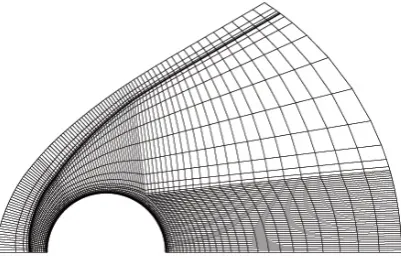
The mesh used in this investigation is shown in Figure3and was constructed using Ansys ICEM (Integrated Computer Engineering and Manufacturing) CFD (Canonsburg, PA, USA) [45]. This mesh consists of 155,000 cells with the first cell spacing at the cylinder wall set to 2 microns. Both Maxwellian velocity slip and Smoluchowski temperature jump boundary conditions were applied at the walls with the accommodation coefficient equal to 1.

For the shear viscosity and the thermal conductivity, the Blottner and Eucken formulae were applied, respectively, while the mixing rule employed was that of Armaly and Sutton. Both MWP and SSH formulations are successively used for V–T energy transfer for comparison purposes. The different set-ups are summarised in Table3together with a run identification number.

Table 3.Computational fluid dynamics (CFD) simulations performed.

Run Number V–T Transfer Electronic Mode CV Model Rates

1 MWP no CVDV QK

2 SSH no CVDV QK

3 MWP no Park TTv Park

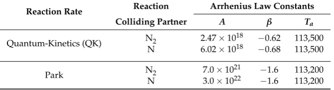
Two chemical reactions were also considered, these being the irreversible molecule–molecule and molecule–atom dissociation of nitrogen

N₂ + N₂ −−→ 2 N + N₂, N₂ + N −−→ 2 N + N.

The Arrhenius rate constants are shown in Table4in which the units ofAandTaare given in

m3·mol−1·s−1and Kelvin, respectively. They are derived from the QK theory [8] and Park’s rates for use in a two-temperature CFD solver [2].

Finally, two configurations associating a chemistry–vibration model with a set of chemical rates have been studied. The first one is called CVDV-QK and has been tested for zero-dimensional heat bath scenarios only [4]. The second configuration, subsequently named Park, is the one conventionally used in hypersonics and combines the Park TTv model with Park’s rates. The set-up for this case can be found in the Supplementary Materials.

Table 4.Parameters for the evaluation of the forward rate constant.

Reaction Rate Reaction Arrhenius Law Constants

Colliding Partner A β Ta

Quantum-Kinetics (QK) N2 2.47×1018 −0.62 113,500 N 6.02×1018 −0.68 113,500

Park N2 7.0×1021 −1.6 113,200

N 3.0×1022 −1.6 113,200

The DSMC configuration is provided in [5], and good DSMC practice was satisfied for both the mesh and time-step. In the DSMC mesh, a total of 5.5 million cells were employed, which were filled with over 80 million equivalent DSMC particles at steady-state. Non-reacting case scenarios were also executed in [5], and the analysis will not be repeated here, although some of the results will be reported in the following graphs and tables.

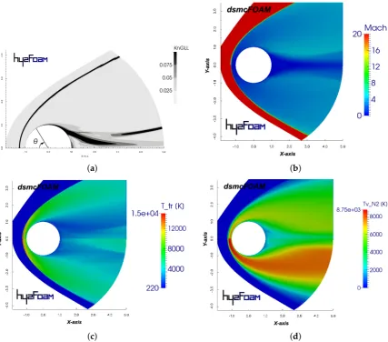
The departure from local thermodynamic equilibrium is shown in Figure4a for the CFD run number 2 using the local gradient-length Knudsen number. Dark grey and black colours indicate KnGLLvalues beyond 0.05 and cover, as expected, the bow shock and the near-wake areas. Similar

results were found for the other runs.

The Mach and trans-rotational temperature fields given byhy2FoamanddsmcFoamin Figure4b,c compare well in the compression region, forx<0. In the wake of the cylinder, however,Ttris generally

Larsen–Borgnakke method indsmcFoam, which promotes a quicker energy harmonisation in expansion regions (whereTv>Ttr) as reported in [4] using a zero-dimensional analysis. The Park combination

used in run 1 is the instance that provides less accurate results with local vibrational temperatures above 10,000 K.

(a) (b)

(c) (d)

Figure 4. Computational fluid dynamics-direct simulation Monte Carlo (CFD-DSMC) flow-field comparisons for run number 2. In (b–d): thedsmcFoamsolution is represented in the upper half and

thehy2Foamsolution in the lower half. (a) Local gradient-length Knudsen number; (b) Mach number;

(c) trans-rotational temperature; and (d) vibrational temperature.

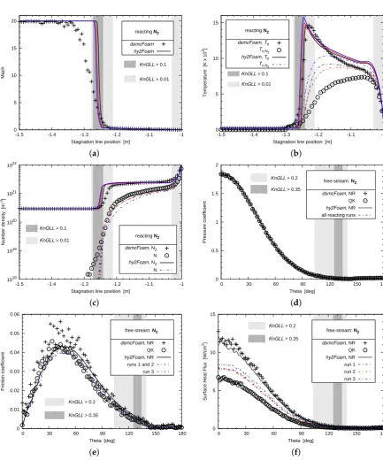
Figure5a–c compares the stagnation line profiles of Mach number, temperature, and number density given byhy2FoamanddsmcFoam. It is normally evident that the bow shock is more diffuse when using the DSMC method compared with CFD. However, it is evident that the shock stand-off distances are almost identical using both solvers and are approximately equal to 0.25 m, which is about 5 cm closer to the body than for the non-reacting case [5]. The peak in trans-rotational temperature is correctly determined using the CVDV-QK combination for both runs 1 and 2 and is slightly over-predicted using the Park combination. As shown previously in Figure4d, the trend in vibrational temperature shows a steeper increase across the shock wave. In Figure5c, the evolution of the species number densities for all runs is in satisfactory agreement withdsmcFoamoutside of the KnGLL >0.01 band. The early production of atomic nitrogen within the shock is not captured in the

Surface properties of pressure coefficient, skin friction and heat transfer are shown in Figure5d–f for both non-reacting (NR) and reacting simulations. There is a reasonable agreement between the CFD and DSMC solvers forCpandCf.

Mach

Stagnation line position [m] reacting N2

dsmcFoam hy2Foam 0 5 10 15 20

-1.5 -1.4 -1.3 -1.2 -1.1 -1

KnGLL > 0.1

KnGLL > 0.01

Temperature [K x 10

3]

Stagnation line position [m] reacting N2

dsmcFoam, Ttr

Tv,N2

hy2Foam, Ttr

Tv,N2

0 5 10 15

-1.5 -1.4 -1.3 -1.2 -1.1 -1

KnGLL > 0.01

KnGLL > 0.1

(a) (b)

Number density [m

-3]

Stagnation line position [m] reacting N2

dsmcFoam, N2

N

hy2Foam, N2

N 1018 1019 1020 1021 1022

-1.5 -1.4 -1.3 -1.2 -1.1 -1

KnGLL > 0.1

KnGLL > 0.01 Pressure coefficient

Theta [deg]

free-stream: N2

dsmcFoam, NR

QK

hy2Foam, NR

all reacting runs

0 0.5 1 1.5 2

0 30 60 90 120 150 180

KnGLL > 0.2

KnGLL > 0.35

(c) (d)

Friction coefficient

Theta [deg]

free-stream: N2

dsmcFoam, NR

QK

hy2Foam, NR

runs 1 and 2 run 3 0 0.01 0.02 0.03 0.04 0.05 0.06

0 30 60 90 120 150 180

KnGLL > 0.2

KnGLL > 0.35

Surface Heat Flux [W/cm

2]

Theta [deg]

free-stream: N2

dsmcFoam, NR

QK

hy2Foam, NR

run 1 run 2 run 3 0 5 10 15

0 30 60 90 120 150 180

KnGLL > 0.2

KnGLL > 0.35

(e) (f)

Figure 5. (a–c): Stagnation line profiles. CFD run 1:blacklines, run 2:redlines, run 3:bluelines. (d–f): surface quantities around the cylinder. (a) Mach number; (b) temperature; (c) number density; (d) pressure coefficient; (e) skin-friction coefficient; (f) surface heat flux.

CH, is however showing larger discrepancies between the two codes. There are several factors that

could explain this observation: (1) aKnGLLnumber greater than 0.1 all around the cylinder; (2) a

different treatment of the vibration-translational energy transfer between CFD and DSMC codes; and (3) the use of the KNP numerical schemes inhy2Foamthat are known for being too dissipative in the near-wall region. It is also shown that the CVDV-QK association is producing a 27% larger integrated heat flux as compared withdsmcFoam, while the Park combination overpredictsCHby 39%.

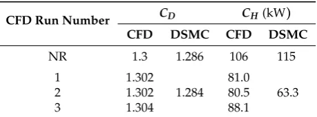
Table 5.Aerothermodynamic coefficients.

CFD Run Number CD CH(kW) CFD DSMC CFD DSMC

NR 1.3 1.286 106 115

1 1.302

1.284

81.0

63.3

2 1.302 80.5

3 1.304 88.1

CDis the drag coefficient andCHrepresents the integrated heat flux.

4. Conclusions

The newly-coded open-source two-temperature CFD solver hy2Foam has been extended to simulate hypersonic multi-dimensional case scenarios.hy2Foamhas shown to perform as well as a Navier–Stokes CFD solver from the University of Michigan for a Mach 11 blunted cone, and to be in satisfactory agreement with thedsmcFoamcode for a Mach 20 flow of a binary reacting mixture around a circular cylinder. For this latter case, the aerothermodynamic loads were better estimated using the novel CVDV-QK model combination rather than the conventional Park combination, when compared to thedsmcFoamcode. This result reaffirms the predictions found using zero-dimensional cases in [4]. Finally, it is considered that the cylinder case scenario presented in this paper provides a useful basis for other codes to compare against.

Future work for the extension ofhy2Foamwill include the development of an 11-species plasma model for application in weakly-ionized flow environments. The discrepancies observed between the CFD and DSMC codes forKnGLL numbers outwith the continuum regime will motivate the

development of an open-source hypersonic hybrid hydrodynamic-molecular gas flow solver using both thedsmcFoamandhy2Foamcodes [7].

Supplementary Materials:The following are available online at www.mdpi.com/2226-4310/3/4/45/s1.

Acknowledgments: Vincent Casseau wishes to thank the James Weir Fluids Laboratory (University of Strathclyde, Glasgow, UK) and the centre for Future Air-Space Transportation Technology (cFASTT) (University of Strathclyde, Glasgow, UK) who supported this work. Vincent Casseau would also like to thank Benzi John and David R. Emerson from the Science and Technology Facilities Council (STFC) Daresbury Laboratory in Warrington, UK for setting-up and running the DSMC computations and acknowledge Jimmy-John Hoste from cFASTT for his help in testing thehy2Foamsolver. The CFD results were obtained using the Engineering and Physical Sciences Research Council (EPSRC) funded ARCHIE-WeSt High Performance Computer (www.archie-west.ac.uk/). EPSRC grant no. EP/K000586/1.

Author Contributions: Vincent Casseau implemented the hy2Foam solver; Vincent Casseau and Daniel E. R. Espinoza performed the computations; Vincent Casseau, Daniel E. R. Espinoza, Thomas J. Scanlon and Richard E. Brown analyzed the data; and Vincent Casseau and Thomas J. Scanlon wrote the paper.

Conflicts of Interest:The authors declare no conflict of interest.

References

1. Bird, G.A.Molecular Gas Dynamics and the Direct Simulation of Gas Flows; Clarendon: Oxford, UK, 1994. 2. Park, C.Nonequilibrium Hypersonic Aerothermodynamics; Wiley International: New York, NY, USA, 1990. 3. Github Repository of thehy2FoamSolver. Version 0.01, Commit 98032f1. Available online: https://github.

4. Casseau, V.; Palharini, R.C.; Scanlon, T.J.; Brown, R.E. A Two-Temperature Open-Source CFD Model for Hypersonic Reacting Flows, Part One: Zero-dimensional Analysis. Aerospace2016,3, 34.

5. Casseau, V.; Scanlon, T.J.; John, B.; Emerson, D.R.; Brown, R.E. Hypersonic Simulations using Open-Source CFD and DSMC Solvers. In Proceedings of the AIP Conference, Victoria, BC, Canada, 10–15 July 2016; Volume 1786.

6. OpenFOAM Official Website. Available online: http://www.openfoam.org/ (accessed on 2 August 2016). 7. Espinoza, D.E.R.; Casseau, V.; Scanlon, T.J.; Brown, R.E. An Open Source Hybrid CFD-DSMC Solver for High-Speed Flows. In Proceedings of the AIP Conference, Victoria, BC, Canada, 10–15 July 2016; Volume 1786.

8. Scanlon, T.J.; White, C.; Borg, M.K.; Palharini, R.C.; Farbar, E.; Boyd, I.D.; Reese, J.M.; Brown, R.E. Open source Direct Simulation Monte Carlo (DSMC) Chemistry Modelling for Hypersonic Flows. AIAA J.

2015,53, 1670–1680.

9. Palharini, R.C. Atmospheric Reentry Modelling Using an Open-Source DSMC Code. Ph.D. Thesis, University of Strathclyde, Glasgow, UK, 2014.

10. Borgnakke, C.; Larsen, P.S. Statistical collision model for simulating polyatomic gas with restricted energy exchange. InRarefied Gas Dynamics; DFVLR Press: Porz-Wahn, Germany, 1974; Volume 1, p. A7.

11. Bird, G.A. The DSMC Method, 2nd ed.; CreateSpace Independent Publishing Platform: Seattle, WA, USA, 2013.

12. Candler, G.V.; Nompelis, I. Computational Fluid Dynamics for Atmospheric Entry. InNon-Equilibrium

Dynamics: From Physical Models to Hypersonic Flights. The von Karman Institute for Fluid Dynamics:

Rhode-Saint-Genèse, Belgium, 2009.

13. Blottner, F.G.; Johnson, M.; Ellis, M.Chemically Reacting Viscous Flow Program for Multicomponent Gas Mixtures; Report No. SC-RR-70-754; Sandia Laboratories: Albuquerque, NM, USA, 1971.

14. Vincenti, W.G.; Kruger, C.H.Introduction to Physical Gas Dynamics; Krieger Publishing Company: Malabar, FL, USA, 1965.

15. Wilke, C.R. A Viscosity Equation for Gas Mixtures. J. Chem. Phys.1950,18, 517–519.

16. Gupta, R.; Yos, J.M.; Thompson, R.A.; Lee, K.P.A Review of Reaction Rates and Thermodynamic and Transport Properties for an 11-Species Air Model for Chemical and Thermal Nonequilbrium Calculations to 30,000 K; NASA RP-1232; NASA: Washington, DC, USA, 1990.

17. Armaly, B.F.; Sutton, L. Viscosity of Multicomponent Partially Ionized Gas Mixtures. In Proceedings of the 15th Thermophysics Conference, Snowmass, CO, USA, 14–16 July 1980; AIAA Paper 80-1495.

18. Palmer, G.E.; Wright, M.J. Comparison of Methods to Compute High-Temperature Gas Viscosity.

J. Thermophys. Heat Transf.2003,17, 232–239.

19. Sutton, K.; Gnoffo, P.A. Multi-Component Diffusion with Application to Computational Aerothermodynamics. In Proceedings of the 7th AIAA/ASME Joint Thermophysics and Heat Transfer Conference, Albuquerque, NM, USA, 15–18 June 1998; AIAA Paper 98-2575.

20. Hirschfelder, J.O.; Curtiss, C.; Bird, R.B. Molecular Theory of Gases and Liquids; John Wiley & Sons, Inc.: Hoboken, NJ, USA, 1954.

21. Alkandry, H.; Boyd, I.D.; Martin, A. Comparaison of Models for Mixture Transport Properties for Numerical Simulations of Ablative Heat-Shields. In Proceedings of the 51st AIAA Aerospace Sciences Meeting including the New Horizons Forum and Aerospace Exposition Grapevine (Dallas/Ft. Worth Region), Grapevine, TX, USA, 7–10 January 2013; AIAA Paper 2013-0303.

22. Landau, L.; Teller, E. On the theory of sound dispersion.Phys. Z. Sowjetunion1936,10, 34.

23. Millikan, R.C.; White, D.R. Systematics of Vibrational Relaxation. J. Chem. Phys.1963,39, 3209–3213. 24. Schwartz, R.N.; Slawsky, Z.I.; Herzfeld, K.F. Calculation of Vibrational Relaxation Times in Gases.

J. Chem. Phys.1952,20, 1591–1599.

25. Thivet, F.; Perrin, M.Y.; Candel, S. A unified nonequilibrium model for hypersonic flows. Phys. Fluids1991,

3, 2799–2812.

26. Knab, O.; Frühauf, H.H.; Jonas, S. Multiple Temperature Descriptions of Reaction Rate Constants with Regard to Consistent Chemical-Vibrational Coupling. In Proceedings of the 27th Thermophysics Conference, Nashville, TN, USA, 6–8 July 1992; AIAA Paper 92-2947.

28. Gnoffo, P.A.; Gupta, R.; Shinn, J.L. Conservation Equations and Physical Models for Hypersonic Air Flows in

Thermal and Chemical Nonequilibrium; Technical Report NASA-TP-2867; NASA Langley: Hampton, VA,

USA, 1989.

29. Boyd, I.D.; Chen, G.; Candler, G.V. Predicting failure of the continuum fluid equations in transitional hypersonic flows. Phys. Fluids1995,7, 210–219.

30. Schwartzentruber, T.E.; Scalabrin, L.C.; Boyd, I.D. A modular particle-continuum numerical method for hypersonic non-equilibrium gas flows.J. Comput. Phys.2007,225, 1159–1174.

31. Abbate, G.; Thijsse, B.J.; Kleijn, C.R. Computational Science—ICCS 2007. Part I, Chapter Coupled Navier–Stokes/DSMC Method for Transient and Steady-State Gas Flows. In Proceedings of the 7th International Conference, Beijing, China, 27–30 May 2007; Springer: Berlin/Heidelberg, Germany, 2007; Volume 225, pp. 842–849.

32. Darbandi, M.; Roohi, E. Applying a hybrid DSMC/Navier–Stokes frame to explore the effect of splitter catalyst plates in micro/nanopropulsion systems. Sens. Actuators A2013,189, 409–419.

33. Roveda, R.; Goldstein, D.B.; Varghese, P.L. Hybrid Euler/particle approach for continuum/rarefied flows.

J. Spacecr. Rocket.1998,35, 258–265.

34. Schwartzentruber, T.E.; Scalabrin, L.C.; Boyd, I.D. Hybrid Particle-Continuum Simulations of Nonequilibrium Hypersonic Blunt-Body Flowfields. J. Thermodyn. Heat Transf.2008,22, 29–37.

35. Von Smoluchowski, M. Über wärmeleitung in verdünnten Gasen.Ann. Phys. Chem.1898,64, 101–130. 36. Maxwell, J.C. On stresses in Rarefied Gases Arising from Inequalities of Temperature. Phil. Trans. R.

Soc. Lond.1879,170, 231–256.

37. Greenshields, C.J.; Weller, H.G.; Gasparini, L.; Reese, J.M. Implementation of semi-discrete, non-staggered central schemes in a collocated, polyhedral, finite volume framework, for high-speed viscous flows. Int. J. Numer. Methods Fluids2010,63, 1–21.

38. Kurganov, A.; Noelle, S.; Petrova, G. Semi-discrete central-upwind schemes for hypersonic conservation laws and Hamilton-Jacobi equations. SIAM J. Sci. Comput.2001,23, 707–740.

39. ARCHIE-WeSt High Performance Computer. Available online: https://www.archie-west.ac.uk/ (accessed on 20 November 2016).

40. Wang, W.L.; Boyd, I. Hybrid DSMC-CFD Simulations of Hypersonic Flow over Sharp and Blunted Bodies. In Proceedings of the 36th AIAA Thermophysics Conference, Orlando, FL, USA, 23–26 June 2003; AIAA Paper 2003-3644.

41. Holden, M.S.Experimental Database from CUBRC Studies in Hypersonic Laminar and Turbulent Interacting Flows

including Flowfield Chemistry; RTO Code Validation of DSMC and Navier–Stokes Code Validation Studies

CUBRC Report; Calspan-University at Buffalo Research Center, Buffalo, NY, USA, 2000.

42. Geuzaine, C.; Remacle, J.F. Gmsh: A three-dimensional finite element mesh generator with built-in pre- and post-processing facilities.Int. J. Numer. Methods Eng.2009,79, 1309–1331.

43. Ahrens, J.; Geveci, B.; Law, C.ParaView: An End-User Tool for Large Data Visualization; Elsevier: Amsterdam, The Netherlands, 2005.

44. Williams, T.; Kelley, C. Gnuplot 5.0: An Interactive Plotting Program. Available online: http://gnuplot. sourceforge.net/ (accessed on 20 November 2016).

45. ANSYS, Inc. ANSYS ICEM CFD Academic Research, Release 15.0. Available online: http://www.ansys.com (accessed on 20 November 2016).

c