City, University of London Institutional Repository
Citation:
Leventides, J., Meintanis, I. & Karcanias, N. (2014). A quasi-Newton optimal
method for the global linearisation of the output feedback pole assignment. In: 22nd
Mediterranean Conference of Control and Automation (MED). (pp. 157-163). IEEE. ISBN
9781479959006
This is the accepted version of the paper.
This version of the publication may differ from the final published
version.
Permanent repository link:
http://openaccess.city.ac.uk/7277/
Link to published version:
http://dx.doi.org/10.1109/MED.2014.6961364
Copyright and reuse: City Research Online aims to make research
outputs of City, University of London available to a wider audience.
Copyright and Moral Rights remain with the author(s) and/or copyright
holders. URLs from City Research Online may be freely distributed and
linked to.
City Research Online:
http://openaccess.city.ac.uk/
[email protected]
A Quasi-Newton Optimal Method for the Global Linearisation of the
Output Feedback Pole Assignment
John Leventides
1, Ioannis Meintanis
2and Nicos Karcanias
2Abstract— The paper deals with the problem of output feed-back pole assignment by static and dynamic compensators using a powerful method referred to as global linearisation which has addressed both solvability conditions and computation of solutions. The method is based on the asymptotic linearisation of the pole assignment map around a degenerate point and is aiming to reduce the multilinear nature of the problem to the solution of a linear set of equations by using algebro-geometric notions and tools. This novel framework is used as the basis to develop numerical techniques which make the method less sensitive to the use of degenerate solutions. The proposed new computational scheme utilizes a quasi-Newton method modified accordingly so it can be used for optimization goals while achieving (exact or approximate) pole placement. In the present paper the optimisation goal is to maximise the angle between a solution and the degenerate compensator so that less sensitive solutions are achieved.
I. INTRODUCTION
The paper is mainly concerned with the Pole Assignment (PA) problem by output feedback using static and dynamic compensators. The construction of output feedback compen-sators that place the poles of ap−input,m−output,n−state linear multivariable system, to arbitrary chosen locations was always a challenging problem in Control theory and has been studied for over 30 years from many authors. It is a highly nonlinear problem and multilinear in the gain parameters and can be formulated as an equivalent problem of finding solutions to an inherently non-linear problem of a determinantal character which belongs in the so-called family ofDeterminantal Assignment Problems(DAP) as introduced by (Karcanias and Giannakopoulos, 1984) [1]. The DAP framework has been developed as a unifying description to study and tackle all the problems of linear feedback synthesis (such as pole/zero assignment) which demonstrate a determinantal character.
It has been shown [1] that the DAP can be split into two subproblems, one linear and one multilinear. More precisely, they proved in [1] that the final solution is reduced to the solvability of a set of linear equations (characterising the linear subproblem) together with quadratics which char-acterise the multilinear subproblem of decomposability of multivectors. Similarly, it can be said that the solvability of DAP is simplified to an equivalent problem of finding real
1John Leventides is with the Department of Economics, Section of
Mathematics and Informatics, University of Athens, Pezmazoglou 8, Athens, Greece(e-mail: [email protected])
2Nicos Karcanias and Ioannis Meintanis are with Systems and
Con-trol Research Centre, School of Engineering and Mathematical Sciences, City University London, Northampton Square, London EC1V 0HB, UK (e-mail: [email protected])
intersections between the linear variety and the Grassmann variety; since the solution of the linear subproblem defines a linear space in a projective space whereas the decompos-ability is characterized by the set of Quadratic P lucker¨
Relations(QPRs) which define the Grassmann variety of the related projective space. Furthermore, (Karcanias and Gian-nakopoulos, 1984) [1] by using this algebro-geometric novel framework introduced new invariants, such as theP lucker¨ matrices and the Grassmann invariant, which are suitable for the the solvability of the problem and the characterisation of the rational vector spaces.
Previous major results and contributions regarding the pole assignment problem include but are not limited to the fol-lowing: in [2] a computational approach has been developed studying the constant case from the central projection point of view and in [3] from the state-space point of view. A non constructive linearisation method was given in [4] for the dynamic case, claiming that a sufficient condition for generic pole assignment via nc− degree controllers is mp+ncmax(m, p) > n. In [5] they present an enhanced condition for generic pole placement as
mp+nc(m+p−1)> n (1) Note that fornc = 0we getmp > nwhich is the condition for the static case as proved by [6] and is considered as the strongest result so far. A similar type of condition was also proved by algebro-geometric tools in [7]. Furthermore, the work in [8], [9] has provided for the first time a systematic procedure for finding solutions to such nonlinear problems using a “blow up” methodology, known asGlobal Linearisation, that treats the general static case mp > n and extended further in [7] to cover the dynamic frequency assinment problem as well. This constructive method is based on the global asymptotic linearisation of the pole placement map by considering special sequences of feedback compensators, which in the limit, converge to a so-called degenerate compensator [9], [7]. The algorithm for solving the dynamic pole placement problem may be reduced to that of static by considering an equivalent DAP in terms of the coefficient matrix of the dynamic controller [7].
The purpose of this paper is first to improve the sensitiv-ity characteristics of the linearisation method and produce solutions with lower sensitivity so that the desired set of poles can be approached whereas the feedback controller is as far as possible from the degenerate point; and secondly achieving some additional optimisation goals while achieving pole placement. The method presented here is utilized to optimize (i.e. maximize) the angle between the degenerate point and the resulting output feedback matrix.
The paper is organized as follows: In Section 2 we give the problem formulation and summarize all the theoretical background and results regarding the Global Linearisation method. Section 3 deals with the computational aspects of the method, presents the numerical scheme in terms of the algorithm and declares the sensitivity/angle measures. Finally, Section 4 contains the numerical examples (static and dynamic) to illustrate the applicability of the method.
II. PROBLEM FORMULATION AND THEORETICAL BACKGROUND
The method of global asymptotic linearisation was first introduced in [8] and further developed in [9], [7]. The methodology is based on the remarkable property of the degenerate gains of a feedback configuration to “blow up” sequences of gains converging to them.
A. Problem Formulation
TheAbstract Determinantal Assignment Problem(DAP) has been defined in [1], as the problem of the derivation of matrix A(where A∈Rk×l;k≤l;rank(A) =k) such that
det{A·M(s)}=p(s) (2) where M(s)is a given polynomial matrix in R[s]l×k with
rank(M(s)) = k and p(s) is an arbitrary polynomial of an appropriate degree. If Ais a polynomial matrix then the problem (2) is reffered to as theDynamic DAP.
In our formulation, we consider Linear Time Invariant (LTI) multivariable and proper systems with n−states, p−inputs and m−outputs described by the Transfer Function (TF) matrix G(s)∈ R(s)m×p which is represented by the right coprime Matrix Fraction Description (MFD) as
G(s) =N(s)D(s)−1 (3)
and output feedback controllers K(s) ∈ R[s]p×m
repre-sented by the left coprime MFD as
K(s) =Dc(s)−1Nc(s)
For the standard output feedback configuration and under an output feedback law u = −K(s)y the closed-loop characteristic polynomial is given by
p(s) = det
[Dc(s), Nc(s)]
D(s) N(s)
Using the setting above, theAbstract DAP, as given in (2), takes the following forms:
(I) Static Output Feedback Pole Assignment (SOF-PA): IfA≡[Ip,K]∈Rp×(p+m)is an output feedback
com-pensator, then the closed-loop characteristic polynomial is given as:
p(s,K) =fn(k11, ..., kp(p+m))sn+ +· · ·+f0(k11, ..., kp(p+m))
= det{[Ip,K]
D(s) N(s)
}
= det{D(s) +KN(s)}= det{K˜M(s)}
(4)
where M(s) ∈ R[s](m+p)×p, K˜ ∈ Rp×(m+p) are the
composite matrices for the plant and the compensator respectively andk11, ..., kp(p+m)indicate the entries of the output feedback matrix.
(II) Dynamic Output Feedback Pole Assignment(DOF-PA): If the output feedback controller is a polynomial matrix, i.e.A≡K(s)∈R[s]p×(m+p), represented by
K(s) = [Dc(s), Nc(s)] =sqKq+sq−1Kq−1+· · ·+K0 then the closed-loop characteristic polynomial is given as:
p(s, K(s)) = det
[Dc(s), Nc(s)]
D(s) N(s)
= det{[Kq, Kq−1, . . . , K0]
sqD(s) sqN(s) sq−1D(s) sq−1N(s)
.. . D(s) N(s)
}
(5)
whereKq, . . . , K0are coefficient matrices of dimension p×(m+p)andqis a number that satisfies the McMillan degree of the controller, i.e.nc=q·p.
Thus, for the SOF-PA problem, it can be stated that for a given arbitrary polynomial p(s) ∈ R[s] of appropriate
degree and for a given plant G(s) described as in (3) find a static compensator K such that the closed loop characteristic polynomial is p(s), the so-called prime or
target polynomial. Whereas, for the DOF-PA problem (5) has to be solved with respect to [Dc(s), Nc(s)] such that the closed-loop pole polynomial is p(s). Probably the best studied of all pole assignment problems is the so-called static pole placement problem where compensators are required to have McMillan degree 0, i.e. one requires that the transfer matrixK(s)is a constant matrix. Furthermore, since all dynamics can be shifted from K(s) to M(s) (as indicated in (5)) we will focus our investigation on the static problem only.
Classes of Determinantal Assignment Problems
(a) Exact Pole Placement: For a given system, M(s) ∈
R[s](m+p)×p and a specific given polynomial,p(s), of
appropriate degree solve (2) with respect to matrixA; (b) Arbitrary Pole Placement: For a given system,M(s)∈
R[s](m+p)×p and any polynomial, p(s), of appropriate
degree solve (2) with respect to matrix A;
(c) Determinantal Stabilization Problem: For a given sys-tem,M(s)∈R[s](m+p)×p, if it is required thatp(s, K) is an arbitrary Hurwitz (stable) polynomial then this is referred to as the class of Determinantal Stabilization Problems and involves the solution of (2) w.r.t. matrix A.
Remark 1: The “blow up” methodology addresses the class of arbitrary assignment problems and is being used as a method to prove that the Pole Placement Map (PPM) is surjective (onto), as it will be explained in the following section. It is clearly that if the problem of class(b)is solvable then(a)and(c)problems are solvable too.
B. The Pole Placement Map
ThePole Placement Mapassociated with the problem, in the generalized form, is the map assigning K to the coefficient vectorpof the target polynomial p(s), i.e.
F :Rp×(q+1)(m+p)→Rn+nc+1: F(K) =p
Note that for q = 0 and nc = 0 the above is reduced to express the Static Pole Placement Map. For a system to have the arbitrary assignment property the mapFhas to be onto. A more relaxed condition for arbitrary pole assignment is thatFis a dominant morphism. It has been shown [9] that it is sufficient to find a degenerate compensator KD such that the differential ofFevaluated atKD, symbolized asDFKD,
has full rank. Also, for a generic proper system ofp−inputs, m−outputs and McMillan degreenrepresented by a transfer function as in (3) such that the conditionmp > nis satisfied, the mapFis onto.
C. Degeneracy and Construction of Degenerate Solutions
Degenerate gains were first introduced in [10] in their generalized form as follows:
Definition 1: A generalized gain D=rowspan[A, K]is degenerate if and only if it satisfies equation:
det{[A, K]M(s)}= 0, ∀s∈C (6)
Despite the fact that (6) is multilinear with respect to [A, K], degenerate gains can be constructed easily from the null-spaces of certain matrices as illustrated in [6], [9]. In the following, we denote by M = colspR[s]{M(s)} the
R[s]−module generated by the columns ofM(s).
Theorem 1 ([9]): For the system represented byM(s)∈
R[s](m+p)×p, a p−dimensional spaceD =rowspan[A, K]
corresponds to a degenerate gain, if and only if either of the following equivalent conditions holds true:
(i) There exists a ((m+p)×1) polynomial vector m(s)∈ Msuch that [A, K]m(s) = 0,∀s∈C.
(ii) There exists a ((m+p)×1) polynomial vector m(s)∈ Mwith coefficient matrixP such that the rank{P}6m.
Proof: See [9].
D. Parametrisation into Families of Degenerate Solutions
Theorem (1) clearly, suggests that the parametrisation of the family of degenerate solutions, i.e. all degenerate gains, finite and infinite, is related to the properties of the module M
[11] and in particular to the properties of minimal bases of M as these are defined by the corresponding minimal indices and the associated real invariant spaces [12]. The results produced in [11] for the parametrisation of degenerate solutions will allow the selection of appropriate degenerate points shaping the properties of the Pole Placement Map; how to choose the optimal degenerate point with the desired properties as far as spectrum assignment is currently being examined.
E. The Global Linearisation Method
Having constructed a degenerate gain is the starting point for our method and in order to achieve global linearisation, it is essential to consider sequences of generalized gains [9], such as
S(t) = [A, K] +t·[A1, K1]
that converge to the degenerate gain [A, K] as t → 0. For the standard feedback configuration and using the gain matrix (A+tA1)−1(K+tK1)the closed loop polynomial has the same roots as:
pt(s) = det
S(t)
D(s) N(s)
= det{S(t)M(s)} (7)
wherept(s)tends to the prime polynomial p(s)as t→0.
Remark 2: When rowspan[A, K] is a degenerate gain, the prime polynomial p(s) is not unique and depends on the direction [A1, K1] and as the following theorems state [9] the relation between them is linear.
Theorem 2: Letrowspan[A, K]be a degenerate gain and S(t) a sequence of gains converging to it. Then the cor-responding sequence of closed-loop polynomial coefficient vectorsDp
t
E
converges as t→0 to a vector
p
∈P (R)n
which depends on[A1, K1]and the function τ which maps the direction[A1, K1]topis linear.
The matrix representation of the linear map τ can be deduced from the next Theorem [9]:
Theorem 3: Let D = rowspan[A, K] be a degenerate point of a system defined by the composite coprime MFD representationM(s); then the prime polynomial of the given system with respect toDand the direction[A1, K1] = [bij] can be written as:
wherei= 1,2, . . . , p, j= 1,2, . . . , p+m andpij(s)is the determinant of the p×ppolynomial matrix Dij(s) having the same rows as the matrix[AD(s) +KN(s)] apart from thei−th, which is replaced by thej−th row of M(s).
Using notions from algebraic geometry and tools from ex-terior algebra (Karcanias and Giannakopoulos, 1984; Lev-entides and Karcanias, 1995) [1], [9] proposed a notion of Grassmann invariant (P lucker¨ matrix) as a complete system invariant of a SOF system and exposed a necessary condition for the SOF-PA problem in a real matrix form (in terms of the full rank of the so-calledP lucker¨ matrix) associated with the Grassmann invariant. Furtermore, in [1], [9] they demonstrate that the prime polynomial, in terms of its coefficient vector pcan be written in a linear matrix form as:
p=L·k (9)
where k is the vector formed by all the columns of the direction [A1, K1] and L denotes the linearisation matrix, i.e. the matrix representation of the linear map, that is the coefficient matrix of the polynomial vector
p11(s), p12(s), . . . , pp(p+m)(s)
as described above in The-orem 3.
The importance of degenerate compensators to the Global Linearisation method stems from the following:
Lemma 1 ([9]): If there exists a degenerate matrix K ≡
KD such that the differential of the Pole Placement Map is onto, then any polynomial of a certain degreen+nc can be assigned via an output feedback (static (nc = 0) or dynamic) controller.
It is important to mention here that in the characterization of degenerate controllers we consider all possible gains (bounded and unbounded) and we classify them as:
(i) Regular (or Full) Degenerate Controllers when rank(L) =n+nc+ 1;
(ii) Non-Regular Degenerate Controllers when rank(L)< n+nc+ 1;
where L denotes the matrix representation of the linear map F, the so-called linearization matrix (as in (9)), or equivalently the differential of the PPM associated with the particular degenerate point. The following result is necessary in order to apply the Global Linearisation method.
Corollary 1: A given open-loop system with p−inputs, m−outputs and n−states which has a degenerate compen-satorKDpossesses the arbitrary pole assignment property if and only if the linearization matrixLof (9), associated with this degenerate point, has rank equal ton+nc+ 1; in other words the degenerate compensatorKD needs to be Regular (or Full).
III. COMPUTATIONAL SCHEME: THE QUASI-NEWTON OPTIMAL METHOD
The Global Linearisation method, as a constructive method can provide solutions which allows considerably large
num-ber of states in the open loop system compared with the existing ones and with feedback compensators which in general are of low order. The disadvantage is that it has inherent certain limitations which stems from the fact that the method is based on a point of singularity of the feedback configuration, that is the degenerate compensator. Solutions close to the degenerate point, have infinite sensitivity and they result to an explosion of the norm of the sensitivity function and hence small perturbations in the parameters may result to very big perturbations in the set of closed-loop poles. Thus, such solutions, have only a theoretical significance. Using, however, this degenerate compensator and assuming that the resulting linearisation matrix is of full rank, the following proposed numerical scheme can be used iteratively to compute solutions as far as possible from the neighbourhood of the base locus and thus with improved sensitivity. In the following we denote by
k≡[kij] = [row1(A, K), row2(A, K),· · ·, rowp(A, K)] T
all the elementskijof the augmented output feedback matrix
˜
K ∈ Rp×(q+1)(m+p), stacked in one vector, which are also defined as inhomogeneous coordinates of the Grass-mann space, Grass(p,(q+ 1)(m+p))and are constrained in Quadratic Plucker Relations (QPRs); and with p = [1, a1, a2, . . . , an+nc]
T ∈
Rn+nc+1 the vector which
con-tains all the coefficients of the target polynomial p(s) we want to assign, i.e.
p(s) =sn+a1sn−1+· · ·+an+nc+1
Let also define the differential of the PPMFas the(n+nc+ 1)×p(q+ 1)(m+p)matrix, symbolized as DFk, which is the Jacobian∂Fi/∂kj, evaluated at a particular solution k. Based on the above setting, the problem under investigation can be formulated as the integration of a high-order differ-ential equation which is defined as
[DFk]·k˙ =p,k(0) =KD (10) and therefore we can use numerical integration methods, or homotopy continuation methods, in order to provide adequate linearised solutions in a closed form. The following numerical scheme proposed here guarantees the maximum distance from the degenerate point by maximizing the angle between the degenerate compensator and the final output feedback matrix.
A. Numerical Procedure
Solution of (10) can be achieved by using a quasi-Newton
iterative scheme. The numerical method has been imple-mented in a way such that additional optimization goals might be achieved as well. Here, the iterative scheme utilizes an objective function which maximizes the angle between the degenerate point and the particular controller which places a given arbitrary closed loop characteristic polynomial. The main pole placement equations are defined as:
with initial conditions
K(0) =KD: the degenerate point;a(0) = 0
such that
hKD, K(t)i= 1−t (12)
hK(t), K(t)i= 1 (13) astvaries from(0→1)with a fixed step size∆t. This can be rewritten as:
¯
F( ¯K(t)) =p 1−t.p2
where K¯ denotes the augmented feedback matrix, that is ¯
K = [K, a] and p
1, p2 are fixed vectors of appropriate dimensions given by:
p
1= (0,0, . . . ,0,1,1),p2= (0,0, . . . ,0,1,0) Based on the above, the equations of the augmented PPM can be denoted as:
¯
F(K, a) =
F(K)−a.p;hKD, Ki;hK, Ki (14) Note here, that (12) represents the main objective function, where as t increases guarantees that the angle from the degenerate point will increase too, and hence the actual distance from that point, with maximum angle the90◦ when t = 1; whereas (13) express the normalisation constraint on the output feedback matrix. In order to apply the quasi-Newton’smethod for finding a desired controller one has to use as initial point the degenerate compensator K = KD, starting the iterations from t = 0 and gradually increase it (0 < t1 < t2 < t3 <· · ·) by a fixed step size∆t and use the optimal quasi-Newton’s method to compute iteratively a sequence of static compensatorsK1, K2, K3, ... by
¯
Ki+1= ¯Ki−
DF¯K¯i †
∗( ¯F( ¯Ki)−(p1−t∗p2) (15) It is important to recall that the above method works if the degenerate compensator is regular(or full).
Remark 3: Note that since the matrix [DFK] is not a square matrix, in order to compute the solutions of (10),(15) we need to find the generalized inverse (or pseudoinverse) denoted here by[DFK]†. For that we use the Moore-Penrose pseudoinverse given byA†=AT(AAT)−1.
As a measure of accuracy, the norm
∆p
of the difference
of the closed loop polynomial pt(s) and the desired prime polynomialp(s)is used, whereas for sensitivity measures we consider the following:
(a) The norm of the Differential (or Jacobian)
D(F)K(t)
of the pole assignment map F
evalu-ated at the final compensator that places the given closed loop pole polynomial.
(b) The angleθ◦between the degenerate pointKDand the final (solution) compensatorK(t)defined as
cosθ= tr{KD·K(t)}
kKDk · kK(t)}k
(16)
Algorithm 1 Quasi-Newton Optimal Iterative Method Input: M(s),p(s),KD,etol,∆t,p1,p2 andmaxiter Output: The Output feedback matrixK∈Rp×m
1: Compute the augmented PPM: F¯
2: Compute the differential of the augmented PPM: D( ¯F)≡DF¯
3: K0¯ ←[KD, a] 4: t←∆t
5: fori= 0 tomaxiterdo
6: whileN orm(p1−t∗p2−F¯( ¯Ki))< etoldo 7: Evaluate the differential of the augmented PPM at
¯
Ki, denoted asDF¯ K¯i
8: Calculate the next solution using (15) ¯
K= ¯K− ¯
DFK¯
†
∗( ¯F( ¯K)−(p1−t·p2) 9: end while
10: SetK¯i= ¯K 11: t=t+ ∆t 12: end for
The basic steps of the algorithm in pseudo-code are given in Algorithm 1. The numerical procedure requires as input data: the given MIMO (p, m, n)-system described by the composite MFD M(s) ∈ R[s](q+1)(m+p)×p; the real
coef-ficient vector p∈ Rn+nc+1 of the closed loop polynomial
to be assigned and the degenerate compensator KD which fulfils the pole placement equations at limit and satisfies the necessary conditions for generic pole assignability.
IV. NUMERICAL EXAMPLES
To illustrate the method as described above we use two examples which cover both problems, one static and one dynamic which will be transformed to the equivalent static of larger dimensions.
A. Example 1
Let consider first a proper MIMO system with p = 3 inputs,m= 4outputs andn= 11states represented by the following composite MFD
M(s) =
s4 0 0
1 s4 s−3
s3+ 1 s−1 s3−s2+ 1 s2+ 3 s2+ 1 2s2−1 s2+s+ 1 s+ 1 s+ 1
s3−2 s3+ 2s−1 2s2+ 3s
1 −1 s2+s+ 1
(17) Since the necessary condition mp = 12 > 11 = n is satisfied, then the poles of the system can be placed in arbitrary locations by some static compensator (i.e.nc = 0, q = 0). A degenerate point for this system is defined by
D=rowspan[A, K] and calculated as
KD=
0 1 0 −4 −9 0 8 0 −1 0 −2 −5 2 0
1 0 0 0 0 0 0
It can be verified that det(KD · M(s)) = 0 and that the linearisation matrix (i.e. the differential of the lifted pole assignment map) is of full rank. Let for simplicity the desired closed-loop characteristic polynomial be set by p(s) = (s+ 1)11 with a real coefficient vector in
R12
pT = [1,11,55,165,330,462,462,330,165,55,11,1]
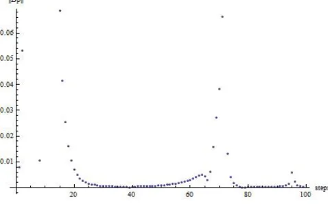
Thus using as starting point (t = 0) the degenerate com-pensatorKD we produced a set of 100 static compensators by applying the computational method as described in Algo-rithm 1 with∆t= 0.01. The errorsk∆pkbetween the actual closed-loop polynomial and the ideal one(s+1)11are shown in Figure 1. Note that, the compensators corresponding to small t have large norm and are the ones close to the degenerate point as demonstrated by the angle measure in Figure (2).
The compensator with the lower norm and hence with the lower sensitivity and with the maximum distance from the degenerate point (90 degrees) is given by
Kf =
−3.24468 −14.5316 −2.04266 −0.156795 49.0151 217.497 28.3229 6.23728
−4.16871 −23.7617 −2.97827 0.0136797
(18) and the resulting closed-loop characteristic polynomial is
1.+ 11.s+ 55.s2+ 165.s3+ 330.s4+ 462.s5+
+462.s6+ 330.s7+ 165.s8+ 55.s9+ 11.s10+ 1.s11
[image:7.612.316.558.52.207.2]The angle KD∠Kf (in degrees), between the degenerate
Fig. 1. Distance from the target closed loop polynomialp(s)vs.t
compensator KD and the final output feedback matrix Kf, as defined in (16) is θ= 90◦ and guarantees the maximum distance from the degenerate point and hence the lower sensitivity solution. The variation of angle θ for all the produced compensators is indicated in Figure (2).
B. Example 2
[image:7.612.366.504.268.316.2]Consider the system of p = 2 inputs, m = 2 outputs and n= 8states whose composite MFD of its transfer function
Fig. 2. Angle (in degrees) between degenerate compensator and the resulting output feedback matrix
is given by
M(s) =
D(s) N(s)
=
s4 0 s3 s4
s 1
1 0
Since mp = 4 < 8 = n the system does not have the arbitrary pole assignability property via SOF. The least degree family of controllers that satisfies condition (1) is nc = 2, such that 4 + 4nc > 8 +nc. Therefore, using a controller with 2 inputs, 2 outputs and 2 states it is desired to assign a closed-loop polynomial ofn+nc = 8 + 2 = 10 -th degree, given here for simplicity as(s+ 1)10 with a real coefficient vector∈R11.
p= [1,10,45,120,210,252,210,120,45,10,1]T
The dynamic problem given here will be transformed into an equivalent static one (of a higher dimension) by shifting the dynamics from K(s) toM(s) as shown in (5) and will be indicated next. Let K(s) = sK1 +K0 be the composite MFD of the controller, where K1, K0 are p×(m +p) constant coefficient matrices and q = 1 in order to satisfy the McMillan degree of the controller (i.e.nc =q·p= 2). Then, based on (5) we have that
[sK1+K0]
D(s) N(s)
= K1|K0
sD(s) sN(s) D(s) N(s)
are equivalent and the resulting static problem has a com-posite system matrix of a higher-degree with dimensions (q+ 1)(m+p)×p, i.e.2(2 + 2)×2 = 8×2, given as
˜ M(s) =
s5 s4 s2 s s4 s3 s 1 0 s5 s 0 0 s4 1 0
T
By considering the degenerate controller[KD1|KD0]∈R 2×8
KD(s) = [sKD1+KD0] =
1 −s 0 0 0 0 1 −s
=s
0 −1 0 0 0 0 0 −1
+
1 0 0 0 0 0 1 0
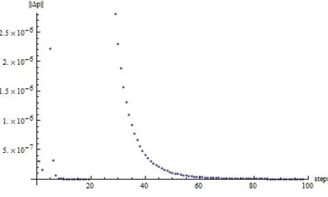
[image:7.612.56.295.441.590.2]as a starting point, we run the numerical method (as de-scribed in Algorithm 1), and a set of 100 controllers pro-duced. The errors, k∆pk, between the actual closed-loop polynomial and the ideal one (s+ 1)10 are summarised in Figure (3). In overall, were less than2×10−6 for allt.
Fig. 3. Distance from the target closed loop polynomialp(s)vs.t
The controller, Kf(s), with the maximum angle from KD(s), has the following composite MFD
0.546−0.279s 0.095−0.144s 0.078 + 0.132s 0.244 + 0.391s
0.275−0.129s 0.053−0.067s 0.118 + 0.111s 0.368 + 0.308s
whose transfer function matrix Kf(s) = Dc−1(s)Nc(s) is given by
0.00717s2 +0.0082s−0.00717 5.98×10⁻⁵s2 +5.98×10⁻⁴s+0.027
0.018s2 +0.028s−0.0223 5.98×10⁻⁵s2 +5.98×10⁻⁴s+0.027
−0.014s2 +0.0014s−0.043 5.98×10⁻⁵s2 +5.98×10⁻⁴s+0.027
−0.035s2−0.010s+0.134 5.98×10⁻⁵s2 +5.98×10⁻⁴s+0.027
which assigns the closed loop characteristic polynomial to
0.999999 + 10.s+ 45.s2+ 120.s3+ 210.s4+ 252.s5+
+210.s6+ 120.s7+ 45.s8+ 10.s9+ 1.s10
and has the following characteristics:
• Gap from degenerate compensator= 90◦ • M axSV[K1, K0] = 0.9985
• M inSV[K1, K0] = 0.0542
As before in Example 1, the angle KD∠Kf between the degenerate compensator and the final output feedback matrix isθ= 90◦. The angle for all the produced controllers versus t are shown in Figure (4).
V. CONCLUSIONS
[image:8.612.57.295.135.278.2]An improvement of the Global Linearisation framework has been introduced, for the output feedback pole assignment problem, that allows to produce systematic solutions which improve the sensitivity characteristics of the methodology and its inherent dependence on degenerate compensators. The proposed numerical scheme for finding output feedback controllers is based on a quasi-Newton method modified accordingly to use the freedom that exists in order to achieve optimization goals while achieving pole placement. Here, the numerical method was adjusted to maximize the angle from the degenerate point and hence the distance from
Fig. 4. Angle (in degrees) between degenerate compensator and the resulting output feedback matrix
that in order to examine the sensitivity properties of such solutions. The results indicated that the solutions far from the degenerate point are indeed the ones with the lower sensitivity. Furthermore, the selection of the degenerate point around which global linearisation is achieved is a possible factor that affects the overall performance and hence the optimal selection of degenerate points needs to be further examined.
REFERENCES
[1] N. Karcanias and C. Giannakopoulos, “Grassmann invariants, almost zeros and the determinantal pole-zero assignment problems of linear systems,”International Journal of Control, pp. 673–698, 1984. [2] X. Wang, “Grassmannian, central projection and output feedback
pole assignment of linear systems,”IEEE Transactions on Automatic Control, vol. 41, no. 6, pp. 786–794, 1994.
[3] J. Rosenthal, J. Schumacher, and J. Willems, “Generic eigenvalue assignment by memoryless real output feedback,”Systems and Control Letters, vol. 26, pp. 253–260, 1995.
[4] S. Ariki, “Generic pole assignment via dynamic feedback,” SIAM Journal on Control and Optimization, vol. 36, no. 1, 1998. [5] J. Rosenthal and X. Wang, “Output feedback pole placement with
dynamic compensators,” IEEE Transactions on Automatic Control, vol. 41, pp. 775–795, 1996.
[6] X. Wang, “Pole placement by static output feedback,”J.Math. Sys. Estim. Control, vol. 2, p. 205, 1992.
[7] J. Leventides and N. Karcanias, “Dynamic pole assignment using global blow up linearisation: Low complexity solution,” Journal of Optimization Theory and Applications, 1998.
[8] J. Leventides, “Algebrogeometric and topological methods in control theory,” PhD Thesis, Control Engineering Centre, City University, 1993.
[9] J. Leventides and N. Karcanias, “Global asymptotic linearisation of the pole placement map: a closed form solution of the output feedback problem,”Automatica, pp. 1303–1309, 1995.
[10] R. Brockett and C. Byrnes, “Multivariable nyquist criterion, root loci and pole placement:a geometric viewpoint,”IEEE Trans. Aut. Control, vol. AC–26, pp. 271–283, 1981.
[11] N. Karcanias, J. Leventides, and I. Meintanis, “Parameterisation of degenerate solutions of the determinantal assignment problem,” in
Proc. IFAC Symposium on Systems Structure and Control (SSSC2013), France, 4–6 Feb. 2013.