Almost sure stability of the Euler–Maruyama
method with random variable stepsize for stochastic
differential equations
Wei Liu1∗ Xuerong Mao2
1 Department of Mathematics,
Shanghai Normal University, Shanghai, 200234, China.
2 Department of Mathematics and Statistics,
University of Strathclyde, Glasgow G1 1XH, U.K.
Abstract
In this paper, the Euler–Maruyama (EM) method with random variable stepsize is studied to reproduce the almost sure stability of the true solutions of stochastic differential equations. Since the choice of the time step is based on the current state of the solution, the time variable is proved to be a stopping time. Then the semimartingale convergence theory is employed to obtain the almost sure stability of the random variable stepsize EM solution. To our best knowledge, this is the first paper to apply the random variable stepsize (with clear proof of the stopping time) to the analysis of the almost sure stability of the EM method.
Key words: stopping time, almost sure stability, Euler–Maruyama, variable stepsize, semi-martingale convergence theory.
1
Introduction
This paper is devoted to the analysis of the numerical reproduction of the almost sure stability for stochastic differential equations (SDEs) by using the well-known semimartingale convergence theory. Almost sure stability of solutions to SDEs has been widely studied (see for example, Chapter 5.8 in [9], Chapter 4.3 in [12], and the references therein). The ability to reproduce the almost sure stability is one important characteristic of numerical methods. Many papers have
∗
studied the numerical reproduction of the almost sure stability by adopting the semimartingale convergence theory, for example [2, 14, 19, 20, 23, 24, 25] and the references therein. However, in most of the papers the stepsize is either fixed or nonrandom variable.
The classical explicit methods, such as the Euler-Maruyama method, may reproduce the almost sure stability of SDEs with the global Lipschitz coefficients, but the requirements on the time stepsize are very restrictive. For SDEs with non-global Lipschitz coefficient, the Euler-Maruyama method may not preserve this properties with any stepsize (see for example Lemma 3.1 in [8]). To tackle this, the methods with implicit structure are often employed as the alternatives [13, 19, 23]. Compared with the classical explicit methods, those implicit methods can reproduce larger ranges of SDEs with less restrictions on the stepsize. Nevertheless, the implicit methods may require additional computational costs to solve nonlinear equation system at each iteration.
Bearing those points above in mind, the random variable stepsize is introduced to embed into the classic Euler-Maruyama (EM) method in this paper. Our key contribution is that we prove the time variable is a stopping time. Moreover, the stopping time is essential for the application of the semimartingale convergence theory in our approach. Benefiting from the random variable stepsize, the sufficient conditions for the almost sure stability of the EM method obtained in this paper are much weaker than those established in [14] and [23]. To our best knowledge, this is the first paper to apply the random variable stepsize (with clear proof of the stopping time) to the analysis of the almost sure stability of the EM method.
It should be noted that the technique of adjusting the size of each step has been broadly used in the multi-stage methods (see for example [3, 4, 18], and references therein). Due to the application of the local error control technique, some steps could be rejected then smaller steps may be retreated. Since the stepsize in those methods is dependent on the state of the solution, it is indeed a random variable. However, the current stepsize may be decided after future information available and this indicates the time variable can not be a stopping time [15]. In fact, not like the case in this paper the stopping time is not necessary for those methods [6].
The Euler-type methods with the random variable stepsize, were also considered in different aspects, for instance in [5] to reproduce the finite time explosion of SDEs, in [11] to study convergence and ergodicity, and in [16] to optimise the error constant.
applying the the strong law of large numbers, and by the Chebyshev inequality and the Borel-Cantelli lemma the almost sure stability can be derived from the moment exponential stability. We refer to some of the works [8, 10, 13, 17, 21] and references therein.
This paper is constructed as follows. Section 2 is devoted to the mathematical notation and some preparation for the main result. In Section 3 we present our main result, Theorem 3.1, in which we demonstrate the strategy of choosing the stepsize, give the proof of the stopping time and conclude the almost sure stability of the EM method with random variable stepsize. Section 4 sees the computer simulations of the proposed method. In Section 5, alternative sufficient conditions for the numerical almost sure stability are proposed, which enable the EM method with random variable stepsize to cover wider range of SDEs. Proofs in the last section are only briefed as the same techniques to those in Theorem 3.1 are employed.
2
Preliminary
Throughout this paper, let (Ω,F,{Ft}t≥0,P) be a complete probability space with a filtration
{Ft}t≥0 which is increasing and right continuous, withF0 containing allP-null sets. LetB(t) =
(B1(t), ..., Bm(t))T be an m-dimensional Brownian motion defined on the probability space, whereT denotes the transpose of a vector or a matrix. Let| · |denote both the Euclidean vector norm and the Frobenius matrix norm. The inner product of x, y in Rn is denoted by hx, yi.
Denote max(a, b) and min(a, b) by a∨b and a∧b, respectively. Denote the smallest integer larger than a real number x by dxe. R+ denotes the set of all nonnegative real numbers. N
denotes the set of all nonnegative integers. Z denotes the set of all integers. Qdenotes the set
of all rational numbers.
In this paper, we investigate the numerical methods for the n-dimensional SDE
dx(t) =f(x(t))dt+g(x(t))dB(t), x(0)∈Rn, (2.1) wheref: Rn→Rn and g: Rn→Rn×m. The following two conditions are imposed on the drift
and diffusion coefficients. For every integer R ≥1, there exists a positive constant C(R) such that, for all x, y∈Rn with|x| ∨ |y| ≤R,
|f(x)−f(y)|2∨ |g(x)−g(y)|2≤C(R)|x−y|2. (2.2) And ∀x∈Rn
From (2.3), we can see that the coercivity condition holds automatically. Therefore under (2.2) and (2.3), there exists a unique solution to (2.1) for any given initial valuex(0)∈Rn(see, for example Theorem 2.3.5 in [12]). The theorem for the almost sure asymptotic stability for the SDE (2.1) is presented as follows.
Theorem 2.1 Let (2.2) and (2.3) hold. Assume z(x) = 0 if and only if x = 0, then for any initial value x(0)∈Rn
lim
t→∞x(t) = 0 a.s.
We refer to the stochastic version of the LaSalle theorem in [22] for the proof of this theorem.
Lemma 2.2 Assume z(x), defined by (2.3), is zero if and only if x = 0. Then both f(x) = 0 and g(x) = 0 if x= 0, and f(x)6= 0 if x6= 0.
Proof. We first prove f(x) 6= 0 if x 6= 0. Assume f(¯x) = 0 for some ¯x 6= 0, then by (2.3) we have −z(¯x) =|g(¯x)|2 ≥0. But this contradicts that−z(x)<0 for x6= 0.
We now prove f(x) = 0 if x = 0. Assumef(0)6= 0, that is f(0) = (f1(0), ..., fn(0))T 6= 0. Without loss of generality, we assume f1(0) < 0. Due to the continuity of f(x), for some sufficiently smallε >0 we havef1(x)<0 for some vectorx, where the first entry lies in (−ε, ε) and all the rest are zeros. Then given ¯x = (−ε/2,0, ...,0)T, we have hx, f¯ (¯x)i > 0. But this contradicts to−z(¯x)<0.
Suppose x= 0, by (2.3) it is easy to see that|g(0)|2 =−z(0) = 0, i.e. g(0) = 0.
The next lemma is a discrete version of the semimartingale convergence theorem. We refer the readers to Lemma 4 in [1] for the proof.
Lemma 2.3 Let {Ai} and {Bi} be two nonnegative Fi-measurable processes for i= 0,1,2, ... withA0 =B0= 0a.s. and{Mi}beFi-measurable local martingale fori= 0,1,2, ...withM0 = 0. If a nonnegative stochastic process {Zi}i=0,1,... can be decomposed as Zi =Z0+Ai−Bi+Mi, then
lim
i→∞Ai <∞
⊆
lim
i→∞Bi<∞
∩
lim
i→∞Zi exists and is finite
a.s.
3
The EM method with random variable stepsize
notice that there are other choices. We emphasise here that there are two important properties of the variable stepsize that the sum of the steps is a stopping time and divergent. The feature of stopping time is essential to the proof of the local martingale term in Theorem 3.1, and the divergence guarantees the time is able to tend to infinity.
The first main result is that the variable stepsize method can reproduce the stability of the SDE shown in Theorem 2.1.
Theorem 3.1 Let (2.2) and (2.3) hold. Assume z(x) = 0 if and only if x= 0, and lim inf
|x|→0
z(x)
|f(x)|2 >0. (3.1) Define the EM method with variable stepsize as
Yi+1=Yi+f(Yi)∆ti+g(Yi)∆Bi, Y0 =x(0), i≥0, (3.2) where ∆Bi =B(ti)−B(ti−1) with ti = Pik=0∆tk for i = 0,1,2... and t−1 = 0, ∆ti is chosen to be 2−ni with n
i =d1−log2(z(Yi)/|f(Yi)|2)e for |Yi| 6= 0 and 2−2 for |Yi|= 0. Then ti is an {Ft}-stopping time for each i = 0,1,2..., and the sequence of time steps obeys P∞i=0∆ti = ∞ a.s. Moreover, for any initial valueY0 ∈Rn
lim
i→∞Yi = 0 a.s. Proof. Taking square on both sides of (3.2), we have
|Yi+1|2 = |Yi|2+ 2hYi, f(Yi)∆ti+g(Yi)∆Bii+|f(Yi)∆ti+g(Yi)∆Bi|2
= |Yi|2+ ∆ti(2hYi, f(Yi)i+|g(Yi)|2+|f(Yi)|2∆ti) + ∆mi, (3.3) where ∆mi = 2hYi, g(Yi)∆Bii+ 2hf(Yi)∆ti, g(Yi)∆Bii+|g(Yi)|2(|∆Bi|2−∆ti).
The proof is divided into three parts. Firstly, we demonstrate the strategy of choosing the stepsize ∆ti in each time step and show that ti is an {Ft}-stopping time for every i= 0,1, .... Then we prove that mi =Pik=0∆mk is a local martingale fori= 0,1, .... At last, we give the proof of the divergence of the sequence of the timesteps and conclude the almost sure stability.
Step 1
For example, when Yi 6= 0 (by Lemma 2.2 we know f(Yi) 6= 0) we could choose ∆ti = 2−ni with ni =d1−log2(z(Yi)/|f(Yi)|2)e. Then it is obvious that ∆ti ≤z(Yi)/(2|f(Yi)|2), thus the inequality (3.4) holds. WhenYi = 0 (i.e. z(Yi) = 0 andf(Yi) = 0), any choice of ∆ti will satisfy (3.4) and we simply choose, for example ∆ti = 2−2. From the iteration (3.2), we know that if at some time point the solution becomes zero, the solution afterwards will stay at zero. Hence in this case the stepsize is fixed and the almost sure stability follows naturally. In the following, we focus on the case when ∆ti = 2−ni with ni = d1−log2(z(Yi)/|f(Yi)|2)e. We emphasise here that the requirement that each ∆ti is a rational number is key to the following proof that
ti =Pik=0∆tk=Pik=02−nk is an {Ft}-stopping time for every i= 0,1, ....
Assume ti is an {Ft}-stopping time for some i≥0, i.e. {ti ≤t} ∈ Ft for any t≥0. Note that Yi+1 is Fti-measurable. Because the choice of ∆ti+1 is dependent on Yi+1 we have that
∆ti+1 is Fti-measurable. Then we need to show ti+1 = ti+ ∆ti+1 is an {Ft}-stopping time,
that is to show {ti + ∆ti+1 ≤ t} ∈ Ft for any t ≥ 0. For any s ∈ Z and any j ∈ N with
j2s ∈[0, t], we have {ti ≤j2s} ∈ Fj2s ⊆ Ft, and {∆ti+1 ≤t−j2s} ∈ Ft
i ⊂ F. Thus we have
{ti ≤j2s} ∩ {∆ti+1≤t−j2s} ∈ Ft(see for example [12]). As bothZand Nare countable sets,
we have that for anyt≥0 [7] {ti+ ∆ti+1≤t}=
[
{0≤j2s≤t,s∈ Z,j∈N}
({ti≤j2s} ∩ {∆ti+1 ≤t−j2s})∈ Ft.
Thus we have proved thatti+1 is an {Ft}-stopping time. Since ∆t0 is dependent on the given initial value Y0, we have ∆t0 and Y0 areFt−1-measurable (recalling t−1 = 0). By induction we
conclude thatti is an {Ft}-stopping time for each i= 0,1, .... Substituting (3.4) into (3.3), we obtain
|Yi+1|2 =|Yi|2−U(Yi,∆ti)∆ti+ ∆mi. Then taking sum on iwe have
|Yi+1|2=|Y0|2− i X
k=0
U(Yk,∆tk)∆tk+mi, (3.5)
wheremi=Pik=0∆mk. Step 2
Due to (3.2) and the definition ofti, it is clear thatYi isFti−1-measurable fori= 0,1, .... We
de-fine another filtration{Gi}i=−1,0,1,... byGi =Fti fori=−1,0,1, .... SoYi isGi−1-measurable and
R s.t. |x(0)|< R, we define a stopping time
ρR= inf{i≥0,|Yi|> R}.
Clearly, ρR → ∞ a.s. when R → ∞. It is easy to see that ρR is a {Gi−1}-stopping time i.e. {ρR ≤ i} ∈ Gi−1. This indicates {ρR−1 ≤ i} ∈ Gi. Denoting τR = ρR−1, we have τR is a {Gi}-stopping time. By the definition of ρR, we have that |Yi∧(ρR−1)| ≤R a.s. and |Yi∧τR| ≤R
a.s. for all i≥0.
We claim thatti∧τR andt(i−1)∧τR are{Ft}-stopping times. Forti∧τR we have for anyt≥0
{ti∧τR ≤t}={{ti ≤t} ∩ {τR≥i}} ∪ {{tτR ≤t} ∩ {τR< i}}.
Since {τR≥i} ∈ Gi−1 ⊂ Gi=Fti, we have {ti ≤t} ∩ {τR≥i} ∈ Ft. And
{tτR ≤t} ∩ {τR< i}=
i−1 [
j=0
({{tj ≤t} ∩ {τR=j}),
because {τR = j} ∈ Fti for j = 0,1, ...i−1 we have {tτR ≤ t} ∩ {τR < i} ∈ Ft. Hence
{ti∧τR ≤t} ∈ Ft. Similarly for t(i−1)∧τR, we have
{t(i−1)∧τR ≤t}={{ti−1 ≤t} ∩ {τR≥i−1}} ∪ {{tτR ≤t} ∩ {τR< i−1}}.
Since {τR≥i−1} ∈ Gi−2 ⊂ Fti, we have {ti−1 ≤t} ∩ {τR≥i−1} ∈ Ft. And
{tτR ≤t} ∩ {τR< i−1}=
i−2 [
j=0
({{tj ≤t} ∩ {τR=j}),
we have{{tτR ≤t} ∩ {τR< i−1}} ∈ Ft due to {τR=j} ∈ Gj ⊂ Fti forj = 0,1, ...i−2. Thus
{t(i−1)∧τR ≤t} ∈ Ft.
Due to the iteration (3.2) and the fact that |Yk∧τR|= |YτR| for any k ≥τR, we define the
Brownian motion increment with the stopping time by ∆Bi∧τR = B(ti∧τR)−B(t(i−1)∧τR) and
the time step with the stopping time by ∆ti∧τR = ti∧τR −t(i−1)∧τR. Since τR → ∞ a.s. when
R → ∞, those two definitions can reproduce the original ones we used in the statement of the theorem. Thus they are valid. In addition, we have
mi∧τR =
i∧τR
X
k=0
∆mk= i X
k=0
∆mk∧τR and mi∧τR =m(i−1)∧τR+ ∆mi∧τR.
on R such that|f(x)| ∨ |g(x)| ≤c(R). By the elementary inequality, we have |mi∧τR| =
i∧τR X k=0 ∆mk
≤ i X k=0
|∆mk∧τR|
≤ i X
k=0
(2|Yk∧τR||g(Yk∧τR)||∆Bk∧τR|+ 2|f(Yk∧τR)||g(Yk∧τR)|∆tk∧τR|∆Bk∧τR|
+|g(Yk∧τR)|
2||∆B k∧τR|
2−∆t k∧τR|)
≤ i X
k=0
(c1(R)|∆Bk∧τR|+c2(R)|∆Bk∧τR|
2), (3.6)
wherec1(R) and c2(R) are constants dependent on R only. Hence we have
E|mi∧τR| ≤
i X
k=0
(c1(R)E|∆Bk∧τR|+c2(R)E|∆Bk∧τR|
2)<∞. Also we have
E(mi∧τR
Gi−1) =E(m(i−1)∧τR+ ∆mi∧τR
Gi−1) =m(i−1)∧τR +E(∆mi∧τR
Gi−1). (3.7) Because {τR> i−1} ∈ Gi−1 and ∆Bi is independent of Gi−1, we have
E(∆Bi∧τR
Gi−1)
= E[(B(ti)−B(ti−1))1{τR>i−1}
Gi−1] +E[(B(tτR)−B(tτR))1{τR≤i−1}
Gi−1] = 1{τR>i−1}E[B(ti)−B(ti−1)]
= 0,
E(|∆Bi∧τR|
2 Gi−1)
= E[|B(ti)−B(ti−1)|21{τR>i−1}
Gi−1] +E[|B(tτR)−B(tτR)|21{τ
R≤i−1}
Gi−1]
= 1{τR>i−1}E[|B(ti)−B(ti−1)|2] = 1{τR>i−1}(ti−ti−1),
and
E(∆ti∧τR
Gi−1) = ∆ti∧τR
= 1{τR>i−1}(ti−ti−1) +1{τR≤i−1}(tτR −tτR)
Hence
E(∆mi∧τR
Gi−1)
= E(2hYi∧τR, g(Yi∧τR)∆Bi∧τRi+ 2hf(Yi∧τR)∆ti∧τR, g(Yi∧τR)∆Bi∧τRi
+|g(Yi∧τR)|
2(|∆B i∧τR|
2−∆t i∧τR)
Gi−1) = 2hYi∧τR, g(Yi∧τR)iE(∆Bi∧τR
Gi−1) + 2hf(Yi∧τR), g(Yi∧τR)i∆ti∧τRE(∆Bi∧τR
Gi−1) +|g(Yi∧τR)|
2(
E(|∆Bi∧τR|
2
Gi−1)−E(∆ti∧τR
Gi−1))
= 0. (3.8)
Combining (3.7) and (3.8), we achieve the required
E(mi∧τR
Gi−1) =m(i−1)∧τR.
This means that {mi∧τR}i≥0 is a {Gi}-martingale. Recalling that τR→ ∞ a.s. when R → ∞,
we see that{mi}i≥0 is a{Gi}-local martingale. Step 3
Therefore from (3.5) and Lemma 2.3, we have
lim i→∞|Yi|
2<∞ a.s. (3.9)
and
∞ X
k=0
U(Yk,∆ti)∆tk<∞ a.s. (3.10) From (3.10), we have limi→∞U(Yi,∆ti)∆ti = 0 a.s. We next show the time step ∆ti will never tend to zero as igoes to infinity, that is lim infi→∞∆ti>0 a.s.
According to (3.9) for almost all ω∈Ω, there existsC(ω)∈R+ such that limi→∞|Yi(ω)|=
C(ω). Fix any suchω, write C(ω) =C and Yi(ω) =Yi. Consider two cases:
(i) For the case when C 6= 0, there exists a sufficiently large integer i∗1 such that for all
i > i∗1, 0.5C < |Yi|< 1.5C. This indicates either 0.5C < Yi < 1.5C or −1.5C < Yi <−0.5C. Because that z(x) = 0 and f(x) = 0 if and only ifx = 0, in both of the two intervals we have
z(Yi)6= 0 and f(Yi)6= 0. Furthermore, due to the continuity ofz(x) and f(x), we have min
0.5C≤|x|≤1.5C
z(x)
|f(x)|2 =η >0. So for any i > i∗1, we have
z(Yi) |f(Yi)|2
then
1−log2(z(Yi)/|f(Yi)|2)≤1−log2(η). Recalling the choice of the stepsize, we see
ni =d1−log2(z(Yi)/|f(Yi)|2)e ≤ d1−log2(η)e then
∆ti = 2−ni ≥2−d1−log2(η)e>0.
(ii) For the case when C= 0, suppose the limit of (3.1) be D >0. There exists a constant
δ = δ(D) > 0 such that |z(x)/|f(x)|2 −D| < 0.5D for all |x| ∈ (0, δ). Also, there exists an integeri∗2 such that for alli > i∗2, |Yi| ∈(0, δ), which indicates|z(Yi)/|f(Yi)|2−D|<0.5D. So for any i > i∗2, we have
1−log2(1.5D)<1−log2(z(Yi)/|f(Yi)|2)<1−log2(0.5D). Recalling the choice of the stepsize, we see
∆ti= 2−ni >2−d1−log2(0.5D)e>0.
Thus ∆ti will never tend to 0 asitends to infinity. Hence we have P∞i=0∆ti=∞ a.s.
Now we have limi→∞U(Yi,∆ti) = 0 a.s. Due to (3.4) and the choice of ∆ti that ∆ti ≤
z(Yi)/(2|f(Yi)|2), we have
U(Yi,∆ti) =z(Yi)− |f(Yi)|2∆ti ≥0.5z(Yi)≥0.
Therefore limi→∞z(Yi) = 0 a.s. Given the condition “z(x) = 0 ⇔ x = 0”, we obtain that limi→∞Yi = 0 a.s. Hence the proof is complete.
We have three comments on the proof.
• The conditions in Theorem 3.1 for the EM method with variable stepsize is weaker than
the condition for the EM method with fixed stepsize (i.e. when θ= 0) stated in Theorem 5.3 of [14]. For example, a scalar SDEdx(t) = (−x3(t)−x(t))dt+x2(t)dB(t) satisfies the conditions in Theorem 3.1, but not in Theorem 5.3 of [14].
• When conducting computer simulation, the stepsize is naturally rational number as
• The condition (2.3) is the restriction on the relation between the drift and the diffusion coefficients, which is also required for the almost sure stability of the underlying SDEs. The condition (3.1) is solely required for the numerical methods. From the proof, we can see that (3.1) guarantees the sum of the sequence of stepsizes tends to infinity. This is essential as we are discussing asymptotic behaviour of the numerical solution.
Theorem 3.2 Let (2.2) and (2.3) hold. Assume z(x) = 0 if and only if x = 0, and (3.1). For the EM method with variable stepsize (3.2), ∆ti is chosen to be rational number satisfying ∆ti = αz(Yi)/(|f(Yi)|2) with α ∈ (0,1) for |Yi| 6= 0, and any nonzero rational number for |Yi|= 0. Thenti is an {Ft}-stopping time for each i= 0,1,2..., and the sequence of time steps obeys P∞
i=0∆ti =∞ a.s. Moreover, for any initial valueY0 ∈Rn
lim
i→∞Yi = 0 a.s.
Most part of the proof of Theorem 3.2 is similar to the proof of Theorem 3.1, and the only different part is the proof of the stopping time as follows.
Assume ti is an {Ft}-stopping time for some i≥0, i.e. {ti ≤t} ∈ Ft for any t≥0. Note that Yi+1 is Fti-measurable, because the choice of ∆ti+1 is dependent on Yi+1 we have that
∆ti+1 isFti-measurable. Then we need to showti+1 =ti+ ∆ti+1is an{Ft}-stopping time, that
is to show {ti+ ∆ti+1 ≤ t} ∈ Ft for any t ≥ 0. For any rational number s ∈ [0, t], we have {ti ≤s} ∈ Fs⊆ Ft, and{∆ti+1 ≤t−s} ∈ Fti ⊆ F. Thus we have{ti ≤s}∩{∆ti+1≤t−s} ∈ Ft
(see for example [12]). As the set of all rational number s ∈ [0, t] is a countable set, we have that for anyt≥0 [7]
{ti+ ∆ti+1 ≤t}=
[
{0≤s≤t,s∈Q}
({ti≤s} ∩ {∆ti+1≤t−s})∈ Ft.
Thus we have proved thatti+1 is an {Ft}-stopping time. Since ∆t0 is dependent on the given initial value Y0, we have ∆t0 and Y0 areFt−1-measurable (recalling t−1 = 0). By induction we
conclude that ti is an{Ft}-stopping time for eachi= 0,1, ....
4
Examples
We first consider a scalar SDE
with a given initial valuex(0) = 1. It is easy to verify that for anyx∈Rwithx6= 0
−z(x) := 2hx, f(x)i+g2(x) =−2x2−x4 <0.
It is clear that ”z(x) = 0⇔x= 0”, by Theorem 2.1 we have the solution of the underlying SDE is asymptotically almost surely stable. Moreover,
[image:12.612.123.472.406.538.2]lim inf |x|→0
z(x)
|f(x)|2 = lim inf|x|→0
2x2+x4
x2+ 2x4+x6 = 2>0.
Choose the stepsize, for example ∆ti = 0.98z(Yi)/|f(Yi)|2 in each step, from Theorem 3.2 we obtain the variable stepsize EM solution is asymptotically almost surely stable as well. Set
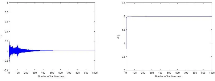
Y0 = 1, we simulated 1000 time steps of one path of the variable stepsize EM solution. The left plot on Figure 1 is the solution path, from which we can see that the oscillation decays and the solution tends zero as time increases. This is in line with the theoretical result. The plot on the right of Figure 1 is the size of each time step. It is clear that with the solution approaching the origin the stepsize tends to 1.96 and this is due to the limit 2 and the choice of factor 0.98. In addition, the plot also shows that the stepsize does not need to tend to zero, thus we have
P∞
i=0∆ti=∞ a.s.
Figure 1: Left: One simulation path, Right: The stepsize of each time step
Now we consider a two-dimensional case
dx(t) = diag(x1(t), x2(t)) ((b+Adiag(x1(t), x2(t))x(t))dt+σdB(t)), (4.2) where diag(x1(t), x2(t)) denotes diagonal matrix with nonzero entries x1(t) and x2(t) on the diagonal, x(t) = (x1(t), x2(t))T, b = (b1, b2)T, A = (aij)i,j∈{1,2}, σ = (σij)i,j∈{1,2} and B(t) = (B1(t), B2(t))T.
−1. It is easy to verify that for anyx∈R2 andx6= 0
2hx, f(x)i+g2(x)
= (2b1+σ211+σ212)x21+ (2b2+σ221+σ222)x22+ (a12+a21)x21x22+a11x41+a22x42<0. From Theorem 2.1, we know the SDE solution is almost surely stable. In addition, by the elementary inequality ab≤a2+b2 we have
[image:13.612.128.472.355.486.2]lim inf |x|→0
z(x) |f(x)|2 = lim inf
|x|→0
1.5x21+ 2x22+x21x22+x41+x42
x21+ 2x41+x61+ 2x21x42+ 5x41x22+ 4x22+ 4x42+x62
≥ lim inf |x|→0
|x|2
4|x|2+ 6.5|x|4+|x|6+ 2.5|x|8 = 1
4 >0.
By choosing the stepsize, for example ∆ti = 0.1z(Yi)/|f(Yi)|2 in each step, we have from Theo-rem 3.1 that the variable stepsize EM solution is almost surely stable as well.
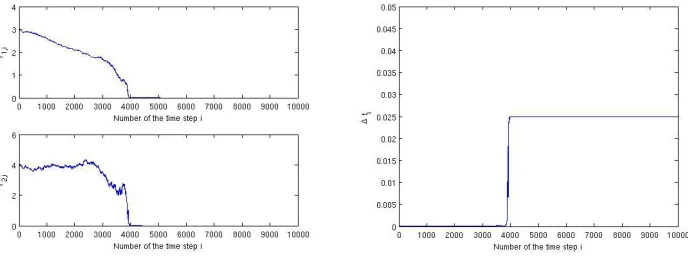
Figure 2: Left: One simulation path of Y1,· and Y2,·, Right: The stepsize of each time step.
We simulated 10000 time steps and plotted the two solution paths on the left of Figure 2. It can be seen that as time increases both the solutions tend to zero. And from the plot on the right of Figure 2 the size of the time step approaches to 0.025 as the solutions go to zeros, which shows the stepsize will not tend to zero. Hence both the simulations of the one-dimensional and the multi-dimensional cases are in line with the theoretical result.
5
Other sufficient conditions
Another condition that can be regarded as an extension to (2.3) is to assume there exists a symmetric positive-definiten×n matrixQsuch that for ∀x∈Rn
−z¯(x) := 2xTQf(x) +trace(gT(x)Qg(x))≤0. (5.1) It is clear to see that whenQis an identity matrix, (2.3) is recovered. Thanks to the stochastic version of the LaSalle theorem in [22], we have that the underlying solution of (2.1) is almost surely asymptotically stable if (2.2) and (5.1) hold, and ¯z(x) = 0 if and only if x = 0. In addition, it is obvious that given the condition that ¯z(x) = 0 if and only if x = 0 the results in Lemma 2.2 still hold for f(x) andg(x). Denote the smallest and largest eigenvalue ofQ by
λmin(Q) andλmax(Q) respectively. Now we are ready to present the following theorem. Theorem 5.1 Let (2.2) and (5.1) hold. Assume z¯(x) = 0 if and only if x= 0, and
lim inf |x|→0
¯
z(x) |f(x)|2 >0.
For the EM method with variable stepsize (3.2), ∆ti is chosen to be rational number satisfying ∆ti = αz¯(Yi)/(λmax(Q)|f(Yi)|2) with α ∈ (0,1) for |Yi| 6= 0, and any nonzero rational number for |Yi|= 0. Then ti is an {Ft}-stopping time for each i = 0,1,2..., and the sequence of time steps obeys P∞
i=0∆ti =∞ a.s. Moreover, for any initial valueY0∈Rn
lim
i→∞Yi = 0 a.s.
Proof. Since Qis a symmetric positive-definite n×n matrix, it is clear that for anyi≥0
λmin(Q)|Yi|2 ≤YiTQYi≤λmax(Q)|Yi|2 and
λmin(Q)|f(Yi)|2 ≤fT(Yi)Qf(Yi)≤λmax(Q)|f(Yi)|2. From (3.2) we have
Yi+1T QYi+1 =YiTQYi+ ∆ti[2YiTQf(Yi) +trace(gT(Yi)Qg(Yi)) +fT(Yi)Qf(Yi)∆ti] + ∆mi, where
We see condition (5.1) as a generalisation of (2.3) as we can recover (2.3) by choosing Qto be identity matrix in (5.1).
To keep the notations simple in the next theorem, we investigate the SDEs with the scalar Brownian motion
dx(t) =f(x(t))dt+g(x(t))dB(t), x(0)∈Rn,
where f: Rn → Rn, g: Rn → Rn and B(t) is a scalar Brownian motion. We still assume
condition (2.2), but replace condition (2.3) by the following condition: there exists a constant
p∈(0,2) such that
−v:= sup x∈Rn,x6=0
2hx, f(x)i+|g(x)|2
|x|2 + (p−2)
hx, g(x)i2 |x|4
<0. (5.2) Also we assume f(0) = 0 and g(0) = 0.
Under (2.2) and (5.2), the true solution of SDE (2.1) is almost surely asymptotically stable [22]. Now we study the numerical solution.
Theorem 5.2 Let (2.2) and (5.2) hold. Assume
lim sup |x|→0
|f(x)|
|x| <∞, (5.3)
and
lim sup |x|→0
|g(x)|
|x| <∞. (5.4)
Define the EM method with variable stepsize as
Yi+1=Yi+f(Yi)∆ti+g(Yi)∆Bi, Y0 =x(0), i≥0, (5.5) where ∆Bi =B(ti)−B(ti−1) with ti=Pk=0i ∆tk for i= 0,1,2... andt−1 = 0. For Yi6= 0, ∆ti is chosen to be rational number satisfying ∆ti ≤(p/12) min{j=1,2,3,4,5}{(v/Aj(Yi))(1/j)}, where {Aj}j=1,2,3,4,5 are defined in the proof. For Yi = 0, ∆ti is chosen to be any nonzero rational number. Then ti is an {Ft}-stopping time for each i= 0,1,2..., and the sequence of time steps obeys P∞
i=0∆ti =∞ a.s. Moreover, for any initial valueY0 ∈Rn lim
i→∞Yi = 0 a.s.
The proof of this theorem is tedious but nontrivial. Therefore, we put it in Appendix.
covered by Theorem 3.1. But it should be noted that Theorem 3.1 is not fully included in Theorem 5.2. For example a scalar SDE withf(x) =−0.5x3−x5 andg(x) =x2. We check the conditions (2.3) and (3.1) that for any x∈Rn withx6= 0
2hx, f(x)i+g2(x) =−2x6 <0 and lim inf |x|→0
z(x) |f(x)|2 =
2 0.25 >0,
i.e. all the conditions in Theorem 3.1 hold. To check the condition (5.2) in Theorem 5.2, we have
2hx, f(x)i+|g(x)|2
|x|2 + (p−2)
hx, g(x)i2 |x|4 =−x
4+ (p−2)x2. But for anyp∈(0,2), we can not find av >0 to satisfy (5.2).
6
Conclusions
In this paper, we investigate the Euler–Maruyama method with random variable stepsize and successfully reproduce the almost sure stability of the true solution using this method with the semimartingale convergence theorem. Conditions we impose on the drift and diffusion coeffi-cients for the random variable stepsize method are much weaker than those for the fixed or nonrandom variable stepsize methods. Our key contribution also goes to the proof that the time variable is a stopping time, and only when this is true the rest of our proof is proper.
Considering that the random variable stepsize method works well for the stability, it is interesting to investigate other asymptotic properties of this method. Other numerical methods with random variable stepsize, such as the stochasticθ-method, are also worth to investigate.
The order-of-convergence is also essential for numerical methods. We have been working on the order of convergence of this newly developed Euler-Maruyama method with random variable stepsize, but due to the page limit here we will report the results in a follow-up paper.
Appendix
Proof of Theorem 5.2
From the first line of (3.3), we have that for the p given in (5.2) andYi 6= 0 |Yi+1|p=|Yi|p 1 +
2hYi, f(Yi)∆ti+g(Yi)∆Bii+|f(Yi)∆ti+g(Yi)∆Bi|2 |Yi|2
!p/2
.
In the following we focus on the case that Yi 6= 0 for all i≥0. Let
ζ = 2hYi, f(Yi)∆ti+g(Yi)∆Bii+|f(Yi)∆ti+g(Yi)∆Bi| 2
|Yi|2
,
and by the fundamental inequality that for any ζ ≥ −1 (1 +ζ)p/2 ≤1 +p
2ζ+
p(p−2)
8 ζ
2+p(p−2)(p−4) 23×3! ζ
3, we have
|Yi+1|p ≤ |Yi|p
1 +p 2ζ+
p(p−2)
8 ζ
2+p(p−2)(p−4) 23×3! ζ
3
. (6.1)
We compute
ζ = 1 |Yi|2
(∆ti(2hYi, f(Yi)i+|g(Yi)|2) + ∆t2i|f(Yi)|2
+2hYi, g(Yi)i∆Bi+ 2fT(Yi)g(Yi)∆ti∆Bi+|g(Yi)|2(∆Bi2−∆ti)),
ζ2 = 1 |Yi|4
(∆ti(4hYi, g(Yi)i2)
+∆t2i(4hYi, f(Yi)i2+|g(Yi)|4+ 4hYi, f(Yi)i|g(Yi)|2+ 8hYi, g(Yi)ifT(Yi)g(Yi)) +∆t3i(6|f(Yi)|2|g(Yi)|2+ 4hYi, f(Yi)i|f(Yi)|2) + ∆t4i|f(Yi)|4
+4hYi, g(Yi)i2(∆B2i −∆ti) +|g(Yi)|4(∆Bi4−∆t2i) + 4hYi, f(Yi)i|g(Yi)|2∆ti(∆Bi2−∆ti) +8hYi, g(Yi)ifT(Yi)g(Yi)∆ti(∆Bi2−∆ti) + 6|f(Yi)|2|g(Yi)|2∆t2i(∆Bi2−∆ti)
and
ζ3 = 1 |Yi|6
(∆t2i(24hYi, f(Yi)ihYi, g(Yi)i2+ 12hYi, g(Yi)i2|g(Yi)|2)
+∆t3i(8hYi, f(Yi)i3+ 12hYi, f(Yi)i2|g(Yi)|2+ 48hYi, f(Yi)ihYi, g(Yi)ifT(Yi)g(Yi) +12hYi, g(Yi)i2|f(Yi)|2+ 6hYi, f(Yi)i|g(Yi)|4+|g(Yi)|6+ 24hYi, g(Yi)i|f(Yi)||g(Yi)|3) +∆t4i(12hYi, f(Yi)i2|f(Yi)|2+ 36hYi, f(Yi)i|f(Yi)|2|g(Yi)|2+ 15|f(Yi)|2|g(Yi)|4 +24hYi, g(Yi)i|f(Yi)|3|g(Yi)|)
+∆t5i(6hYi, f(Yi)i|f(Yi)|4+ 15|f(Yi)|4|g(Yi)|2) +∆t6i(|f(Yi)|6)
+24hYi, f(Yi)i2hYi, g(Yi)i∆t2i∆Bi+ 24hYi, f(Yi)ihYi, g(Yi)i2∆ti(∆Bi2−∆ti) +8hYi, g(Yi)i3∆Bi3+ 24hYi, f(Yi)i2fT(Yi)g(Yi)∆t3i∆Bi
+12hYi, f(Yi)i2|g(Yi)|2∆t2i(∆B2i −∆ti) +24hYi, f(Yi)ihYi, g(Yi)i|f(Yi)|2∆t3i∆Bi
+48hYi, f(Yi)ihYi, g(Yi)ifT(Yi)g(Yi)∆ti2(∆Bi2−∆ti)
+24hYi, f(Yi)ihYi, g(Yi)i|g(Yi)|2∆ti∆Bi3+ 12hYi, g(Yi)i2|f(Yi)|2∆t2i(∆Bi2−∆ti) +24hYi, g(Yi)i2fT(Yi)g(Yi)∆ti∆B3i + 12hYi, g(Yi)i2|g(Yi)|2(∆Bi4−∆t2i)
+24hYi, f(Yi)i|f(Yi)|2fT(Yi)g(Yi)∆t4i∆Bi+ 36hYi, f(Yi)i|f(Yi)|2|g(Yi)|2∆t3i(∆Bi2−∆ti) +24hYi, f(Yi)ifT(Yi)g(Yi)|g(Yi)|2∆t2i∆Bi3+ 6hYi, f(Yi)i|g(Yi)|4∆ti(∆Bi4−∆t2i)
+6|f(Yi)|4fT(Yi)g(Yi)∆t5i∆Bi+ 15|f(Yi)|4|g(Yi)|2∆t4i(∆Bi2−∆ti) +20|f(Yi)|2fT(Yi)g(Yi)|g(Yi)|2∆t3i∆Bi3
+15|f(Yi)|2|g(Yi)|4∆t2i(∆Bi4−∆ti2) + 6fT(Yi)g(Yi)|g(Yi)|4∆ti∆Bi5+|g(Yi)|6(∆B6i −∆t3i) +6hYi, g(Yi)i|f(Yi)|4∆t4i∆Bi+ 24hYi, g(Yi)i|f(Yi)|3|g(Yi)|∆t3i(∆Bi2−∆ti)
+36hYi, g(Yi)i|f(Yi)|2|g(Yi)|2∆t2i∆Bi3+ 24hYi, g(Yi)i|f(Yi)||g(Yi)|3∆ti(∆B4i −∆t2i) +6hYi, g(Yi)i|g(Yi)|4∆Bi5).
Then we can rearrange (6.1) into
where
−U1(∆ti, Yi) :=
p
2
2hYi, f(Yi)i+|g(Yi)|2 |Yi|2
+ p−2 4
4hYi, g(Yi)i2 |Yi|4
+ ∆ti
p
2
|f(Yi)|2 |Yi|2 +p(p−2)
8
4hYi, f(Yi)i2+|g(Yi)|4+ 4hYi, f(Yi)i|g(Yi)|2+ 8hYi, g(Yi)ifT(Yi)g(Yi) |Yi|4
+p(p−2)(p−4) 23×3!
24hYi, f(Yi)ihYi, g(Yi)i2+ 12hYi, g(Yi)i2|g(Yi)|2 |Yi|6
+ ∆t2i
p(p−2) 8
6|f(Yi)|2|g(Yi)|2+ 4hYi, f(Yi)i|f(Yi)|2 |Yi|4
+p(p−2)(p−4) 23×3! ×
8hYi, f(Yi)i3+ 12hYi, f(Yi)i2|g(Yi)|2+ 48hYi, f(Yi)ihYi, g(Yi)ifT(Yi)g(Yi) |Yi|6
+12hYi, g(Yi)i 2|f(Y
i)|2+ 6hYi, f(Yi)i|g(Yi)|4+|g(Yi)|6+ 24hYi, g(Yi)i|f(Yi)||g(Yi)|3 |Yi|6
+ ∆t3i
p(p−2) 8
|f(Yi)|4 |Yi|4
+p(p−2)(p−4) 23×3! ×
12hYi, f(Yi)i2|f(Yi)|2+ 36hYi, f(Yi)i|f(Yi)|2|g(Yi)|2 |Yi|6
+15|f(Yi)| 2|g(Y
i)|4+ 24hYi, g(Yi)i|f(Yi)|3|g(Yi)| |Yi|6
+ ∆t4i
p(p−2)(p−4) 23×3!
6hYi, f(Yi)i|f(Yi)|4+ 15|f(Yi)|4|g(Yi)|2 |Yi|6
+ ∆t5i
p(p−2)(p−4) 23×3!
|f(Yi)|6 |Yi|6
and
∆mi = |Yi|p(
1 |Yi|2
(2hYi, g(Yi)i∆Bi+ 2fT(Yi)g(Yi)∆ti∆Bi+|g(Yi)|2(∆Bi2−∆ti)) + 1
|Yi|4
(4hYi, g(Yi)i2(∆Bi2−∆ti)
+|g(Yi)|4(∆Bi4−∆t2i) + 4hYi, f(Yi)i|g(Yi)|2∆ti(∆B2i −∆ti)
+8hYi, g(Yi)ifT(Yi)g(Yi)∆ti(∆Bi2−∆ti) + 6|f(Yi)|2|g(Yi)|2∆t2i(∆Bi2−∆ti)
+8hYi, f(Yi)ihYi, g(Yi)i∆ti∆Bi+ 4|f(Yi)|2fT(Yi)g(Yi)∆t3i∆Bi+ 4fT(Yi)g(Yi)|g(Yi)|2∆ti∆Bi3 +8hYi, f(Yi)ifT(Yi)g(Yi)∆t2i∆Bi+ 4hYi, g(Yi)i|f(Yi)|2∆t2i∆Bi+ 4hYi, g(Yi)i|g(Yi)|2∆Bi3) + 1
|Yi|6
(24hYi, f(Yi)i2hYi, g(Yi)i∆t2i∆Bi+ 24hYi, f(Yi)ihYi, g(Yi)i2∆ti(∆Bi2−∆ti) +8hYi, g(Yi)i3∆Bi3+ 24hYi, f(Yi)i2fT(Yi)g(Yi)∆t3i∆Bi
+12hYi, f(Yi)i2|g(Yi)|2∆t2i(∆B2i −∆ti) +24hYi, f(Yi)ihYi, g(Yi)i|f(Yi)|2∆t3i∆Bi
+48hYi, f(Yi)ihYi, g(Yi)ifT(Yi)g(Yi)∆ti2(∆B2i −∆ti)
+24hYi, f(Yi)ihYi, g(Yi)i|g(Yi)|2∆ti∆Bi3+ 12hYi, g(Yi)i2|f(Yi)|2∆t2i(∆Bi2−∆ti) +24hYi, g(Yi)i2fT(Yi)g(Yi)∆ti∆B3i + 12hYi, g(Yi)i2|g(Yi)|2(∆B4i −∆t2i)
+24hYi, f(Yi)i|f(Yi)|2fT(Yi)g(Yi)∆t4i∆Bi+ 36hYi, f(Yi)i|f(Yi)|2|g(Yi)|2∆t3i(∆B2i −∆ti) +24hYi, f(Yi)ifT(Yi)g(Yi)|g(Yi)|2∆t2i∆Bi3+ 6hYi, f(Yi)i|g(Yi)|4∆ti(∆B4i −∆t2i)
+6|f(Yi)|4fT(Yi)g(Yi)∆t5i∆Bi+ 15|f(Yi)|4|g(Yi)|2∆t4i(∆Bi2−∆ti) +20|f(Yi)|2fT(Yi)g(Yi)|g(Yi)|2∆t3i∆Bi3
+15|f(Yi)|2|g(Yi)|4∆t2i(∆Bi4−∆ti2) + 6fT(Yi)g(Yi)|g(Yi)|4∆ti∆B5i +|g(Yi)|6(∆Bi6−∆t3i) +6hYi, g(Yi)i|f(Yi)|4∆t4i∆Bi+ 24hYi, g(Yi)i|f(Yi)|3|g(Yi)|∆t3i(∆Bi2−∆ti)
+36hYi, g(Yi)i|f(Yi)|2|g(Yi)|2∆t2i∆Bi3+ 24hYi, g(Yi)i|f(Yi)||g(Yi)|3∆ti(∆Bi4−∆t2i) +6hYi, g(Yi)i|g(Yi)|4∆Bi5)).
In each step, we need to choose ∆ti such thatU1(∆ti, Yi)<0. To do this, we could choose ∆ti such that
−U2(∆ti, Yi) :=−
p
2v+A1(Yi)∆ti+A2(Yi)∆t 2
where
A1(Yi) =
p
2
|f(Yi)|2 |Yi|2
+p(2−p) 8
4|Yi||g(Yi)|3+ 8|Yi||f(Yi)|2|g(Yi)| |Yi|4
+p(p−2)(p−4) 23×3!
24|Yi|3|f(Yi)||g(Yi)|2+ 12|Yi|2|g(Yi)|4 |Yi|6
,
A2(Yi) =
p(2−p) 8
4|Yi||f(Yi)|3 |Yi|4
+p(p−2)(p−4) 23×3! ×
8|Yi|3|f(Yi)|3+ 12|Yi|2|f(Yi)|2|g(Yi)|2+ 48|Yi|2|f(Yi)|2|g(Yi)|2 |Yi|6
+12|Yi| 2|f(Y
i)|2|g(Yi)|2+ 6|Yi||f(Yi)||g(Yi)|4+|g(Yi)|6+ 24|Yi||f(Yi)||g(Yi)|4 |Yi|6
,
A3(Yi) =
p(p−2)(p−4) 23×3! ×
12|Yi|2|f(Yi)|4+ 36|Yi||f(Yi)|3|g(Yi)|2+ 15|f(Yi)|2|g(Yi)|4+ 24|Yi|f(Yi)|3|g(Yi)|2 |Yi|6
,
A4(Yi) =
p(p−2)(p−4) 23×3!
6|Yi||f(Yi)|5+ 15|f(Yi)|4|g(Yi)|2 |Yi|6
,
and
A5(Yi) =
p(p−2)(p−4) 23×3!
|f(Yi)|6 |Yi|6
.
By the elementary inequalityha, bi ≤ |a||b|, it is clear that−U1(∆ti, Yi)<−U2(∆ti, Yi) a.s. We choose rational number ∆ti such that
∆ti ≤
p
12{Aj(Yi)6=0,j=1,2,3,4,5}min
{(v/Aj(Yi))(1/j)}.
Apply the same techniques used in Theorem 3.1, we can prove that ti is an{Ft}-stopping time for eachi= 0,1, ...and {mi =Pik=0∆mk}i≥0 is aGi-local martingale. Now from (6.2), we have
|Yi+1|p ≤ |Y0|p− i X
k=0
∆tk|Yk|pU1(∆tk, Yk) +mi. By Lemma 2.3, we conclude
lim i→∞|Yi|
p<∞ a.s. and i X
k=0
∆tk|Yk|pU1(∆tk, Yk)<∞ a.s.
Hence we have limi→∞∆ti|Yi|pU1(∆ti, Yi) = 0 a.s. For almost allω ∈Ω, there existsC(ω)∈R+ such that limi→∞|Yi(ω)|=C(ω). Fix any suchω, writeC(ω) =C and Yi(ω) =Yi. Due to the choice of ∆ti, we have U1 > pv/12 > 0. Since (5.3) and (5.4), applying the same techniques employed in Theorem 3.1 we have lim infi→∞v/Aj(Yi) >0 for each j = 1,2,3,4,5. That is to say there is no requirement that ∆ti vanishes asiincreases, thus
P∞
Acknowledgements
The authors would like to thank the referees and editor for their very helpful comments and suggestions. The authors would also like to thank the Leverhulme Trust (RF-2015-385), the EPSRC (EP/E009409/1), the Royal Society of London (IE131408), the Royal Society of Edin-burgh (RKES115071), the London Mathematical Society (11219), the EdinEdin-burgh Mathematical Society (RKES130172), and the Ministry of Education (MOE) of China (MS2014DHDX020) for their financial support.
References
[1] J. A. D. Appleby, X. Mao, A. Rodkina, On stochastic stabilization of difference equations, Discrete Contin. Dyn. Syst. 15(3)(2006), 843-857.
[2] E. Buckwar, C. Kelly, Towards a systematic linear stability analysis of numerical methods for systems of stochastic differential equations, SIAM J. Numer. Anal. 48(1)(2010), 298-321.
[3] P. M. Burrage, K. Burrage, A variable stepsize implementation for stochastic differential equations, SIAM J. Sci. Comput. 24(3)(2002), 848-864.
[4] P. M. Burrage, R. Herdiana, K. Burrage, Adaptive stepsize based on control theory for stochastic differential equations, J. Comput. Appl. Math. 170(2)(2004), 317-336.
[5] J. D`avila, J. F. Bonder, J. D. Rossi, P. Groisman, M. Sued,Numerical analysis of stochastic differential equations with explosions, Stoch. Anal. Appl. 23(4)(2005), 809-825.
[6] J. G. Gaines, T. J. Lyons, Variable step size control in the numerical solution of stochastic differential equations, SIAM J. Appl. Math. 57(5)(1997), 1455-1484.
[7] I. I. Gihman, A.V. Skorohod, The theory of stochastic processes I, 1st Edition, Springer-Verlag, New York-Heidelberg, 1974.
[8] D. Higham, X. Mao, C. Yuan,Almost sure and moment exponential stability in the numerical simulation of stochastic differential equations, SIAM J. Numer. Anal. 45(2)(2007), 592-609.
[10] H. Lamba, T. Seaman, Mean-square stability properties of an adaptive time-stepping SDE solver, J. Comput. Appl. Math. 194(2)(2006), 245-254.
[11] H. Lamba, J. C. Mattingly, A. M. Stuart, An adaptive Euler-Maruyama scheme for SDEs: convergence and stability, IMA J. Numer. Anal. 27(3)(2007), 479-506.
[12] X. Mao,Stochastic Differential Equations and Applications, 2nd Edition, Horwood, Chich-ester, UK, 2007.
[13] X. Mao, Y. Shen, A. Gray, Almost sure exponential stability of backward Euler-Maruyama discretizations for hybrid stochastic differential equations, J. Comput. Appl.
Math. 235(5)(2011), 1213-1226.
[14] X. Mao, L. Szpruch, Strong convergence and stability of implicit numerical methods for stochastic differential equations with non-globally Lipschitz continuous coefficients, J.
Com-put. Appl. Math.238(2013), 14-28.
[15] S. Mauthner,Step size control in the numerical solution of stochastic differential equations, J. Comput. Appl. Math. 100(1)(1998), 93-109.
[16] T. M¨uller-Gronbach, The optimal uniform approximation of systems of stochastic differen-tial equations. Ann. Appl. Probab. 12(2)(2002), 664-690.
[17] S. Pang, F. Deng, X. Mao, Almost sure and moment exponential stability of Euler-Maruyama discretizations for hybrid stochastic differential equations J. Comput. Appl. Math. 213(1)(2008), 127-141
[18] W. R¨omisch, R. Winkler,Stepsize control for mean-square numerical methods for stochastic differential equations with small noise, SIAM J. Sci. Comput. 28(2)(2006), 604-625.
[19] A. Rodkina, H. Schurz, Almost sure asymptotic stability of drift-implicit θ-methods for bi-linear ordinary stochastic differential equations inR1, J. Comput. Appl. Math. 180(1)(2005),
13-31.
[20] A. Rodkina, H. Schurz, L. Shaikhet, Almost sure stability of some stochastic dynamical systems with memory, Discrete Contin. Dyn. Syst. 21(2)(2008), 571-593.
[21] H. Schurz,Stability of numerical methods for ordinary stochastic differential equations along Lyapunov-type and other functions with variable step sizes, Electron. Trans. Numer. Anal.
[22] Y. Shen, Q. Luo, X. Mao, The improved LaSalle-type theorems for stochastic functional differential equations, J. Math. Anal. Appl. 318(1)(2006), 134-154.
[23] F. Wu, X. Mao, L. Szpruch, Almost sure exponential stability of numerical solutions for stochastic delay differential equations, Numer. Math. 115(4)(2010), 681-697.
[24] F. Wu, X. Mao, P. E. Kloeden, Almost sure exponential stability of the Euler–Maruyama approximations for stochastic functional differential equations, Random Oper. Stoch. Equ.
19(2011), 165-186.