1
Optimal maintenance policy for mission-oriented systems with continuous
degradation and external shocks
Abstract
This paper develops a maintenance model for mission-oriented systems subject to natural
degradation and external shocks. For mission-oriented systems which are used to perform
safety-critical tasks, maintenance actions need to satisfy a range of constraints such as
availability/reliability, maintenance duration and the opportunity of maintenance. Additionally,
in developing maintenance policy, one needs to consider the natural degradation due to aging
and wearing along with the external shocks due to variations of the operating environment. In
this paper, the natural degradation is modeled as a Wiener process and the arrival of random
shock as a homogeneous Poisson process. The damage caused by shocks is integrated into the
degradation process, according to the cumulative shock model. Improvement factor model is
used to characterize the impact of maintenance actions on system restoration. Optimal
maintenance policy is obtained by minimizing the long-run cost rate. Finally, an example of
subsea blowout preventer system is presented to illustrate the effectiveness of the proposed
model.
Key words: Imperfect maintenance, mission-oriented system, natural degradation, external shocks, reliability constraint.
1.
Introduction
Many engineering systems are missioned-oriented, which are designed to fulfil a sequence of
missions within the service lifetimes. Examples can be found in military systems such as
avionics parts of airborne weapon systems and in manufacturing equipment such as manipulator
arms working in production lines (Levitin et al., 2013; Guo et al., 2013). A mission has to be
aborted if the system fails to complete the mission. Hence, it is critical to ensure that the system
is properly maintained and retain a high reliability before performing a mission. Different from
2
during breaks between successive missions, i.e., no maintenance activity is allowed during
mission. Further, one needs to ensure that a range of constraints such as availability/reliability,
and maintenance duration are satisfied while performing the actions.
Mission-oriented systems are very common in industry. For example, a power generation unit
in a power plant keeps working for nearly a full week until maintenance actions such as minimal
repair, preventive maintenance (PM) and overhaul are performed within a stipulated period at the
end of the week (Pandey et al., 2013). For high-speed railway, maintenance activities are carried
out during maintenance windows scheduled late at night, when no carrying demand is required
(Campos and de Rus, 2009). If a train fails, the mission of carrying passengers during that period
has to be abandoned. As for aircrafts, the maintenance activities that guarantee the success of the
next flight are implemented between flights (Feo and Bard, 1989).
During operation, mission-oriented systems are subject to natural degradation and external
shocks. Usually, the natural degradation is modeled as a stochastic process so as to have
flexibility in describing the failure-generating mechanism (Singpurwalla, 1995; Lu et al., 2016).
Whenever the degradation level of a system exceeds a certain threshold, the system is deemed to
have failed. This is commonly referred to as “soft failure” (Ye and Xie, 2015). Among
degradation models, Wiener process has become particularly popular with respect to its
mathematical properties and physical interpretations (Wang et al., 2014; Zhang et al., 2016).
Wiener processes have been used extensively to model a variety of degradation processes
encountered in real systems, e.g., fatigue crack dynamics (Si et al., 2013), light-emitting diodes
(LED) (Peng and Tseng, 2009), and bridge beams (Wang, 2010).
On the other hand, external shock occurs due to sudden and unexpected variations of the
working environment. Four types of random shock models can be found in literature: the
extreme shock model, the cumulative shock model, the run shock model, and the -shock model
(Rafiee et al., 2014).
In literature, the natural degradation and external shocks are modeled as competing failure
processes. Several works have been conducted on reliability analysis of the competing failure
processes (Keedy and Feng, 2012; Rafiee et al., 2014; Song et al., 2016). Ye et al. (2011)
captured both degradation and external shocks into a single degradation model by assuming that
the failure time belongs to certain distribution family. Wang and Pham (2012) modeled the
3
Huang et al. (2016) developed a condition based maintenance for systems with dependent
competing failures due to degradation and external shocks. These maintenance models assume
that PM can be carried out immediately after the system state has reached a critical threshold.
However, in a mission-oriented system, PM can only be carried out after the mission has been
fulfilled. A limitation of previous studies is that they are tailored to systems without mission
constraints.
This paper develops an imperfect maintenance model for mission-oriented systems subject to
degradation and external shocks. Instead of availability constraint, reliability constraint is
adopted as a requirement during mission operation. We select reliability over availability as the
constraint because reliability is more appealing than availability for a safety-critical system
where failure of a mission leads to huge losses. In particular, we consider multiple dependent
competing failure processes where either external shocks or natural degradation can lead to
system failure. The degradation process is modeled as a Wiener process and the shocks are
assumed to arrive according to Poisson process. The optimal maintenance policy is achieved by
minimizing the long-run cost rate.
The rest of this paper is organized as follows. Section 2 presents the general assumptions and
details of system degradation process. Maintenance policy is described in Section 3 and the cost
model is formulated in Section 4. Section 5 develops a maintenance optimization algorithm in
which the optimal PM threshold is obtained by minimizing the long-run cost rate. Section 6
presents a numerical example illustrating the effectiveness of the proposed maintenance policy.
Finally, Section 7 summarizes the main conclusions and provides suggestions for future research.
Notation
( )
B t Standard Brownian motion
C Maintenance cost in a renewal cycle
( )
C Long-run cost rate
( )
D t Natural degradation level by time t
0 ( , )
a
T
4 0
( , )
f
T
F t x cdf of time to failure
a
l Threshold associated with imperfect PM
f
l Failure threshold
( )
N t Number of shocks arriving by time t
NI Number of inspections in a renewal cycle
i I
N Number of inspections in ith PM cycle
NM Number of imperfect PM actions in a renewal cycle
PF Probability that a renewal cycle ends with a corrective replacement
PU Probability that a renewal cycle ends with a preventive replacement
0
( , )
R t x System reliability as a function of time and initial system state
U Maximum number of PM actions within a renewal cycle
T Length of a renewal cycle
( )
W t Cumulative magnitude of shock by time t
i
W Magnitude of the ith shock, following a normal distribution, Wi N( w, w2)
0
x Initial degradation level
0 i
x Initial state of the system in ith PM cycle
0
( , )
X t x Overall degradation level
Imperfect PM factor
Arrival rate of random shocks
Drift coefficient
( )
cdf of a standard normal distribution
5
Length of a mission
Reliability constraint for completing the next mission
2.
System description
A mission-oriented system operates intermittently to complete a mission. During operation,
the system goes through natural degradation process along with cumulative external shocks.
Within the service lifetime, imperfect PM is performed when the system state hits a critical
threshold at inspection.
2.1 Assumptions
With respect to constructing a specific but realistic model, the following assumptions are made.
1. The system fails when the overall degradation exceeds a critical threshold. The overall
degradation is composed of natural degradation and damage caused by external shocks.
2. Shocks arrive according to a Poisson process and have a cumulative impact on system
degradation (according to the cumulative shock model).
3. All the missions have the same duration. In practice, the mission duration is usually a
random variable. However, for system where the variation of mission duration is
negligible (e.g., high-speed railway), it is reasonable to model mission duration as a
constant.
4. Inspection is carried out after each mission, which is assumed to be perfect and
non-destructive.
5. Compared with the duration of the mission, maintenance actions are assumed to be
immediate and instantaneous.
The above assumptions are commonly used in related researches, such as Peng et al. (2010),
Chen (2012) and Guo et al. (2013).
2.2 Degradation process and external shocks
The system is subject to a Wiener process during a mission, described as follows:
0 0
( , ) ( )
6
where x0 is the initial degradation level, D t( ) is the natural degradation level, is the drift coefficient, is the diffusion coefficient, and B t( ) is the standard Brownian motion, i.e.,
( ) (0, )
B t N t . Note that, although the Wiener process is a non-monotone process, the mean
degradation amount increases monotonically, i.e., E D t[ ( )]tx0.
The cumulative damage caused by shocks at time t can be expressed as
( ) 1
( ) 1 ( )
0, ( ) 0
N t
i i
W if N t W t
if N t
(2)where N t( ) is the number of shocks arriving by time t, Wi is the magnitude of the ith shock,
following a normal distribution, Wi N( w, w2), where w and w are the mean and standard deviation of shock magnitude.
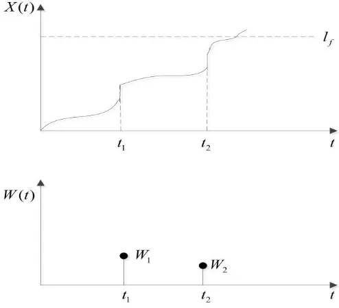
Figure 1 describes the degradation process of a system subject to external shocks. As shown in
the figure, shocks with magnitudes W1 and W2 arrive at times t1 and t2. The arrival of a shock
abruptly changes the degradation level. The system degrades continuously and fails when the
degradation level hits the threshold, lf. The failure threshold lf denotes the degradation level
where the mission cannot be satisfactorily performed. The threshold is usually determined by
engineers or experts. The overall degradation of the system can then be expressed as
( )
0 0
1
( , )= ( ) ( ) ( )
N t
i i
X t x D t W t x t B t W
(3)At the beginning of a PM cycle, the initial system state varies as imperfect PM actions are
carried out. While analyzing system reliability within a PM cycle, it is important to consider the
influence of initial state x0 and time t. Considering the arrival of random shocks, the reliability
of the system is expressed as
0 0
0
2 2
0
( , ) ( ) | ( ) ( )
( ) ( )
!
f k
t k
f w
k w
R t x P X t l N t k P N t k
l x t k e t
k t k
(4)7
Figure 1 Degradation processes subject to external shocks.
3.
Maintenance model for mission-oriented system
Three types of maintenance actions are considered in this paper: imperfect PM, preventive
replacement and corrective replacement. In practice, imperfect PM can refer to a simple repair,
oiling, cleaning, etc., which does not restore the system to being “as good as new”. Preventive
replacement can be an overhaul of the total system while corrective replacement can be a
physical replacement of the whole system (Peng et al., 2012; Chen et al., 2013). Although both
preventive replacement and corrective replacement can restore the system to the as-good-as-new
state, their contexts differ in practice. Corrective replacement is usually unplanned and
undertaken whenever the system is either in a state of severe deterioration or total failure (Huynh
et al., 2012; (Zhang et al., 2014).). An imperfect PM is carried out each time the overall
degradation level exceeds la. If the imperfect PM is unable to satisfy the prescribed reliability constraint, a preventive replacement is performed instead.
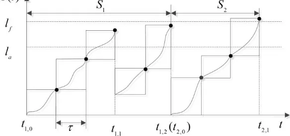
The PM process and system state evolution are shown in Figure 2. A renewal cycle is defined
as the time interval between two consecutive replacements (either preventive replacement or
corrective replacement). A PM cycle is defined as the time interval between two consecutive PM
actions or that between PM action and replacement (either preventive or corrective). Let Sm be
8
action in the mth renewal cycle. Note that, as we assume that each maintenance action is
instantaneous, the timing of the last maintenance action is identical with that at the beginning of
[image:8.612.162.454.146.283.2]the next PM cycle.
Figure 2 Description of PM process.
3.1 Improvement factor model
The improvement factor model is used to measure the restoration effect of imperfect
maintenance (Canfield, 1986). Wang and Pham (2011) utilized an improvement factor that scales
improvements in the failure threshold. Power-law relationship was constructed to characterize
the influence of the number of maintenance actions on the failure threshold. In this study, we
borrow the idea of power-law from Wang and Pham (2011) to measure the effect of imperfect
maintenance on system state.
In practice, the capacity of PM activity to improve system health weakens when more and
more PM actions have been taken. Moreover, unduly frequent disassembly and assembly can
even result in rapid degradation. Considering the above two aspects, the improvement factor
model is expressed as
*
( ) (1 i) f
X t l (5)
where X t( )* is the state of the system after PM , is the imperfect PM factor and i denotes the
index of PM action.
As the restored system state equals the starting state of the next PM cycle, for notational
simplicity, we denote 1
0 (1 )
i i
f
x l as the initial state of the ith PM cycle.
9
Preventive replacement is carried out at the end of the mission when the reliability of
completing the next mission reaches an unacceptable level, . The system reliability at the end
of the jth mission in the ith PM cycle can be obtained as
0
0 2 2
0
( ) ( )
( , )
!
i j k
f w
i
k
w
l x j k e j
R j x
k
j k
(6)Reliability constraint is essential for system operation, especially for safety-critical systems
such as high-speed railway and nuclear power plant (Liu et al., 2014).
Proposition 1. For system subject to Wiener degradation with linear drift and cumulative random shocks arriving according to a homogeneous Poisson process, system reliability of
completing missions decreases with the number of PM cycles.
Detailed proof is shown in Appendix A. Proposition 1 implies that there is a one-to-one
correspondence between the initial system state and the reliability of completing the next mission.
Therefore, the threshold for the reliability constraint, , can be transformed into the threshold of
the initial state, x0*, by using the following expression:
* 0
* *
0 arg max ( , 0) x
x R x (7)
As is shown in Equation 6, system reliability function ( )R decreases monotonously with the
initial degradation state if no maintenance actions are performed. By use of the monotonicity
property, x can be obtained as: 0*
* * *
0 0| ( , 0)
x x R x (8)
Due to the complexity of system reliability function ( )R , *
0
x cannot be obtained analytically,
instead numerical method is used to compute *
0
x . Equation 8 is useful in practice since the
system state can be measured at inspection and engineers or managers can make maintenance
decisions by observing the system state directly.
Imperfect PM is carried out when the PM action is able to restore the system to a state belowx0*.
Combining this observation with the improvement factor model by Equation 5, we have
* 0
10 * 0
log 1
f
x U
l
(9)
Equation 9 can be applied to determine the renewal cycle: ending with a preventive
replacement or with a corrective replacement. If the number of PM actions reaches U , then
preventive replacement is implemented. Otherwise, the renewal cycle ends with corrective
replacement. It can be concluded that the maximum number of imperfect PM actions U shows a
non-increasing trend with respect to the reliability threshold .
Proposition 2. The maximum number of imperfect PM actions is non-increasing with respect to the reliability threshold.
Detailed proof is given in Appendix B. Proposition 2 indicates that less imperfect PM actions
are allowed if high reliability constraint is required.
4. Formulation of long-run cost rate
Cost rate over an infinite horizon is used as the criterion to assess the performance of the
proposed maintenance model. After replacement (either corrective or preventive), the system is
restored to the state “as good as new”, which constitute a renewal cycle (Liu et al., 2015).
According to the renewal reward theory, the long-run cost rate is given as (Grall et al., 2002)
[ ] ( ) lim ( )
[ ] a
t
E C
C l CR t
E T
(10)
where CR t( )is the cost rate over time period [0, ]t , C is the cost in a renewal cycle and T is the
length of a renewal cycle.
The cost items include inspection cost at each inspection time CI, imperfect PM cost CM,
preventive replacement cost CP, and corrective replacement cost CC (including the penalty cost
due to mission abandonment). The renewal cycle can be classified into two types: renewal cycle
ending with preventive replacement or with corrective replacement. The long-run cost rate can
then be expressed as
[ ] [ ]
( )
[ ]
F U
C P M M I I
a
C P C P C E N C E N
C l
E T
11
where PF is the probability that a renewal cycle ends with corrective replacement, PU is the
probability that a renewal cycle ends with preventive replacement, NM is the number of
imperfect PM actions in a renewal cycle and N is the number of inspections in a renewal cycle. I
4.1 Scenarios of maintenance actions
Evolution of the degradation process X t x is a renewal process with the regenerative times
, 0
by corrective replacement or preventive replacement. Before we proceed to derive the expression
of the cost items, we first need to investigate the scenarios of various maintenance actions at
inspection. Within the ith PM cycle, there are four scenarios at the jith inspection time:
(1) If the degradation level exceeds the failure threshold lf , then a corrective replacement is
performed. The probability for such an event is given as:
0
0
1 0 0
0 0 0
( | ) { ( , ) (( 1) , ) }
{ ( , ) (( 1) , ) } ( ; ( 1) , ) ( ; ) ( ; ( 1) )
a i a i f
i i
i i f i a
l
i i i
i i f x i
x l
l i
x
P j i P X j x l X j x l
P X j x X j x l x dF x j x
F x f x j dx
(12) where 2 2 0 ( ) ( ) ( ; ) ! f t k w f l k wx k l e
F x k k
( ; )f x t is the pdf of the degradation level X t x( , 0)xat time t. Mathematically,
2 0 2 2 2 2 0 ( )
1 ( )
( ; ) exp
2( ) !
2 ( )
t k
w
k w w
x t k x e t
f x t
t k k
t k
(2) If the degradation level satisfies ( , 0)
i
a f
l X j x l , given the number of PM cycles
exceeds the maximum number U, iU, then preventive replacement is implemented.
The probability of such an event is:
0 1
2( | ) { ( , 0) (( 1) , 0) | } ( ( ; ) ( ; )) ( ; ( 1) )
U a
a f
i i
i a i f i a
l
l l i
x
i
P j i P l X j x l X j x l
F
U
x F x f x j dx
12
(3) If the degradation level satisfies la X j( ,x0i)lf , given the number of PM cycles is less
than U, i U , then imperfect PM is implemented. The probability of such an event is as
follows:
0
3( | ) { ( , 0) (( 1) , 0) | } ( ( ; ) ( ; )) ( ; ( 1) )
a
i a f
i i
i a i f i a
l
l l i
x
P j i P l X j x l X j x l
F x F
i U
x f x j dx
(14)(4) If the degradation level is less than la, X j( ,x0i)la , then the system is left as it was. The probability of such an event is given as:
4 0
0
2 2
0
( | ) { ( , ) }
( ) ( )
!
i
i i a
i j k
a i w i
k i w
P j i P X j x l
l x j k e j
k
j k
(15)4.2 Maintenance cost and length of a renewal cycle
Based on how a renewal cycle ends, the system renewal cycle can be classified into two types:
renewal cycle ending with a corrective replacement and renewal cycle ending with a preventive
replacement. In the following, the cost model is formulated separately, based on the type of
renewal cycles.
Case 1: Renewal cycle ending with corrective replacement
Corrective replacement is carried out when the system has failed at inspection. Given the
number of PM cycles i and the number of inspections in each PM cycleNIk, we can have the
associated cost and length of a renewal cycle as
1 1
0
( ) ( 1)
i
i k
I I I M C
k
C C N N C i C
(16)and
1 1
0 i
k i
I I
k
T N N
(17)where 0
0
I
13
The expected cost can be obtained by considering all the possible combinations of the number
of PM cycles and the number of missions completed in each PM cycle. After some calculations,
the expected cost can be obtained as
1 (1) (1)
1 1 1
3 1 3 1
1 1 1 1 1
1 1 3 1 1 1 1 3 1 1 1 [ ] [ ] [ ] ( | ) ( | ) ( | ) ( | )
( 1) ( | ) ( | )
( | ) ( | )
k i k i
k i
k i
F
I I M M
i
U i
I k k i i i i
i k j j k j j
i U
M i i
i k j j
i U
i i
i k j j
E C C E N C E N CcP
C j P j k j P j i P j i P j i
C i P j i P j i
Cc P j i P j i
1
(18)The expected length is given as
1 1 1
1 (1) 3 1 3 1
1 1 1 1 1
[ ] [ ] ( | ) ( | ) ( | ) ( | )
k i k i
i
U i
I k k i i i i
i k j j k j j
E T E N j P j k j P j i P j i P j i
(19)Detailed derivations are provided in Appendix C.
Case 2: Renewal cycle ending with preventive replacement
Preventive replacement is carried out when imperfect PM cannot bring the system back to a
state under reliability constraint. Based on the previous discussions, the reliability constraint can
be transformed to the limit of number of imperfect PM actions in a renewal cycle. The
preventive replacement is carried out at the end of a mission if the number of imperfect PM
actions reaches U , i.e., the system has survived the previous U PM cycles.
Given the number of inspections in each PM cycle, the cost of a renewal cycle ending with
preventive replacement can be obtained as
1 2
1 U
i
I I M P
i
C C N C U C
and the length of the renewal cycle is
1 2 1 U i I i
T N
14 0
0
2 (2) (2)
1 1 1 1
1
[ ] [ ] [ ]
( ( ; ) ( ; )) ( ; ( 1) )
( ( ; ) ( ; )) ( ; ( 1) )
a
i a f i
a
i a f
U
I I M M P
U l
I i x l l i M P
i j
U l
l l i
x i
E C C E N C E N C P
C j F x F x f x j dx C U C
F x F x f x j dx
(20)and the expected length of a renewal cycle as
0 0 1 2 1 1 1
[ ] ( ( ; ) ( ; )) ( ; ( 1) )
( ( ; ) ( ; )) ( ; ( 1) )
a
i a f i
a
i a f
U l
i x l l i
i j
U l
l l i
x i
E T j F x F x f x j dx
F x F x f x j dx
(21)Detailed derivations of Equation 20 and 21 are given in Appendix D. Combining the results of
the two cases, the long-run cost rate Ccan be readily obtained.
Corollary 1. The optimal long run cost rate for mission-oriented system is larger than that without mission constraint.
Proof. The conclusion is intuitive. For general system without mission constraint, the optimal
long run cost rate C
I,la
is obtained by optimizing the preventive maintenance threshold la
and the inspection intervalI. When the length of mission deviates from I* ( *I), we can always have C
la* C
I*,la*
.5.
Maintenance optimization
The objective of the maintenance policy is to minimize the long-run cost rate C. The decision
variable is the optimal threshold for imperfect PM action la . According to the analyses in
Section 4, the optimization model is formulated as
1 2
1 2
[ ] [ ]
min ( )
[ ] [ ]
a
E C E C
C l
E T E T
Subject to 0 M a f N U l l
The first constraint indicates that the number of imperfect PM actions cannot exceed the
15
implies the domain of the PM threshold la. Analytical solution of the optimization model is
difficult to obtain owing to the complexity of the cost model. Hence we have to resort to
numerical methods. In particular, search algorithm combined with Monte Carlo simulation is
adopted to optimize laand C l( )a
. When the number of simulation histories N is large enough, l
the cost model given by Equation 10 can be expressed as (Huynh et al., 2012)
( ) ( )
1 1
( ) ( )
1 1
[ ] ( ) lim ( ) lim
[ ]
l l
N N
n n
n n
a t N N N
n n
n n
C C
E C
C l CR t
E T
T T
(22)where ( )n
C and ( )n
T are the maintenance cost and length of a renewal cycle in the nth simulation
history.
The optimal la can be obtained by minimizing the long-run cost rate, i.e.,
arg min ( ) | 0
a
a a a f
l
l C l l l (23)
The following algorithm is used to determine the optimal la by searching over the range of
0,lf.Algorithm 1: Optimization algorithm
Step 1: Compute the value of U from Equations 8 and 9.
Step 2: Start with a small value of la.
Step 3: Determine the long-run cost rate from Monte Carlo simulation: 3.1: Initialization: set C 0and T 0.
3.2: Generate a historical account of degradation and shocks to determine the overall
degradation level X t( ).
3.3: Calculate the length and cost of a renewal cycle, T( )n and C( )n , respectively (see algorithm 2 below).
3.4: ComputeC C C( )n , T T T( )n and C C T
.
3.5: If Cconverges, go to step 4; else, repeat 3.1-3.4.
Step 4: If la lf , increase lawith a small increment and go back to step 3; else, go to step 5.
16
The following algorithm is used to determine the values of T( )n and C( )n in a Monte Carlo simulation.
Algorithm 2: Computation of T( )n and C( )n in a Monte Carlo simulation
Start from i1 (the number of PM cycles)
Step 1: Initialization: Set NIi 0.
Start from j1 (the number of missions in the ith PM cycle)
Step 2: At the end of a mission, decide using the following logic:
If
, 0
i a
X j x l , do nothing, let j j 1andNIi NIi 1, and turn back to step 2; else, go to Step 3.
Step 3: if lf X j
,x0i
la, and(a) if i U , do imperfect PM, updatei i 1and x0i (1 i1)lf, and return to step 1.
(b) if iU, do preventive replacement, get
1 ( )
1 U
n k
I I M P
k
C C N C U C
and1 ( )
1 U
n k
I k
T N
,and jump to step 5.
Step 4: if the system has already failed,X j
,x0i
lf , do corrective replacement, get1 ( )
0
( ) ( 1)
i
n k
I I M C
k
C C j N C i C
and1 ( )
0 i
n k
I k
T N j
, and proceed to step 5.Step 5: Output T( )n and ( )n
C .
In the following, we will present a numerical example to illustrate the effectiveness of the
proposed maintenance policy.
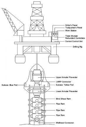
6. Application of subsea blowout preventer system
An example of subsea blowout preventer system is presented to illustrate the maintenance
procedure. Subsea blowout preventer system is used to seal, control and monitor oil and gas
wells to prevent blowout. It plays an important role in assuring safe working conditions for
deep-sea drilling activities. Failures of subsea blowout preventer system may lead to catastrophic
17
April 20, 2010 and oil contaminated wide area of seawater along the coast of Louisiana (Cai et
al., 2013). Thus high reliability has to be guaranteed during the operation of subsea blowout
preventer system. A subsea blowout preventer system is activated during deep-sea drilling. When
the drilling mission is completed, inspection has to be implemented to detect the health condition
of the system. During the drilling mission, the system is subject to internal degradation and
external shocks. A subsea blowout preventer system is mainly composed of blowout preventer
control system and blowout preventer stack, whose general structure is illustrated in Figure 3
[image:17.612.160.453.239.673.2](Cai et al., 2012).
18 6.1 Optimal maintenance policy
Suppose that the subsea blowout preventer system suffers a Wiener degradation process, with
the drift coefficient 0.2 and diffusion coefficient 0.02. The initial degradation level is 0.
The system is exposed to external shocks arriving according to a Poisson Process with the arrival
rate 0.5. The magnitude of each shock follows a normal distribution with w 0.1 and
0.01
w
.
Suppose further that the duration of a mission 3 months. After each mission, inspection is
carried out with the cost CI 1 (k$). After inspection, if the degradation level hits a prescribed
threshold la, an imperfect PM is carried out, with cost CM 10(k$). The imperfect PM exerts an
influence on the system state according to the improvement factor model (see Equation 5). The
improvement factor 0.6. A preventive replacement is carried out at the end of a mission if
the reliability of completing the next mission, 0.95, cannot be sustained. The cost associated
with the preventive replacement is CP 40(k$).
According to Equation 8 and 9, the maximum number of imperfect PM actions U in a renewal
cycle is computed as U = 4. If the overall degradation level of the system exceeds lf 8, the
system is deemed to have failed and corrective replacement is performed, with cost CC 80(k$).
The cost parameters are shown here for illustration purpose. In the following, the unit will be
suppressed for notational simplicity.
For imperfect PM, the influence of PM action decreases with the increasing PM cycles. Note
that the restored system state decreases rapidly with the increase of PM cycles. If the system
cannot be restored to a state satisfying the reliability constraint, preventive replacement has to be
performed. This implies a limited number of PM cycles within a renewal cycle.
We set the initial PM threshold as la 5 and search the optimal PM threshold la within the range [5, 8]. The step size is 0.02 and the number of repetitions for Monte Carlo simulation is
10,000. The goal of the maintenance policy is to find the optimal threshold for imperfect PM so
as to minimize the long-run cost rate. We obtain the minimum long-run cost rate of
1.5476
C at la 7.14. Figure 4 shows variation of the long-run cost rate C l( )a as a
19
optimal PM threshold la vary with the number of repetitions. The result shows that optimal C
and la converge when the number of repetitions Nl is larger than 500.
6.5 6.6 6.7 6.8 6.9 7 7.1 7.2 7.3 7.4 7.5
1.5 1.6 1.7 1.8 1.9 2 2.1 2.2 2.3 2.4
PM threshold la
L
o
n
g
-r
u
n
co
st
r
a
te
[image:19.612.112.500.138.358.2](7.14,1.5476)
Figure 4 Long-run cost rate vs PM threshold.
Table 1 Optimal decisions vs number of repetitions
Number of repetitions Nl Minimum long-run cost rate C Optimal PM threshold la
50 1.5455 7.22
100 1.5458 7.20
500 1.5486 7.14
1,000 1.5469 7.14
5,000 1.5473 7.14
10,000 1.5476 7.14
The system deteriorates by natural degradation and external shocks, and improves following
maintenance actions. It is therefore of interest to investigate the variation of system reliability as
a result of the degradation (external shocks) and maintenance actions. Figure 5 shows the system
reliability within a renewal cycle. Note that system reliability has been restored to 1 at times 30,
[image:19.612.87.524.430.588.2]20
corresponding PM actions are carried out at these time points. Also note that the reliability of the
system is different when maintenance actions are carried out at times 30, 48, 57 and 63.This is
due to the mission constraint that inspection and imperfect PM can only be performed at the end
of a mission. This is different from systems where maintenance actions can be carried out at any
time. Note also that, due to the uncertainty of Wiener process and randomness of external shocks,
the number of imperfect PM cycles and maintenance times can vary from one renewal cycle to
another. For illustration purposes, we only depict the variation of system reliability in a renewal
cycle in the case that the renewal cycle ends with a preventive replacement.
0 10 20 30 40 50 60 70
0.82 0.84 0.86 0.88 0.9 0.92 0.94 0.96 0.98 1
Time t
re
lia
b
ili
ty
R
(t
[image:20.612.103.503.251.461.2])
Figure 5 Variation in system reliability over time.
6.2 Sensitivity analysis
Sensitivity analysis is performed to examine the uncertainty of the optimal maintenance policy.
The parameters of interest are the length of the mission , the imperfect PM factor , and the
arrival rate of the Poisson process . In the following, we investigate the influence of the three
parameters on the optimum PM threshold. The results shown in Figures 6 to 8 are obtained by
varying one parameter at a time while fixing the other parameters.
Figure 6 shows the variation of Cwhen is increased progressively from 2 to 4. Note that,
when 4 , the corresponding optimal PM threshold la 6.5; when 2 or 3 , the
21
maintenance policy is based, the results imply that the optimal maintenance policy is affected by
the mission length . Also note that, when changes from 2 to 4, the corresponding optimal
long-run cost rate C, decreases from 1.8565 to 1.5, which indicates a decreasing trend with .
Actually, the impact of on the long-run cost rate is two-fold. A larger value of requires lesser inspection within a renewal cycle; thus incurring a lower inspection cost. Meanwhile, a
greater penalty cost is incurred if the mission constraint prevents an appropriate maintenance
action from being taken in a timely manner. The results shown in Figure 6 verify this. As we can
see, when lais smaller than the optimal value, the long-run cost rate decreases with . This is because when the PM threshold is low, the system needs to be maintained more frequently, so
the impact of mission constraint on the maintenance cost rate is not as significant as that with the
inspection number. However, when lais large, the impacts of mission constraint and inspection
number become intricate.
5 5.5 6 6.5 7 7.5 8
1.5 2 2.5 3
PM Threshold l
a
E
xp
e
ct
e
d
C
o
st
R
a
te
=2
=3
[image:21.612.110.499.340.551.2]=4
Figure 6 Sensitivity analysis of on the long-run cost rate.
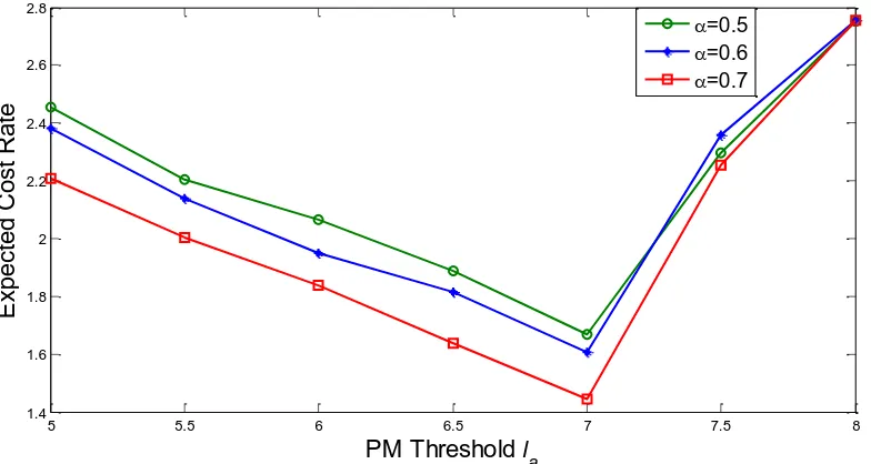
As shown in Figure 7, when the imperfect PM factor increases from 0.5 to 0.7, the
minimum long-run cost rate decreases from 1.6692 to 1.4484. When the PM threshold is small (≤
7), the long-run cost rate shows an obviously decreasing trend with increasing . However, the
trend is not so obvious when labecomes quite large. This is due to the fact that, when la is larger,
22
turns out to be less significant. It is interesting to note that when laapproacheslf, the long-run cost rate remains constant. This can be explained by the fact that when the PM threshold is equal
tolf, the imperfect maintenance policy is reduced to a block replacement policy (Beichelt, 1981),
which is irrelevant to . Also note that although the long-run cost rate varies with , the PM threshold lato achieve the minimum cost rate remains invariant. This implies that the optimal maintenance policy is not sensitive to the imperfect PM factor.
5 5.5 6 6.5 7 7.5 8
1.4 1.6 1.8 2 2.2 2.4 2.6 2.8
PM Threshold l
a
E
xp
e
ct
e
d
C
o
st
R
a
te
=0.5
=0.6
[image:22.612.110.502.242.451.2]=0.7
Figure 7 Sensitivity analysis of on long-run cost rate
The arrival rate influences the maintenance policy and the maintenance cost rate in a way
that an increase in accelerates the overall degradation level of the system. As a result, more
frequent maintenance actions are required to keep the system operating. Not surprisingly, the
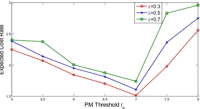
long-run cost rate increases as increases. As shown in Figure 8, when increases from 0.3 to
0.7, the minimum long-run cost rate increases from 1.5094 to 1.7433. This points to an
increasing trend of long-run cost rate with increasing . Similar to the results shown in Figure 6,
the optimal maintenance policy is insensitive to the arrival rate . This demonstrates the
23
5 5.5 6 6.5 7 7.5 8
1.5 2 2.5 3
PM Threshold la
E
xp
e
ct
e
d
C
o
st
R
a
te
=0.3
=0.5
[image:23.612.110.499.84.296.2]=0.7
Figure 8 Sensitivity analysis of on long-run cost rate.
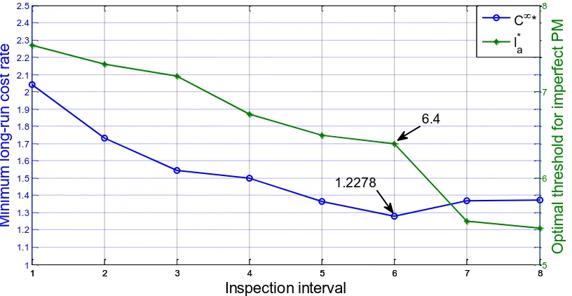
6.3 Comparison with general system
In order to investigate the effect of mission constraint on maintenance policy, a comparison
study is conducted for a general system without mission constraint. The general system for
comparison is a continuously operating system subject to natural degradation and external shocks.
Yet inspection can be carried out at arbitrary time. Reliability constraint is interpreted as to
ensure that the system operates above reliability threshold until next inspection. The objective of
the maintenance policy is to determine the inspection interval I and threshold for imperfect PM
a
l , so as to minimize the long-run cost rate C(I, )la . The cost parameters and degradation parameters are identical as previously shown. Figure 9 plots the variation of long-run cost rate
and optimal threshold for imperfect PM with the inspection interval. The optimal maintenance
policy for a general system is obtained at I*6 , la* 6.4 , with the minimal cost rate
*
1.2278
C . Compared with mission-oriented system, maintenance decision for general system
24
1 2 3 4 5 6 7 8
1 1.1 1.2 1.3 1.4 1.5 1.6 1.7 1.8 1.9 2 2.1 2.2 2.3 2.4 2.5
M
in
im
u
m
l
o
n
g
-r
u
n
co
st
r
a
te
Inspection interval
1 2 3 4 5 6 7 85
6 7 8
O
p
ti
m
a
l
th
re
sh
o
ld
f
o
r
im
p
e
rf
e
ct
P
M
C*
l*
a
1.2278
[image:24.612.110.518.85.296.2]6.4
Figure 9 Optimal PM threshold & cost rate for a general system.
7. Conclusions
An imperfect maintenance policy is developed in this paper for mission-oriented systems
subject to degradation and external shocks. The reliability of the system is derived using a
cumulative shock model depicting the influence of external shocks on the system’s degradation
level. Both reliability and mission time constraints are taken into account while formulating the
maintenance policy. Cost model is developed by classifying a renewal cycle into two types:
ending with preventive replacement and with corrective replacement. Optimal solution is
obtained by minimizing the long-run maintenance cost rate. Results from a numerical example
show that the optimal PM threshold is significantly affected by the length of the mission, thus
confirming the importance of mission time constraint and verifying the effectiveness and
significance of the proposed maintenance model for mission-oriented systems.
Further advances can be achieved by relaxing some assumptions made in this paper. For
example, imperfect inspection can be taken into consideration, as in reality, the true system state
is almost impossible to obtain due to the existence of noise or limitations related to inspection
techniques. Another possible improvement relates to the improvement factor model used in this
25
addition, one can further investigate the influence of length of a mission on the maintenance
policy.
Acknowledgements
The work described in this paper is partly supported by a grant from City University of Hong
Kong (Project No.9380058) and also by National Natural Science Foundation of China (No.
71371163).
Appendix A
Proof of Proposition 1.
Equation 6 shows the system reliability of completing j missions. By taking derivative with
respect to x0i, we have
0
0 0
2 2 2 2
0 0
( )
( , ) ( )
0 !
i
i k i
f w
i
k w w
l x j k
R j x e x
x k k k
which indicates that system reliabilityR j x( , 0i) is a decreasing function with respect to the initial degradation levelx0i.
From Equation 5, we have
1 0 (1 )
i i
f
x l
which implies that x0i increases monotonically with the number of PM cycles i. Hence, it can be
readily concluded that R j x( , 0i) decreases with the number of PM cycles i.
Appendix B
Proof of Proposition 2.
Denote g( , x0*, ) R( , x0*) . As is a constant here, it can be obtained that
* *
0 0
* *
0 0
1 1 0
/
x x
g g
x g x
Since * * *
0 0 0
/ ( , ) / 0
g x R x x
26
we have x*0/ 0, which implies that the threshold of the initial state x*0 decreases with respect to the reliability threshold .
As 1, with Equation 9, it can be obtained that U is non-decreasing with x . Therefore, it 0*
can be concluded that the maximum number of imperfect PM actions U is non-increasing with
respect to the reliability threshold .
Appendix C
Derivations of Equation 18 and 19.
Assume that there are i (i U ) PM cycles before corrective replacement in a renewal cycle.
1( i| )
P j i denotes the probability that a failure occurs after completing ji missions, given that a
failure has occurred in the ith PM cycle. In the ith PM cycle, the probability that the renewal
cycle ends with a corrective replacement can be obtained as
1 1 0 1 1 1 11 0 1 0
0 0
1
3 1
1
( ) ( , 0) (( 1) , 0)
( , ) (( 1) , )
( , ) (( 1) , )
( | ) ( | )
( ( ; ) ( ; )) ( ; ( 1) )
i i
k i
a
k a f
F
f a a
j
i i
f i a i a
j
i i
i f i a
j i i i j j k l
l l k
x
P i P l X j l X j l
P l X j x l X j x l
P X j x l X j x l
P j i P j i
F x F x f x j d
0 1 1( ; ) ( ; ( 1) )
k a i f i i j k l l i x j x
F x f x j dx
The probability that the renewal cycle ends with a corrective replacement can then be obtained
by summing all the F( )
P i for i1, 2...,U1. Mathematically,
0
0
1
1 1
1 1 1
( ) ( ( ; ) ( ; )) ( ; ( 1) )
( ; ) ( ; ( 1) )
a
k a f k
a i f i
i
U U l
F F
l l k
x
i i k j
l
l i
x j
P P i F x F x f x j dx
F x f x j dx
27 0 0 1 (1) 1 1 1 1 1
[ ] ( 1) ( )
( 1) ( ( ; ) ( ; )) ( ; ( 1) )
( ; ) ( ; ( 1) )
a
k a f k a i f i U F M i i U l
l l k
x
i k j
l
l i
x j
E N i P i
i F x F x f x j dx
F x f x j dx
To compute the number of inspections in a renewal cycle NI(1), we first need to determine the
number of completed missions ji in the ith PM cycle. Given that the system fails in the ith PM
cycle, we can have the conditional expected number of inspections as
1
| (1) 3 1
1 1 1 1
[ ] [ ] ( | ) ( | )
k i
i i
k
i I I k k i i
k k j j
E N E N j P j k j P j i
The expectation of NI(1) can be computed by considering all the possible realizations of the number of PM cycles, which is expressed as
0
0 1
(1) | (1) 1
1 1
3 1
1 1 1 1
1 1 1 1 1
1
[ ] [ ] ( )
[ ( | ) ( | )] ( )
{[ ( ( ; ) ( ; )) ( ; ( 1) )
( ; ) ( ; ( 1) ) ]
( (
k i
a
k a f k a i f i a U F
I i I
i
U i
F
k k i i
i k j j
U i l
k x l l k
i k j
l
i x l i
j
l
E N E N P i
j P j k j P j i P i
j F x F x f x j dx
j F x f x j dx
F
0 0 1 1; ) ( ; )) ( ; ( 1) )
( ; ) ( ; ( 1) ) }
a k f k a i f i i l l k x j k l l i x j
x F x f x j dx
F x f x j dx
28 0
0
0
0
1 (1) (1)
1 1 1 1 1
1 1 1
[ ] [ ] [ ]
{[ ( ( ; ) ( ; )) ( ; ( 1) )
( ; ) ( ; ( 1) ) ]
( ( ; ) ( ; )) ( ; ( 1) )
(
a
k a f k
a i f i
a
k a f k
a i f
F
I I M M
U i l
I k x l l k
i k j
l
i x l i
j
i l
l l k
x j k l l x
E C C E N C E N CcP
C j F x F x f x j dx
j F x f x j dx
F x F x f x j dx
F
0 0 0 0 1 1 1 1 1 1 1 1; ) ( ; ( 1) ) }
( 1) ( ( ; ) ( ; )) ( ; ( 1) )
( ; ) ( ; ( 1) )
( ( ; ) ( ; )) ( ; ( 1) )
( ; ) (
i
a
k a f k
a i f i
a
k a f k a i f i j i U l
M x l l k
i k j
l l i x j i U l
l l k
x
i k j
l l x
x f x j dx
C i F x F x f x j dx
F x f x j dx
Cc F x F x f x j dx
F x f x
; ( 1) )i
i j
j dx
and the expected length of a renewal cycle is
0 0 0 0 1 1 1
1 1 1
1 1
1
[ ] {[ ( ( ; ) ( ; )) ( ; ( 1) )
( ; ) ( ; ( 1) ) ]
( ( ; ) ( ; )) ( ; ( 1) )
( ; ) ( ; ( 1) ) }
a
k a f k
a i f i
a
k a f k
a i f i
U i l
k x l l k
i k j
l
i x l i
j
i l
l l k
x j k l l i x j
E T j F x F x f x j dx
j F x f x j dx
F x F x f x j dx
F x f x j dx
Appendix D
Derivations of Equation 20 and 21.
The probability for occurrence of preventive replacement is given as
0 1 0 0 1 1 0 1( , ) (( 1) , )
( ( ; ) ( ; )) ( ; ( 1) ) ( 1) ,
a
i a f a
U
U i i
f i a i a
i
U l
l l i l
i i
x i
P P l X j x l X j x l
F x F x f x j dx F j x