Syed. M. Z. Abbas Shah*, S. Marshall and P. Murray
*Department of Electronics Engineering, Mehran University of Engineering and Technology, Jamshoro, Sindh, Pakistan
Email: [email protected] , Tel: +92-222-2771334
Department of Electronic and Electrical Engineering, University of Strathclyde, Glasgow, United Kingdom
Abstract. The presence of specular highlights can hide underlying features of a scene within an image and can be problematic in many application scenarios. In particular, this poses a significant challenge for applications where image stitching is used to create a single static image of a scene from inspection footage of pipes, gas tubes, train tracks and concrete structures. Furthermore, they can hide small defects in the images causing them to be missed during inspection. We present a method which exploits additional information in neighbouring frames from video footage to reduce specularity from each frame. The technique first automatically determines frames which contain overlapping regions before the relationship that exists between them is exploited in order to suppress the effects of specular reflections. This results in an image that is free from specular highlights provided there is at least one frame present in the sequence where a given pixel is present in a diffuse form. The method is shown to work well on greyscale as well as colour images and effectively reduces specularity and significantly improves the quality of the stitched image, even in the presence of noise. While applied to the challenge of reducing specularity in inspection videos, the method improves upon the state-of-the-art in specularity removal, and, its applications are wide-ranging as a general purpose pre-processing tool.
Keywords Image Projection, Specular Reflection Removal, Visual Inspection, Non-Destructive Evaluation
1. Introduction
Automated Non-Destructive Evaluation (NDE) using visual inspection was studied by [1] and finds applications in pipe inspection [2], train track inspection [3] and inspection of concrete structures [4]. The process usually employs a camera mounted on a mobile robot, automated vehicle or other apparatus which is moved over an area to be inspected while images are captured in quick succession. These images can then be analysed locally or offline so as to assess the condition of the structure being inspected. During offline processing, the images captured can be stitched together to provide a seamless view of the inspected surface [5-9]. However, due to the use of light
sources for illuminating the scene to be captured and sources present in the environment, specular reflections can appear in these images and this can reduce the accuracy of image alignment methods used prior to image stitching [1]. Furthermore, for the purposes of visual inspection, the presence of specularities could also lead to defects being missed during the inspection process or spurious false defects being detected. It is anticipated that if such images can be pre-processed to reduce specular highlights, they can be more easily and more accurately stitched together to provide a high quality specular free view of the inspected area in full, thereby making manual or automated monitoring more robust. It is therefore necessary that suitable techniques be developed for the
removal of specular highlights which motivates this work.
The paper is organised as follows, Section 2 provides a description of the current state-of-the art techniques for specularitiy removal and motivates the case for the proposed approach. In Section 3 we present the proposed technique for specularity removal and we provide a number of examples to aid the understanding of its description. The results of applying the proposed approach and alternative techniques to various datasets are discussed in Section 4 and, in Section 5, we give some concluding remarks.
2. Related work
The detection and removal of specular reflections from images has been an area of interest to the Computer Vision community for many years, and existing techniques for this task find applications in medical science [10-12], video surveillance [13], image refinement and image reconstruction [15-17]. Citing the importance of the availability of such methods, there have been various attempts to address this issue.
2.1. Single Image methods
A number of authors have provided methods using a variety of approaches to remove specular highlights using synthetically generated specular free images [18-23]. The authors use a number of sophisticated techniques to reduce specularities and they present very good results but each has some drawbacks. The authors in [23] propose a speeded up version of the method of [18] by replacing their proposed iterative method with a bilateral edge preserving filter to improve speed. The methods from [18-23] all use a synthetically constructed ‘specular free’ image which requires that the surface colour is chromatic and that diffuse pixels are present for every colour region. An inpainting technique is proposed in [22] while using a specular free image, this however, does not recover any
abnormalities hidden by specular highlights as the inpainting is carried out using non-specular neighbouring pixel values. The authors in [24] presented a method that uses averaging to remove specularity from data used for image based dietary assessment. The method works well for the author’s application. However, since the approach relies on averaging, features in the final result can appear blurred and distorted. Another approach in [25] rearranges the chromaticity distribution between specular and diffuse pixels to remove highlights while smoothing this distribution using achromatic components of the diffuse pixels. All these methods require the presence of colour content in the images.
2.2. Multi-image methods
requirements on the type of imaging equipment that is required.
As discussed, there are a large number of techniques which can be used to suppress specularities in image data. However, many of the available techniques can only be applied to colour images which contain distinctive chromaticity [18-23, 26]. This is not suitable for visual inspection applications where data can be greyscale or single-colour. Furthermore, many techniques operate on a single image basis whereas, when processing video data it makes sense to utilise information from overlapping frames and exploit the motion of specularities in order to remove them from the video data. While three techniques which exploit this property are discussed in [26-28], all three methods require a very specific capturing environment or capture device to be used. They also assume that the alignment between overlapping images is known and constant and, in the case of [26], the approach can only be applied to colour images. Clearly a technique which can be applied to both grey and distinctive colour images captured using any single camera and light source would be highly beneficial for a wide range of applications.
In this paper, we present a simple yet innovative software based technique to remove specular highlights from a sequence of images. The method requires a single (non-specific) camera and illumination source and, unlike the approaches in [20-23, 28], can be applied to both colour and greyscale data without modification which makes greatly improves its applicability in a number of application areas. We exploit the fact that the content of images in a sequence captured by a moving camera will overlap each other to some extent, and we use this to compute the relationship between such images directly from the data itself. This alleviates the need for multiple cameras to remain at a fixed position during image acquisition [26,27] which is impractical for many applications. While for most inspection videos the camera is moved around a scene to be imaged, the proposed method would work equally well if applied using a
fixed camera and a moving scene e.g. for inspecting parts on a conveyor belt.
Furthermore, the proposed approach is software based and performs equally well on both colour and greyscale images and, in Section 5, it is shown that it also produces significantly better results than that of [24] when applied to the same set of image data. We consider [24] for comparison since it proposes an application environment without constraints (no restrictions on capturing images) or content (colour or grey) of the images being captured.
3. Specularity Removal Using Image Correspondences
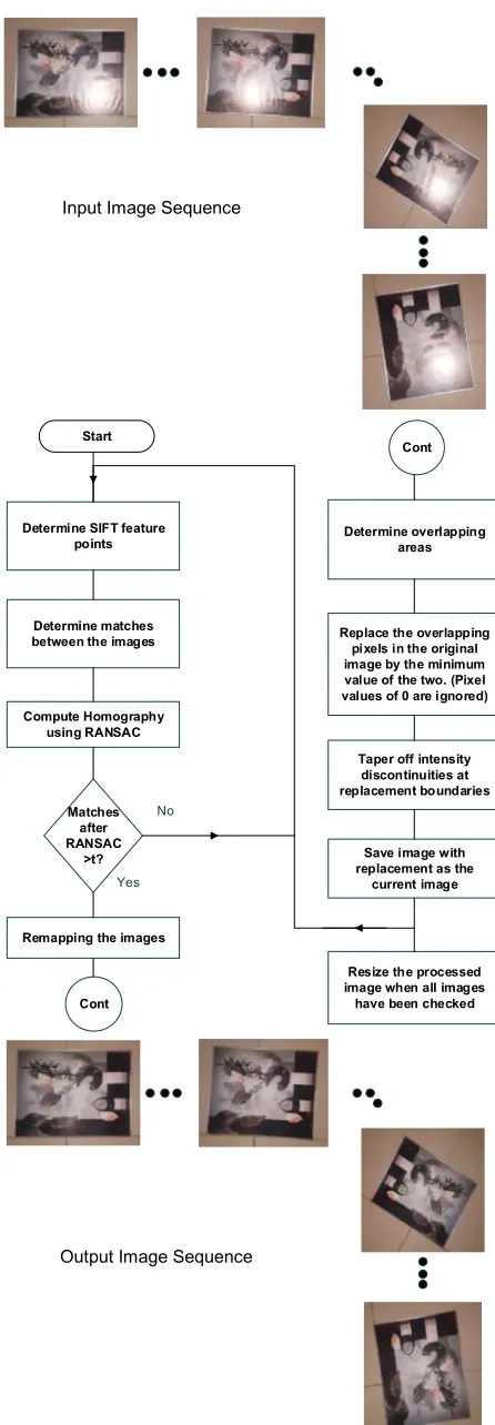
The procedure used for the reduction of specularity from the images is illustrated in the flowchart shown in Fig. 1. The method requires multiple images of the same scene from different vantage points, ideally successive frames from a video work well as an input to the process. Specular highlights are removed from the frames using a seven step process taking a single image at a time for specular highlight removal.
3.1. Determination of feature points
Determine SIFT feature points
Determine matches between the images
Compute Homography using RANSAC
Matches after RANSAC
>t?
Remapping the images
Determine overlapping areas
Taper off intensity discontinuities at replacement boundaries Replace the overlapping pixels in the original image by the minimum value of the two. (Pixel values of 0 are ignored)
No
Yes
Cont
Cont
Resize the processed image when all images have been checked
Save image with replacement as the
current image Start
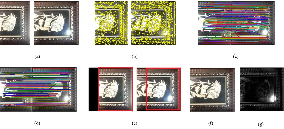
by a descriptor which can be used to identify each point. As a demonstration, consider the images shown in Fig. 2(a). Fig. 2(b) shows the SIFT feature points extracted from these two images. Each of the yellow circles indicates a feature point, the radius of the circle indicates the scale at which the feature point exists and the line within the circle indicates its orientation.
3.2. Determination of matching points and image alignment
Once the feature points have been determined, the next step is to search for possible matches. The matching of SIFT key points is accomplished by computing the Euclidean distance among the descriptors between any two points in two different images. If, for any feature point in any image, two points are found in the other image whose ratio of the distance from the considered point is greater than or equal to 0.8 [39], both the points are dropped as potential matches. This was found the authors in [39] to reduce false match detection by 90%. A k-d tree [40] is used to find the neighbourhood in which matching is to be carried out to reduce matching time.
Aligning matching images requires that both the images are projected onto the same plane. The motion between the images can take an arbitrary direction and rotation and nonlinear effects may also be present due to the change of plane and view of the capturing apparatus. This motion can be mathematically modelled as perspective motion between the two images. The relation between the pixels in two images can be mathematically described by means of a Homography matrix, H
computed between the two images, it is given as shown in (1).
=
ℎ ℎ ℎ
ℎ ℎ ℎ
ℎ ℎ ℎ
(1)
Input Image Sequence
Output Image Sequence
[image:4.612.80.303.65.707.2]where the elements ℎ are arbitrary numbers that define the transformation. The homography is computed using RAndom SAmple Consensus (RANSAC) [41] together with the Direct Linear Transformation (DLT) [42]. The probability that a correct model has been identified using RANSAC is given by (2)
= 1 − (1 − ) (2)
Where pgt is the probability of the determined geometric model being correct, p is the probability that the considered point is a legitimate candidate for the geometric model to be determined (Inlier), m
is the number of points used for determining the geometric model and k is the number of trials the algorithm iterates through. The number of trials
used for RANSAC is k=100 (empirically
determined to be sufficient to generate a dependable homography, increasing the number of trials didn’t have a significant impact in a correct homography being determined) and the number of points used in each trial is m=4 (in the DLT, 4 points are enough to compute 2D Homograpy [39]). It is importantto ensure that a photographically correct homography is determined between two images.That is, a homography is considered valid if and only if there is an actual overlap between the images and not valid if it is computed usingerroneously matched points. We achieve this by applying a threshold
t=28 to the number of inliers found to decide whether the computed homography is the result of falsely matched points or otherwise. A similar approach has been used in [39]. The threshold value of 28 can be adjusted by the user as an additional input to the algorithm and has been determined empirically by visual inspection of homographic transformation matrices computed for 158 different images. The matching points between the images before and after RANSAC are shown in Fig. 2(c) and Fig. 2(d) respectively. By observing that the points in Fig. 2(d) appear to be separated by some fixed distance and orientation, it is clear that the removal of outliers has been successful.
3.3. Remapping of the Images
After the determination of an appropriate geometric transformation between the images, the next step is to realign them. Using only the homography between the images results in an alignment error due to measurement inaccuracies and inclusion of erroneous points that fall within the chosen RANSAC threshold. In order to overcome this, the images are aligned by warping both the images separately on to two identical environment maps
formed using the calculated projective
transformation matrix. The meshes are created in the Cartesian coordinate system to avoid any change of shape in the original images which may result from using either Cylindrical or Spherical coordinate systems. The compositing surface in Cartesian coordinates was created as in (3)
= 11 ,1 2 ,, 22 1, 2
1 1 1 1
(3)
Where col,im2,row,im2 represent the column and the row size of the matched image and Cmat is the compositing matrix. The new pixel locations for each original pixel in the environment map is then calculated as in (4) and (5).
=(ℎ
∗+ ℎ ∗+ ℎ )
ℎ ∗+ ℎ ∗+ ℎ (4)
=(ℎ
∗+ ℎ ∗+ ℎ )
ℎ ∗+ ℎ ∗+ ℎ (5)
3.4. Determination of overlap between the Images
Since the images have been aligned properly due to the warping of both the images, the original image is searched for in its environment map and the same pixel locations are extracted from the environment map of the second image. The second extracted image will have a portion which overlaps the first image and a portion which does not contain useful data. This is due to the partial overlap between the two images because of the motion within any input video or series of images. The overlapping area in the two images in Fig. 2(e) is marked by a red boundary.
3.5. Replacement of pixels for specularity reduction
Since specular points are characterized by high pixel values and diffuse pixels are characterized by low values, the pixels in the overlapping region are replaced by the minimum of the values in the two images as given in (6).
( )= min _ , _ (6)
where ( ) is the overlapping region of
the two images in which pixels have been replaced
by their diffuse counterparts, _ and
_ are the overlapping parts between the first
and the matched image. This results in the replacement of all pixel values in the original image by the minimum value of the two. The original image after specular reduction has been applied is shown in Fig. 2(f). It can be observed that replacement by the minimum value of the overlapping pixels has reduced specular highlights significantly since diffuse values for corresponding pixels were present in the other images.
3.6. Smoothing of intensity discontinuities in the Image
Due to vignetting (the decline of intensity towards the edges) and non-uniform illumination, an intensity discontinuity may appear at the boundaries of overlapping regions between the images when pixels are replaced by the minimum value. In order to overcome this artefact, smoothing can be employed to taper off the intensity discontinuities at the boundaries of overlapping images. A four step procedure is used to smooth out these discontinuities.
(i) The location of the edges of the overlapping regions between the images is first determined.
(ii) The presence of an intensity discontinuity is then detected by applying a threshold to the difference of the original and the processed image. The threshold is determined using the method presented in [43]. This results in a binary image which consists of bright values at all points where there is a difference of intensity between the original and the processed images.
(iii) Using the information from the computed homography between the images, the appropriate edge locations determined in step (i) are then used to search for a discontinuity (a bright value). If a bright value is detected, the intensity values in the processed image are smoothed off linearly in the direction of higher intensity. This smoothing of intensity is carried out over 10 pixels starting at the location of the discontinuity. A Gaussian function was also tested for this purpose but the results from the test were less convincing.
in the geometric transformation between the images and an incorrect feature alignment may result otherwise.
3.7. Resize processed image
In this step the processed image is resized to the original image size. Depending on the effect of warping on the final processed image, this may require a combination of decimation and interpolation.
For Fig. 2(f), since no discontinuity appears in the processed Portrait Image, no smoothing has been performed in the output image but it has been resized to the original image size. Fig. 2(g) shows the difference between the original image and the specular reduced image produced by the proposed method. It can be observed that specular highlights have been successfully removed.
4. Experimental results
In this section we present the results of applying the proposed technique to three different datasets. In order to demonstrate the efficacy of the proposed approach compared to the method of [24] as other methods require use of specialist hardware. Furthermore, the said approach is touted to not require any special capturing apparatus or content of the image captured which is similar to the aim of the work. In the first experiment, we use a dataset which consists of two images of a plate captured in a scenario similar to that described in [24]. The second dataset consists of inspection images of a metal sheet taken at a rate of 30Hz with two halogen lights as the light sources. These images are the same as those used in [1]. This set of images is grey with almost no chrominance measure and contains dispersive specular highlights. The third image set consist of images of a plate to demonstrate the algorithms operation for two types of surfaces, those having depth discontinuity and second, the presence of colour content. It is notable to point out that no special capturing equipment was used in the image
acquisition process as the image was captured using a Samsung Galaxy S6 back camera.
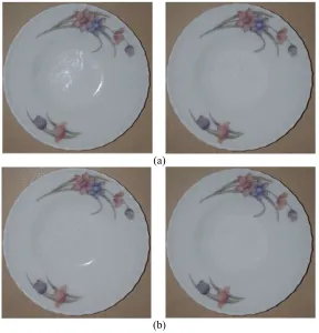
4.1. Comparison using plate images similar to images used in [24]
In order to demonstrate the effectiveness of the proposed method, we have applied and compared the method of [24] with the technique described in this paper using the images shown in Fig. 3. Fig. 3 also shows the processed images resulting from both algorithms. As can be observed from the figure, the specular highlights have significantly been reduced by the proposed algorithm as compared to the technique in [24]. It can be observed that the minimum function has resulted in most of the specular pixels being replaced by corresponding darker counterparts in the second image. As observed, this outperforms the averaging process being used for specularity reduction in the method of [24] as most of the speckle in both the images tested has been removed when applying our approach (Fig. 3 (b) compared to Fig. 3(a)).
4.2. Specular reduction in Colour images and perception of depth
observed which has been shown in Fig. 4(b). It can be seen that the output is free from specular reflections. Furthermore, the irregular patterns around the plates rim have also been preserved.
4.3. Specular reduction in Greyscale images
A two image subset of the last dataset for testing is shown in Fig. 5(a) and is used to demonstrate the proposed algorithm on greyscale images of aluminium sheets used in [1]. Due to lighting conditions and surface reflectivity, the authors of [1] were not able to use these images for image mosaicing purposes due to specular highlgihts. We have used a larger number of octaves (12) for each image which results in feature points being detected. This is an advantage of the SIFT algorithm in that one can tune the number of octaves to form the scale space in which features are searched for. Each image covers an area of 40 x 30 mm. Fig. 5 shows the original, specular reduced and the difference between the two images for the monitoring dataset to illustrate the amount of specular highlgihts that has been removed from the images . As can be seen from Fig. 5, the specular highlights have been completely removed in Fig. 5(b) (right) with partial removal being observed for Fig. 5(b) (left). This is due to the partial overlap occurring between it and the rest of the images in the set. One aspect of concern however is the presence of a discontinuity in the specular reduced image of Fig. 5(b) (left) and Fig. 5(b) (centre). This effect is mitigated by using linear tapering around the discontinuity edges, the result of which can be observed in Fig. 5(c) (left) and Fig. 5(c) (centre). The difference between the original and the specular reduced image is shown in Fig. 5(d). Fig. 5(d), points out the specular highlights which have been removed with this method.
4.4. Noise tests
In order to check the performance of the algorithm in presence of noise, three noise models were used
to corrupt the images with increasing levels of variance. The noise models used were
(i) Gaussian white noise (ii) Speckle noise
(iii) Salt and Pepper noise
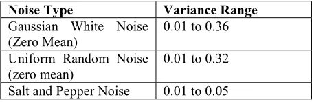
[image:8.612.313.540.300.374.2]Tests for noise were performed on three images taken from the Portrait dataset (used to explain the proposed method in Section 3) and have been shown in Fig. 6(a). The Peak Signal to Noise Ratio (PSNR) was used to indicate to the quality of the image. Table 1 shows the variances applied for each noise type before the algorithm was found to stop giving satisfactory results.
Table. 1 Summary noise types and variances for noise tests
Noise Type Variance Range
Gaussian White Noise
(Zero Mean) 0.01 to 0.36 Uniform Random Noise
(zero mean) 0.01 to 0.32 Salt and Pepper Noise 0.01 to 0.05
considers ‘pepper’ pixels to be diffuse. Of course, in practice a simple median filter could be used to pre-process the image prior to application of the proposed techniques to circumvent this issue.
In all three experiments with noise, there is an overall improvement in the PSNR of the processed images. In some cases, however, as present for the Uniform Random Noise and Salt and Pepper noise the PSNR does not improve or is less than the PSNR of the corrupted images.
Lastly, we applied median and average filters of window sizes of 3x3 up till 10x10 pixels to the images before the application of the algorithm. As expected, it was observed that averaging distorted the features in the images as well as spread the specular highlights. The averaging was carried out to check the effect of blur on the proposed scheme. The median filter was observed to remove noise well for low variance values but, as expected, its performance deteriorated with increasing amounts of noise. Additionally, corners and details such as edges were distorted. The algorithm did not give satisfactory results for filters of larger window sizes as it rendered distorted feature points unmatchable.
4.5. Translation and Rotation Tests
In order to test the algorithm for the limitation in terms of movement, the images were shifted using a translation function and the output was visually inspected. It was found that for the given image set the algorithm worked smoothly for a maximum translation of 200 pixels in both X and Y directions. This is due to the use of the Cartesian mesh on to which the images are warped which limits the amount of allowed motion between the frames. This is also important as it allows for a sparse image acquisition and processing.
To test the performance of the algorithm in the presence of rotations between images, tests were conducted by rotating the images by 15˚ each time and it was observed that the algorithm worked satisfactorily for all rotations.
5. Conclusion
In this paper, we present a method for the removal of specular highlights from a sequence of continuous images. It has been shown that detecting correspondences between successive images and calculating the geometric transformation between them, one can use information from neighbouring images to reduce/remove specular highlights from image sequences and video frames. The proposed method has been shown to work on greyscale as well as colour images which is a major advantage over previous work in this area. Being a software based approach, this method allows for a non-specific, cheap and easy hardware assembly to be used in the application thus making its applicability more general. Since the algorithm makes use of projective transformations to geometrically model the movement, it can cater for linear as well as non-linear motion between images. This flexibility is useful in applications such as monitoring where images may not be related by simple translations. Furthermore, the algorithm is able to detect overlapping images from an arbitrary set and does not require any user input regarding the images to be used. The algorithm has been shown to work in the presence of various types of noise with different noise variances. In this regard, it has also been shown to not only remove specular highlights but also remove the noise in the original images. The method has been compared to other leading techniques designed for removing specularities for which potential applications are wide-ranging. Furthermore, the method has been demonstrated to improve the quality of feature-poor images from inspection videos [1] in order to reveal information previously obscured by specular reflections.
Acknowledgment
References
[1] Dobie, G., Summan, R., Macleod, C., Pierce, S.G.: NDT & E International Visual odometry and image mosaicing for NDE. NDT E Int. 57, 17–25 (2013). [2] Hansen, P., Alismail, H., Browning, B., Rander, P.: Stereo visual odometry for pipe mapping. IEEE Int. Conf. Intell. Robot. Syst. 4020–4025 (2011). [3] Zhou, F., Zou, R., Qiu, Y., Gao, H.: Automated visual inspection of angle cocks during train operation. Proc. Inst. Mech. Eng. Part F J. Rail Rapid Transit. 228, 794–806 (2014).
[4] Kumar, S.S., Bharatkumar, B.H., Ramesh, G., Krishnamoorthy, T.S.: Integration of NDT in Rapid Screening of Concrete Structures. In: Nondestructive Testing of Materials and Structures. pp. 1259–1264. Springer (2013).
[5] Dickson, P., Li, J., Zhu, Z., Hanson, A.R., Riseman, E.M., Sabrin, H., Schultz, H., Whitten, G.: Mosaic generation for under vehicle inspection. In: Applications of Computer Vision, 2002.(WACV 2002). Proceedings. Sixth IEEE Workshop on. pp. 251–256. IEEE (2002). [6] Metni, N., Hamel, T.: A UAV for bridge inspection: Visual servoing control law with orientation limits. Autom. Constr. 17, 3–10 (2007).
[7] Jensen, A.M., Baumann, M., Chen, Y.: Low-cost multispectral aerial imaging using autonomous runway-free small flying wing vehicles. In: Geoscience and Remote Sensing Symposium, 2008. IGARSS 2008. IEEE International. pp. V–506. IEEE (2008).
[8] Kim, A., Eustice, R.: Pose-graph visual SLAM with geometric model selection for autonomous underwater ship hull inspection. In: Intelligent Robots and Systems, 2009. IROS 2009. IEEE/RSJ International Conference on. pp. 1559–1565. IEEE (2009).
[9] Ridao, P., Carreras, M., Ribas, D., Garcia, R.: Visual inspection of hydroelectric dams using an autonomous underwater vehicle. J. F. Robot. 27, 759–778 (2010). [10] Scotti, F.: Computational intelligence techniques for reflections identification in iris biometric images. Proc. 2007 IEEE Int. Conf. Comput. Intell. Meas. Syst. Appl. CIMSA. 84–88 (2007).
[11] Madooei, A., Drew, M.S.: Detecting specular highlights in dermatological images. In: Image
Processing (ICIP), 2015 IEEE International Conference on. pp. 4357–4360. IEEE (2015).
[12] Alsaleh, S.M., Aviles, A.I., Sobrevilla, P., Casals, A., Hahn, J.K.: Automatic and Robust Single-Camera Specular Highlight Removal in Cardiac Images. 675– 678 (2015).
[13] Cui, Z., Zhang, D., Wang, K., Zhang, H., Li, N., Zuo, W.: Weighted Nuclear Norm Minimization Based Tongue Specular Reflection Removal. Math. Probl. Eng. 2015, (2015).
[14] Conte, D., Foggia, P., Percannella, G., Tufano, F., Vento, M.: Reflection Removal for People Detection in
Video Surveillance Applications. Image Anal. Process. - Iciap 2011, Pt I. 6978, 178–186 (2011).
[15] Artusi, A., Banterle, F., Chetverikov, D.: A survey of specularity removal methods. Comput. Graph. Forum. 30, 2208–2230 (2011).
[16] Yilmaz, O., Doerschner, K.: Detection and localization of specular surfaces using image motion cues. Mach. Vis. Appl. 25, 1333–1349 (2014). [17] Huo, Y., Yang, F., Li, C.: HDR image generation from LDR image with highlight removal. In:
Multimedia & Expo Workshops (ICMEW), 2015 IEEE International Conference on. pp. 1–5. IEEE (2015). [18] Tan, R.T., Ikeuchi, K.: Separating reflection components of textured surfaces using a single image. Pattern Anal. Mach. Intell. IEEE Trans. 27, 178–193 (2005).
[19] Shen, H.-L., Cai, Q.-Y.: Simple and efficient method for specularity removal in an image. Appl. Opt. 48, 2711–9 (2009).
[20] Kim, H., Jin, H., Hadap, S., Kweon, I.: Specular reflection separation using dark channel prior. In: Proceedings of the IEEE Conference on Computer Vision and Pattern Recognition. pp. 1460–1467 (2013). [21] Koirala, P., Hauta-Kasari, M., Parkkinen, J.: Highlight removal from single image. In: Advanced Concepts for Intelligent Vision Systems. pp. 176–187. Springer (2009).
[22] Yu, D., Han, J., Jin, X., Han, J.: Efficient highlight removal of metal surfaces. Signal Processing. 103, 367– 379 (2014).
[23] Yang, Q., Tang, J., Ahuja, N.: Efficient and Robust Specular Highlight Removal. Pattern Anal. Mach. Intell. IEEE Trans. 37, 1304–1311 (2015).
[24] He, Y., Khanna, N., Boushey, C.J., Delp, E.J.: Specular highlight removal for image-based dietary assessment. Proc. 2012 IEEE Int. Conf. Multimed. Expo Work. ICMEW 2012. 424–428 (2012).
[25] Liu, Y., Yuan, Z., Zheng, N., Wu, Y.: Saturation-preserving specular reflection separation. In: Computer Vision and Pattern Recognition (CVPR), 2015 IEEE Conference on. pp. 3725–3733. IEEE (2015). [26] Lin, S., Li, Y., Kang, S., Tong, X., Shum, H.: Diffuse-specular separation and depth recovery from image sequences. Comput. Vision—ECCV 2002. 210– 224 (2002).
[27] Feris, R., Raskar, R., Tan, K.H., Turk, M.: Specular reflection reduction with multi-flash imaging. Brazilian Symp. Comput. Graph. Image Process. 316–321 (2004). [28] Iwata, S., Ogata, K., Sakaino, S., Tsuji, T.:
Specular reflection removal with high-speed camera for video imaging. In: Industrial Electronics Society, IECON 2015-41st Annual Conference of the IEEE. pp. 1735–1740. IEEE (2015).
[30] Bay, H., Tuytelaars, T., Van Gool, L.: Surf: Speeded up robust features. In: Computer vision–ECCV 2006. pp. 404–417. Springer (2006).
[31] Lowe, D.G.: Distinctive image features from scale-invariant keypoints. Int. J. Comput. Vis. 60, 91–110 (2004).
[32] Calonder, M., Lepetit, V., Strecha, C., Fua, P.: BRIEF: Binary robust independent elementary features. Lect. Notes Comput. Sci. (including Subser. Lect. Notes Artif. Intell. Lect. Notes Bioinformatics). 6314 LNCS, 778–792 (2010).
[33] Alahi, A., Ortiz, R., Vandergheynst, P.: {FREAK}: Fast Retina Keypoint. Proc. {IEEE} Int. Conf. Comput. Vis. Pattern Recognit. 510–517 (2012).
[34] Leutenegger, S., Chli, M., Siegwart, R.: {BRISK}: Binary Robust Invariance Scalable Keypoints. Proc. Int. Conf. Comput. Vis. 2548–2555 (2011).
[35] Lindeberg, T.: Image matching using generalized scale-space interest points. J. Math. Imaging Vis. 52, 3– 36 (2015).
[36] Khan, N.Y., McCane, B., Wyvill, G.: SIFT and SURF performance evaluation against various image deformations on benchmark dataset. In: Digital Image Computing Techniques and Applications (DICTA), 2011 International Conference on. pp. 501–506. IEEE (2011).
[37] Juan, L., Gwun, O.: A comparison of sift, pca-sift and surf. Int. J. Image Process. 3, 143–152 (2009). [38] Kashif, M., Deserno, T.M., Haak, D., Jonas, S.: Feature description with SIFT, SURF, BRIEF, BRISK, or FREAK? A general question answered for bone age assessment. Comput. Biol. Med. 68, 67–75 (2016). [39] Brown, M., Lowe, D.G.: Automatic panoramic image stitching using invariant features. Int. J. Comput. Vis. 74, 59–73 (2007).
[40] Beis, J.S., Lowe, D.G.: Shape indexing using approximate nearest-neighbour search in high-dimensional spaces. Proc. IEEE Comput. Soc. Conf. Comput. Vis. Pattern Recognit. 1000–1006 (1997). [41] Fischler, M.A., Bolles, R.C.: Random sample consensus: a paradigm for model fitting with applications to image analysis and automated cartography. Commun. ACM. 24, 381–395 (1981). [42] Hartley, R., Zisserman, A.: Multiple view geometry in computer vision. Cambridge university press (2003). [43] Otsu, N.: A threshold selection method from gray-level histograms. Automatica. 11, 23–27 (1975).
(a) (b) (c)
(d)
(e) (f) (g)
Fig. 2 Example of the proposed approach. (a) Original Portrait Image 1 (left) and Original Portrait Image 2 (right). (b) SIFT points extracted from
both images in (a). (c) Matching SIFT points determined usingthe method described in Section III(d) Matching SIFT points after outlier rejection
has been applied using RANSAC. (e) Warped images with highlighted overlap area OriginalPortrait Image 1 (left) andOriginal Portrait Image 2
[image:11.612.81.542.382.591.2](a) (b) (c)
Fig. 3 (a) Original images Plate Image 1(left) and Plate Image 2(right). (b) Specular reduced images by the proposed method for Plate Image 1(left) and Plate Image 2(right). (c) Specular reduced images by method by [24] for Plate Image 1(left) and Plate Image 2(right)
(a)
(b)
[image:12.612.80.522.71.358.2] [image:12.612.162.450.390.690.2](a)
(b)
(c)
(d)
Fig. 5 (a) Original Images for Metal Sheet 1(left), Metal Sheet 2(right). (b) Specular reduced images without smoothing for Metal Sheet 1(left), Metal Sheet 2(right). (c) Specular reduced images with smoothing for Metal Sheet 1(left), Metal Sheet 2(right). (d) Difference image
between original and smoothed specular reduced image for Metal Sheet 1(left), Metal Sheet 2(right) [Images have adjusted contrast for clarity]
Discontinuity after smoothing (only a small region is shown to ensure clarity)
Specular highlights
[image:13.612.77.543.99.624.2](a)
(b)
(c)
(d)
Fig. 6 (a) Original Images for Portrait 1(left), Portrait 2(centre) and Metal Sheet 3(right). (b) PSNR of corrupted and processed Image 1 in presence of Gaussian Noise (Var 0.01 to 0.36) (left), PSNR of corrupted and processed Image 2 in presence of Gaussian Noise (Var 0.01 to 0.36) (centre) and PSNR of corrupted and processed Image 3 in presence of Gaussian Noise (Var 0.01 to 0.36) (right). (c) PSNR of corrupted
and processed Image 1 in presence of Uniform Random Noise (Var 0.01 to 0.32) (left), PSNR of corrupted and processed Image 2 in presence of Uniform Random Noise (Var 0.01 to 0.32) (centre) and PSNR of corrupted and processed Image 3 in presence of Uniform Random Noise (Var 0.01 to 0.32) (right). (d) PSNR of corrupted and processed Image 1 in presence of Salt and Pepper Noise (Var 0.01 to
0.05) (left), PSNR of corrupted and processed Image 2 in presence of Salt and Pepper Noise (Var 0.01 to 0.05) (centre) and PSNR of corrupted and processed Image 3 in presence of Salt and Pepper Noise (Var 0.01 to 0.05) (right)
Variance
0.01 0.015 0.02 0.025 0.03 0.035 0.04 0.045 0.05 17
18 19 20 21 22 23 24 25
PSNR for Image 2 versus Variance of added Salt and Pepper Noise
PSNR corrupted original PSNR processed
P
S
N
R
(d
B