The Scattering Variety

City, University of London Institutional Repository

Citation

:

This is the accepted version of the paper.

This version of the publication may differ from the final published

version.

Permanent repository link:

Link to published version

:

Copyright and reuse:

City Research Online aims to make research

outputs of City, University of London available to a wider audience.

Copyright and Moral Rights remain with the author(s) and/or copyright

holders. URLs from City Research Online may be freely distributed and

linked to.

City Research Online: http://openaccess.city.ac.uk/ [email protected]

The Scattering Variety

Yang-Hui He

_{Cyril Matti}

_{Chuang Sun}

1 _{Department of Mathematics, City University, London, EC1V 0HB, UK;} 2 _{School of Physics, NanKai University, Tianjin, 300071, P.R. China;} 3 _{Rudolf Peierls Centre for Theoretical Physics, Oxford University, OX1 3NP, U.K.}

Abstract

The so-called Scattering Equations which govern the kinematics of the scattering

of massless particles in arbitrary dimensions have recently been cast into a system of

homogeneous polynomials. We study these as affine and projective geometries which

we call Scattering Varieties by analyzing such properties as Hilbert series, Euler

char-acteristic and singularities. Interestingly, we find structures such as affine Calabi-Yau

threefolds as well as singular K3 and Fano varieties.

∗_{[email protected]; [email protected]; [email protected]}

Contents

1 Introduction 1

2 Polynomial Systems 4

2.1 M¨obius algebra . . . 4

2.2 Algebraic varieties . . . 6

3 Scattering Geometry 9 3.1 Hilbert series . . . 10

3.1.1 The variety Vϕ . . . 11

3.1.2 The variety V∗ ϕ . . . 12

3.2 Resolution and Betti numbers . . . 13

3.3 Calabi–Yau geometry . . . 16

3.4 Singular locus . . . 18

4 Discussion and Outlook 25

1

Introduction

Recently, a programme was launched to study the kinematics of the scattering of

mass-less particles in arbitrary dimensions [1–9]. The initial motivation was the reduction

of the tree-level S-matrix of a wide range of theories as an integral over the moduli

space of maps from the N-punctured sphere into the null light-cone in momentum

Suppose we are givenN null-vectors inD-dimensions corresponding to the momenta

of N massless particles:

{kµ₁, kµ₂, . . . , kµ_N} , k2 = 0 . (1.1)

The map that retrieves the scattering data from theN-punctured sphere with complex

coordinate z and punctures σa is obtained from [1, 2]:

σa 7→kµa = 1 2πi

I

|z−σa|=

dz P

µ_(z)

N Q

b=1

(z−σb)

, (1.2)

where Pµ(z) is a collection of D (indexed by µ) degree N −2 polynomials.

The massless condition on kµ _{clearly translates to that P(z)}2 _{= 0. Moreover, the} polynomialP must be a null vector for all values of z, therefore, taking the derivative

gives P(z)·∂zP(z) = 0. This condition evaluated on the N punctures locations σa,

together with (1.2), was shown to be equivalent to:

X

b6=a

ka·kb

za−zb

= 0 , a, b= 1,2, . . . , N . (1.3)

See [1, 2] for details. Hence, the above equations govern the kinematics of our problem

and were dubbed the scattering equations.

Our main focus will be the study of these equations. In fact, the nice paper [6] has

just reduced them to a system of homogeneous polynomials; it is with the geometry of

this system, to which cit. ibid. already alluded, that we shall be chiefly concerned.

Throughout this work, we will adhere to the nomenclature of [6]. We label the N

particles with the set of indices,

A={1,2,3, . . . , N} , (1.4)

for the momenta ka∈A and introduce complex variables za∈A. Then, we consider all

subsets S of A with m elements and define,

kS := X

a∈S

ka ; and zS := Y

b∈S

The insight of [6] is that the scattering equations (1.3) are equivalent to the

poly-nomial systems:

˜

hm = 0 , with ˜hm := X

S⊂A

|S|=m

k2_SzS , 2≤m≤N −2 , (1.6)

for null conserved momenta, meaning that the number of independent parameters k

additionally satisfy the constraints,

ka·ka = 0 , and X

a

ka = 0 . (1.7)

Thus defined, VN := h˜hmi can be seen as a polynomial ideal consisting of a set of

N−2−2 + 1 =N −3 polynomials, each homogeneous of degree m in theN complex

variables za, and such that ka are parameters obeying (1.7). Therefore, the quotient

ringMN :=C[z1, ..., zN]/VN defines an affine algebraic varietyVN inCN, which can be

seen as an affine cone over a compact projective variety B in_CPN−1.

The homogeneous polynomials (1.6) have the peculiar characteristic that when all

coefficients k2

S 6= 0 then the values of za are distinct for alla ∈A. This is reminiscent of the way the scattering equations factorize when one of the Mandelstam variable

vanishes and has been demonstrated in [6]. Henceforth, we will impose the condition

k_S2 6= 0 to hold for the varieties we study. It should also be pointed out that each polynomial in V, despite being of degree exceeding or equal to 2, is linear in each

variable za considered separately. Hence, we have an ideal which is square-free and

multi-linear in all the coordinates.

Moreover, the scattering equations have the nice property to be M¨obius invariant

and [6] demonstrated that the equivalent set of polynomials (1.6) form an irreducible

representation of the M¨obius algebra. In this work, we draw on the insight of [6] and

explore the nature of general algebraic varieties Vϕ defined from polynomial systems

resulting from irreducible representations of the M¨obius algebra. We also study the

cor-responding varieties V∗

ϕ that result when M¨obius transformations are used to partially fixed two of the variety variables.

We find that they are all affine Calabi-Yau manifolds and, for the special case of the

in the second kind have the pattern of the Mahonian triangles. The corresponding varieties are all singular and consist of a Conifold, a K3 surface and Fano varieties

for the number of scattering particles 4,5,6 and 7 respectively. In addition, for the

varieties Vϕ defined from irreducible M¨obius representation of spin 12N −3, we find

that the Hilbert series coefficients correspond to the cyclotomic polynomials. We also demonstrate that the physical constraints (1.7) on the polynomial coefficients imply

for all the varieties Vϕ to be singular in at least one point.

The plan of the paper is as follows. In the following section, we review irreducible

representations of the M¨obius algebra and their relation to the scattering equations.

We then present our results in the subsequent section, describing the nature of the

geometries constructed. The last section presents our conclusions.

2

Polynomial Systems

This section reviews the relation of the scattering equations to irreducible

representa-tions of the M¨obius algebra that has been presented in [6]. We will not present the

derivations in full length but will summarise the most important conclusions. We do

so to set our notations†and motivate the geometrical considerations that are presented

in the subsequent section.

2.1

M¨

obius algebra

The scattering equations (1.3) are invariant under M¨obius transformations and,

con-sequently, so are (1.6). This can be seen as follows. For complex numbers α, β, γ and

δ satisfying αδ−βγ 6= 0, we can define the M¨obius transformation,

za→ζa=

αza+β

γza+δ

, a∈A . (2.1)

Then ζa are also solutions of (1.3) when za are solutions themselves. In fact, [6]

showed that the polynomials (1.6) form a basis of an irreducible (N −3)-dimensional

representation of the M¨obius algebrasl2(C), in a way which we now quickly summarise.

Let us consider the following operators acting on _C[za], the ring of polynomials in

za with a∈A,

L0 = −

X

a∈A

za

∂ ∂za

+ N 2 ,

L1 =

X

a∈A

za−za2

∂ ∂za

,

L−1 = −

X

a∈A

∂ ∂za

. (2.2)

It is straightforward to verify that these operators satisfy the sl2(C) commutation

relations ,

[L1, L−1] = 2L0 , [L0, L±1] =∓L±1 , (2.3)

and, therefore, generate the M¨obius groupP SL(2,_C). In fact, the ring of polynomials inza, a∈A defines an infinite-dimensional representation space for the M¨obius

trans-formations. Moreover, the subspace of M¨obius invariant polynomials provides a graded

finite-dimensional representation space that decomposes into irreducible subspaces [6].

Acting on the polynomials ˜hm, the above operators act as raising and lowering

(creation and annihilation) operators for the index m. In fact, they generate the set

of all polynomials ˜hm starting from the lowest degree polynomial ˜h2. Indeed, repeated action ofL1 generate ˜hm form >2,

(L1)r˜h2 =r! ˜h2+r . (2.4)

Moreover, the polynomials ˜hm have the property that L−1˜h2 = 0 and L1h˜N−2 = 0, hence the index m takes values 2≤m ≤ N −2, making ˜hm closed under the M¨obius

representation (2.3). The corresponding quadratic Casimir for this representation is

given by

L2 :=L2₀− 1

2L1L−1− 1

2L−1L1 , (2.5)

and, acting on ˜hm, takes value (12−2)( 1

2N−1). Therefore, the representation spanned by

the ˜hm polynomials form an irreducible (N−3)-dimensional representation of M¨obius

spin 1

2.2

Algebraic varieties

Drawing on the above observations for ˜hm, we can consider the other, more general,

irreducible subspaces that arise from different lowest degree polynomials, as described

in [6]. The eigenvalues of the L0 operator are the largest for these lowest degree polynomials and they are therefore referred to as the highest weight polynomials.

A generic M¨obius invariant polynomial must be linear in each of its variables taken

separately. Therefore, a generic such polynomialϕm ∈C[za] of degreemcan be written in the following way,

ϕm := X

S⊂A

|S|=m

λSzS , (2.6)

where λS are tensors with indices in S and vanish if any two indices are equal. We

should also note that the tensor indicesλi1...im forS={i1. . . im}are totally symmetric

ini1. . . im and, in addition, we impose the constraint thatλS 6= 0 for all subsets S ‡.

In order to define an irreducible representation of the M¨obius algebra, we must

select a highest weight polynomial ϕn. We will reserve the notation n for indices

of highest weight polynomials, whereas the full series of polynomials will be noted

with an index m, hence n = min(m). Since the representation must close under the

representation (2.3), we must impose the condition,

L−1ϕn= 0 . (2.7)

This translates onto the tensor coefficients

X

S⊂A | a∈S,

|S|=n

λS = 0 , for each a∈A . (2.8)

We will henceforth refer to these constraints as the highest weight conditions. It has been shown in [6] that they are sufficient conditions to generate an irreducible

representation of the M¨obius algebra acting onϕn with L1 repeatedly,

(L1)rϕn=r! ϕn+r . (2.9)

‡_{The case of λ}

S = 0 corresponds to the scattering of particles when some of the Mandelstam

This series terminates atL1ϕN−n = 0 and thus the index m range isn ≤m≤N −n, giving a set of N −2n+ 1 polynomials. Generating the representation this way will

imply some structure on the tensor coefficients λS. We can write for the full set of

polynomials,

ϕm = X

S⊂A

|S|=m

λ(_Sn)zS , with λ (n)

S =

X

U⊂S

|U|=n

λU , (2.10)

whereλ(_Sn) are defined to be the tensor coefficient of the highest weight polynomial ϕn and satisfy the conditions (2.8). The quadratic Casimir operator takes value

L2ϕm = (12N −n)( 1

2N −n+ 1)ϕm . (2.11)

Hence, any highest weight polynomialϕn will generate an irreducible representation of

the M¨obius algebra of spin 1

2N−n. Geometrically, each set of homogeneous polynomials

{ϕm} corresponding to an irreducible representation defines an algebraic varietyVϕ in

CN of dimension 2n−1.

The case of the polynomials ˜hm discussed above in (2.4) simply corresponds to the

case n = 2, where we have k2 S = λ

(2)

S . For null vectors, all of the coefficients kS2 can be expressed in terms of the 1

2N(N −1) quadric ones 2ka·kb. In fact, [6] showed that

spin 1

2N −2 representations are uniquely defined and, therefore, the polynomials ϕm

have to have the form of the scattering equation (1.6) when starting from some highest

weightϕ2. The constraints on thek parameters (1.7) are precisely those leading to the conditions of highest weight (2.8). Indeed, combining the null condition k2 = 0 with the conservation of momenta P

ka= 0, we have,

X

b∈A b6=a

ka·kb =ka· X

b∈A

kb = 0 , (2.12)

leading to,

X

S⊂A | a∈S,

|S|=2

λS = 0 , for each a∈A , (2.13)

with λab := 2ka·kb. This is precisely the highest weight conditions (2.8) for n= 2.

M¨obius invariance allows us to fix some of thezvariables of the above homogeneous

Lz1 =

∂ ∂z1

, and LzN = 1−zN

∂ ∂zN

, (2.14)

which corresponds to z1 → ∞ and zN → 0 to respectively. For implementing both conditions, we can act with the product of both operatorsLz1·LzN. This has the effect

to decrease the degree by 1 and it is straightforward to realise that the new set of

polynomials thus defined is still a subset of the space of M¨obius invariant polynomials.

However, they do not lead to another irreducible representation as the highest weight

conditions (2.8) are not satisfied for the lowest degree polynomial. We will write the

set of polynomials resulting from fixing M¨obius invariance as {ϕ∗

m}. Explicitly, they are given by,

ϕ∗_m := X

S⊂A0

|S|=m

λ(_Sn1)zS , with λ(_Sn1) =

X

U⊂S1

|U|=n

λU , (2.15)

where S1 = S ∪ {1} and A0 = {a ∈ A : a 6= 1, N}. The index range is n − 1 ≤ m ≤ N −n−1, therefore, each set contains N −2n + 1 polynomials. These sets of

polynomials{ϕ∗

m} thus define algebraic varietiesV ∗ ϕ inCN

−2 _{of dimension 2n−3.}

The above tensor coefficients λ(_Sn1) are also subject to the highest weight

condi-tions (2.8). However, from the limitzN →0, no tensor λwith an index N will appear

in (2.15). Nonetheless, the remaining coefficients cannot be made completely arbitrary.

Indeed, they are subject to the constraint,

X

U∈A\{N} |U|=n

λU = 0 , (2.16)

This is the “highest weight” condition that hold for any V∗ _{varieties. It is obtained}

considering (2.8) fora=N and realising that each termsλS|N ∈Sare all individually

included in the other constraints coming from a 6=N. Thus, the sum of all equations

in (2.8) for a = 1, . . . , N −1 will contain the vanishing sum of all terms λS | N ∈ S.

The remaining terms in the sum lead to (2.16).

In the following section, we will aim at describing the geometry of the algebraic

varieties defined by the systems of polynomials encountered above. For convenience,

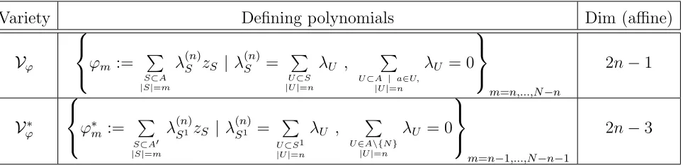
let us summarize all the defining equations in Table 1.

di-Variety Defining polynomials Dim (affine)

Vϕ

 



ϕm := P

S⊂A

|S|=m

λ(_Sn)zS | λ (n)

S =

P

U⊂S

|U|=n

λU ,

P

U⊂A | a∈U,

|U|=n

λU = 0  



m=n,...,N−n

2n−1

V∗ ϕ

 



ϕ∗_m := P

S⊂A0

|S|=m

λ(_Sn1)zS | λ (n) S1 =

P

U⊂S1

|U|=n

λU , P

U∈A\{N} |U|=n

λU = 0  



m=n−1,...,N−n−1

2n−3

Table 1: Summary of defining polynomials for the varieties under consideration. Here, the index set A = {1,2, . . . , N}, A0 ={a ∈ A | a 6= 1, N} and S1 = S∪ {1}. The λ’s are complex coefficients and the varieties are in affine coordinatesz.

mension of the variety by two. For the specific case of n= 2, the (affine) dimension is

1 and therefore we have a 0-dimensional (projective) variety, that is, a set of discrete

points. The degree of each polynomials is {1, . . . , N −3} and from B´ezout’s theorem

(the number of points corresponds to the product of the degree of the polynomials), we

therefore expect for generic choices of the lambda coefficients to have (N −3)! points,

counting multiplicity.

3

Scattering Geometry

We will now study these algebraic varieties in details in order to grasp their geometrical

nature. Noting that for the case n = 2, V∗

ϕ is a discrete set of points corresponding to the solutions of the scattering equation, and noting that this is only one specific case

defined from irreducible representations of the M¨obius group, we will refer to all the

varieties V∗

ϕ and Vϕ asscattering varieties by abuse of terminology.

Indeed, the deep relation of the scattering equations with irreducible representations

of the M¨obius algebra motivates the study of the full class of varieties Vϕ and Vϕ∗.

However, the question of physical significance of the varieties for n 6= 2 still remains

open. Nevertheless, we hope that an understanding of the geometrical structures will

shed light into possible interpretations and the nature of particles scattering. We

3.1

Hilbert series

Let us first find the dimension, degree and Hilbert series of these varieties. We start

by listing all possibles N = 2,3,4,5,6, . . . and tabulate the results. We can extract

these geometrical quantities using standard computational geometric packages, such

as [17,18] as well as software interfacing with Mathematica [19]. The tensor coefficients

from (2.8) are kept as generic non-vanishing parameters λS 6= 0 satisfying the highest

weight condition (2.8).

The Hilbert seriesH(t) is a useful tool to identify the nature of an algebraic variety

V. It has a geometrical interpretation in that it supplies a generating function,

H(t) = ∞ X

i=0

dim_CVi ti , (3.1)

where the quantity dim_CVi is the complex dimension of the graded pieces of V. It thus

represents the number of independent polynomials of degree i on V and this encodes

information about many geometrical features of the variety. Hilbert series also plays a

crucial role in the context of gauge theories [20] to count gauge invariant operators.

For convenience of presentation, we will adopt the standard nomenclature that the

Hilbert series is presented in the second kind, meaning that for an affine variety V, we

have

H(t) = k X

i=0

aiti !

.

(1−t)dimCV , (3.2)

with the power of the denominator being the dimension of the variety and the

numera-tor is a polynomial with integer coefficientsai. (The first kind would have the dimension

of the ambient space as the power of the denominator instead). Furthermore, we will

abbreviate the Hilbert series to simply the sequence of coefficients {a0, a1, . . . , ak}. In this second kind, a useful fact is that the sum overai (i.e., the numerator evaluated

3.1.1 The variety Vϕ

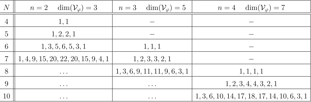
Using this notation, it is expedient to tabulate our findings of the various Hilbert series

obtained through explicit computation [17, 18]. First, before imposing the M¨obius

transformation, we obtain the results for Vϕ presented in Table 2.

N n = 2 dim(Vϕ) = 3 n = 3 dim(Vϕ) = 5 n = 4 dim(Vϕ) = 7

4 1,1 − −

5 1,2,2,1 − −

6 1,3,5,6,5,3,1 1,1,1 −

7 1,4,9,15,20,22,20,15,9,4,1 1,2,3,3,2,1 −

8 . . . 1,3,6,9,11,11,9,6,3,1 1,1,1,1

9 . . . 1,2,3,4,4,3,2,1

10 . . . 1,3,6,10,14,17,18,17,14,10,6,3,1

Table 2: Dimension and Hilbert series for Vϕ. Note that we have recorded the affine dimension here, whereby embedding Vϕ into CN.

A few observations are immediate. First, from combinatorics, all the numerators are

palindromic in thatai =ak−i for all i. This means, by a theorem of Stanley [21, 22], that all the corresponding varieties Vϕ are, in fact, affine Calabi-Yau.§

Next, the sequences of numbers for n = 2 and n = 3 are well-known. The n = 2

case corresponds to the so-calledMahonian triangle, the triangle of Mahonian numbers

Tp,k. One combinatorial definition of these numbers [24] is that it is the number of

permutations π = (π(1), . . . , π(p)) of {1, . . . , p} such that the so-called major index P

π(i)>π(i+1)

i is equal to k. They have a nice generating function which allows us to

§_{Strictly speaking, the module generated by the ideal should be a Cohen-Macaulay graded integral}

analytically write the Hilbert series as a function of N ≥4:

H(t;N)n=2 = (1−t)−3 N−3

Y

j=1 j X

i=0

ti = (1−t)−3X k

TN−3,ktk , (3.3)

This nice analytical formula deduced from our examples allows us to conjecture its

validity for any number of scattering particles N.

Similarly, the n = 3 case corresponds to ak-generalization of lattice permutations.

As a function of N ≥7 (the initial case of N = 6 has the numerator 1 +t+t2 _which does not obey the following generating function), we have:

H(t;N)n=3 = (1−t)−5 N−4

Y

j=1

Cj+1(t) ; Cj(t) :=

Y

0<k<j, gcd(k,j)=1

(t−e2πikj_{) , (3.4)}

where, in the above, Cj(t) are the cyclotomic polynomials. Again, a nice analytical formula supports the conjecture for its validity up to any N value.¶

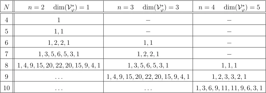
3.1.2 The variety V∗ ϕ

After fixing variables of the above varieties by two M¨obius transformations, z1 → ∞ and zN → 0, the complex (affine) dimension of the variety uniformly drops by 2 and

we obtain the algebraic varieties V∗

ϕ. Again, Hilbert series can be obtained through explicit computation [17, 18] and the resulting Hilbert series are summarized in Table

3.

We observe that these Hilbert series are simply a shift of the above table. For the

case n = 2, we recover the same Hilbert series as for the Vϕ case, shifted from N to

N + 1. For the other cases, the Hilbert series for n correspond to that of Vϕ forn−1

shifted fromN toN+ 2. This is reminiscent from the fact that the number of variables

decreases by 2 when M¨obius invariance is fixed. Thus, we find again the Mahonian

numbers, however now for both the n = 2 and n = 3 cases, and the cyclotomic

polynomials for the n= 4 case.

¶_{It would be interesting to find similar constructions for the following cases withn≥4, which is}

N n = 2 dim(V∗

ϕ) = 1 n= 3 dim(Vϕ∗) = 3 n = 4 dim(Vϕ∗) = 5

4 1 − −

5 1,1 − −

6 1,2,2,1 1,1 −

7 1,3,5,6,5,3,1 1,2,2,1 −

8 1,4,9,15,20,22,20,15,9,4,1 1,3,5,6,5,3,1 1,1,1

9 . . . 1,4,9,15,20,22,20,15,9,4,1 1,2,3,3,2,1

10 . . . 1,3,6,9,11,11,9,6,3,1

Table 3: Affine dimension and Hilbert series forV∗ ϕ.

This observation unveils deep connections across the varietiesVϕandVϕ∗for different

particle numbers N. We should note, however, that Hilbert series are not topological

invariants as it can be presented in many ways. In fact, they depend on the embedding

of the variety within the polynomial ring. This means that we cannot conclude that

we have identical varieties when they share the same Hilbert series. Nevertheless, the

Calabi–Yau property is deducible from the palindromic nature and it is remarkable

that that the scattering varieties are all affine Calabi–Yau manifolds without recourse

to supersymmetry or string theory.

3.2

Resolution and Betti numbers

Having established the correspondence between the dimension of the graded pieces of

Vϕ andVϕ∗ via the Hilbert series, let us see whether we can highlight further similarities or differences. For instance, one could examine the resolution of the module M =

R/V where R the polynomial ring _C[z1, . . . , zN] for Vϕ and C[z2, . . . , zN−1] for Vϕ∗ and V is the corresponding variety ideal. Remarkably, it turns out that the Betti

numbers corresponding to this resolution follow a predictable pattern as we now see.

We emphasize that the Betti number here are not the usual topological Betti numbers

of which one is more familiar. The Betti numbers henceforth refers to the notation

idealk.

Let us start by exemplifying the resolution of the module corresponding to the

somewhat trivial case of V∗

ϕ for n = 2, e.g. the discrete set of points. Considering

N = 4, we have the following ideal:

V₄∗ =hλ12z2+λ13z3i , (3.5)

with the tensor coefficientsλ12 and λ13 subject to the highest weight condition (2.16). In this case, this translates to λ12 +λ13+λ23 = 0, and, since λ23 does not appear in the ideal, the parameters λ12 and λ13 can be considered as generic parameters (provided that λ23 takes the adequate value). The minimal resolution of the module

M₄∗ =_C[z2, z3]/V4∗ gives to the short exact sequence

0←−M₄∗ ←− R1 ←−−−−−−−−−

z2+(λ13/λ12)z3

R1 ←− 0 (3.6)

with the Betti numbers

i\j 0 1

0 1 1

Total 1 1

This tally means that thej-th column of thei-th row gives the number of basis elements

of degreei+j in the free moduleM₄∗[j] of shifted degreej (e.g., in this case,M₄∗[0] =R1 and M₄∗[1] = R1_{). The total corresponds to the Betti numbers, giving the number of} copies of the polynomial ringR=_C[z2, z3], meaningRi =⊕iRwithithe corresponding Betti number.

Using [17, 18], we easily obtain the tally for the Betti numbers of resolutions of

other modulesM_N∗. For instance, still consideringn = 2, we find forN = 5 andN = 6,

respectively:

k_{More information on the meaning of Betti numbers of minimal resolution of zero-dimensional}

N = 5 N = 6

i\j 0 1 2

0 1 1 0

1 0 1 1

Total 1 2 1

i\j 0 1 2 3

0 1 1 0 0

1 0 1 1 0

2 0 1 1 0

3 0 0 1 1

Total 1 3 3 1

What about theV varieties? For comparison, let us present the tally corresponding

to the Betti numbers of the resolution of the module defining the varietiesVϕ forn= 2

and N = 4, N = 5 andN = 6. We obtain:

N = 4 N = 5 N = 6

i\j 0 1

0 1 0

1 0 1

Total 1 1

i\j 0 1 2

0 1 0 0

1 0 1 0

2 0 1 0

3 0 0 1

Total 1 2 1

i\j 0 1 2 3

0 1 0 0 0

1 0 1 0 0

2 0 1 0 0

3 0 1 1 0

4 0 0 1 0

5 0 0 1 0

6 0 0 0 1

Total 1 3 3 1

Interestingly, we notice that the total matches the one for the varieties where M¨obius

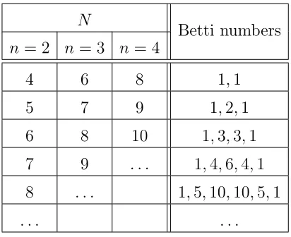
We summarise the Betti numbers in Table 4. Both the varieties Vϕ and Vϕ∗ share the

same Betti numbers for the resolution of their module, when they have equal number of

particles N. Moreover, the sequence is repeated for variousn, with a shiftN →N+ 2

when n→n+ 1.

N

Betti numbers

n= 2 n = 3 n= 4

4 6 8 1,1

5 7 9 1,2,1

6 8 10 1,3,3,1

7 9 . . . 1,4,6,4,1

8 . . . 1,5,10,10,5,1

. . . .

Table 4: Betti numbers of the module free resolution for the varieties Vϕ and Vϕ∗, with respect to the number of particlesN and the highest weight degree n.

We clearly see a pattern and we can conjecture that it holds for every remaining

varieties. The minimal resolution of the modulesM and M∗ will be an exact sequence

with the numbers of generators forming Pascal’s triangle; a generating function for the

Betti numbers is then obtained from (1 +x)N−2n+1.

With these Betti numbers, we can also note that the length of the resolution is

equal to N − 3. Thus, we always have the codimension of M (and M∗) equal to

the length of its resolution, thus all the quotient rings considered are arithmetically

Cohen–Macaulay.

3.3

Calabi–Yau geometry

Are the varieties of geometrical significance, or, at least, of some familiarity? Let us

focus on the cases of affine dimension 3. These are the cases with n = 2 and n = 3,

respectively before and after M¨obius fixing, with a shift of two in N.

numerator and the denominator is factorized as a product of (1−ti) for some i

coef-ficients. We obtain H(t) = (1−t)−4(1−t2) and can readily identify [20] the Hilbert series of the famous conifold as as an affine (non-compact) CY3 , given by a quadric in_C4_.

The next variety has H(t) = (1−t)−3(1 + 2t+ 2t+t2) which is, when put into the Euler form, H(t) = (1−t2)(1−t3)/(1−t)5. This means we have the intersection of a quadric and a cubic in _C5. Upon projectivizing to _CP4, this is a complete intersection which gives a K3 surface of degree 6 and (geometric) genus 4 [26].

Continuing in a similar fashion, we can identify all the dimension 3 (projective

dimension 2) cases as complete intersection complex surfaces and use the standard

notation [27]:

[n|k1, k2, . . . , km] := {intersection of m degree ki hypersurfaces in CPn} . (3.7)

With this notation, the K3 condition, that is vanishing of the first Chern class, is

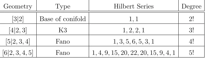
equivalent to Pm_i=1ki =n+ 1. Similarly, a condition for being a Fano variety, is that the left-hand side of this expression is greater, that is Pm_i=1ki > n+ 1. We can thus summarize the (projective) geometries as in Table 5.

Geometry Type Hilbert Series Degree

[3|2] Base of conifold 1,1 2!

[4|2,3] K3 1,2,2,1 3!

[5|2,3,4] Fano 1,3,5,6,5,3,1 4!

[6|2,3,4,5] Fano 1,4,9,15,20,22,20,15,9,4,1 5!

Table 5: Geometry of the affine3-dimensional (and hence, projective dimension 2) varieties. TheType refers to the base B after projectivisation of the varieties.

The regularity of this table easily allows to speculate on the nature of the

follow-ing geometries for greater N. We expect thus all remaining 3-dimensional algebraic

varieties to be Fano, as presented in Table 6.

Moreover, we should emphasize that, by the palindromic nature of the Hilbert

Geometry Type Hilbert Series Degree

Vϕ [N −1|2,3,4, . . . , N −2] Fano {TN−3,k}_∀k (N −2)!

V∗

ϕ [N −3|2,3,4, . . . , N −4] Fano {TN−5,k}_∀k (N −4)!

Table 6: General description of the affine 3-dimensional geometry for Vϕ with N ≥6 and

V∗

ϕ with N ≥8.

(unprojectivized) 3-dimensional varieties. They can therefore be considered as complex

cones over some compact base surface, precisely in the same way as in the Calabi-Yau

singularities of AdS5/CF T4.

3.4

Singular locus

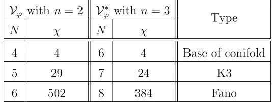
One might wonder then, what is the difference between the varieties Vϕ and Vϕ∗ from

a geometrical standpoint? Calculating the Euler number χ of the above projective

varieties unveils more information about the nature of the geometry considered. In

this section, we concentrate our study on the cases of 3-dimensional varieties, that is

Vϕ for n= 2 and Vϕ∗ forn = 3. Our findings forχ using [17, 18] are presented in Table 7.

Vϕ with n = 2 Vϕ∗ with n = 3 _Type

N χ N χ

4 4 6 4 Base of conifold

5 29 7 24 K3

6 502 8 384 Fano

Table 7: Euler numbers χ for the 3-dimensional varieties encountered.

We find,

hp,q(B4,2) =

h0,0

h0,1 h0,1

h0,2 _h1,1 _h0,2

h0,1 _h0,1

h0,0

=

1

0 0

0 2 0

0 0

1

, (3.8)

where we use the notation BN,n for the projective variety corresponding to Vϕ with N

particles and highest weight polynomial of degreen. This Hodge diamond corresponds

to the one of the conifold, as expected. Furthermore, we find that

hp,q(B∗_6,3) =hp,q(B4,2) (3.9)

for the corresponding variety B∗ _{resulting from fixing M¨obius invariance. The Hodge}

diamonds for the other varieties present in Table 7 are, for the K3 surfaces:

hp,q(B5,2) =

1

0 0

1 25 1

0 0

1

, hp,q(B₇∗_,3) =

1

0 0

1 20 1

0 0

1

, (3.10)

and for the Fano varieties:

hp,q(B6,2) =

1

0 0

49 402 49

0 0

1

, hp,q(B₈∗_,3) =

1

0 0

49 284 49

0 0

1

. (3.11)

corresponding to the K3 surface and be puzzled. Here, we have a K3 surface as a

complete intersection of a quadric and a cubic in _CP4. Should the Euler number then not be the standard 24? Upon inspection of the defining polynomials from (2.10), we

see that the tensor coefficientsλto these polynomials inz are not generic and obey the

physical constraints (2.8). In other words, we are not in a generic point in the complex

structure moduli space of K3 surfaces but quite special ones. In fact, we will now see

that the scattering varietiesVϕ forn = 2 all contain singularities and are therefore not

smooth, which will deviate the values of the Euler number from generic varieties.

The singular locus of an algebraic variety corresponds to its intersection with the

Jacobian ideal, i.e., the zero locus of its Jacobian matrix, giving the variety, for that

defined by (2.10),

J =



    

∂ϕn

∂z1 . . .

∂ϕn

∂zN

..

. . . . ...

∂ϕN−n

∂z1 . . .

∂ϕN−n

∂zN



    

= 0 . (3.12)

Let us write indicesi= 1, . . . , N forz and m=n, . . . , N−n forϕ. Therefore, we have

∂ϕm

∂zi

= X

S⊂A | i∈S,

|S|=m

λ(_Sn)zS\{i} . (3.13)

We should realise that each polynomial from the Jacobian corresponds to the limit

where the variable zi → ∞ as this is the effect of the action from the operators

Lzi =

∂

∂zi, as can be seen by generalisation of the z1 variable case (2.14). From the

ideal generated by these partial derivatives — the Jacobian ideal — we therefore have

N−2n+ 1 polynomials of degree ranging fromn−1 toN−n−1, for eachi= 1, . . . , N,

defining an algebraic variety in_CPN−1.

Let us focus on the important case of n = 2. First, for N = 4, we have only one

homogeneous degree 2 polynomial{˜h2}. Explicitly,

The corresponding Jacobian ideal is then

J4 =hλ12z2+λ13z3 +λ14z4, λ12z1+λ23z3+λ24z4,

λ13z1+λ23z2 +λ34z4, λ14z1+λ24z2+λ34z3i . (3.15)

We readily see that for arbitrary generic choices of λ, the only point in J4 is when all zi = 0, which in C4 is the origin and in CP3 is excluded. Hence, for this generic case, the quadric projective variety [3|2] is smooth and as an affine variety is realized

as the conifold, with the familiar singularity at the origin corresponding to the tip of

the cone.

However, for irreducible representation of the M¨obius group, the tensor coefficients

λ are not generic. They must satisfy the constraints of highest weight (2.8), that is,

      

     

λ12+λ13+λ14 = 0,

λ12+λ23+λ24 = 0,

λ13+λ23+λ34 = 0,

λ14+λ24+λ34 = 0.

(3.16)

In this case, we can find a one-parameter family of solutions toV4 andJ4 given by the following,

(z1, z2, z3, z4) = (x, x, x, x) , x∈C . (3.17) This gives the singular locus on our non-generic variety. On the affine variety, the singular locus is a ray from the origin while, on the projective variety, it is a single

Next, for the N = 5 case, we have a quadric intersecting a cubic. Explicitly,

V5 = h λ12z1z2+λ13z1z3+λ14z1z4+λ15z1z5+λ23z2z3

+λ24z2z4+λ25z2z5+λ34z3z4+λ35z3z5+λ45z4z5 ,

(λ12+λ13+λ23)z1z2z3+ (λ12+λ14+λ24)z1z2z4

+(λ12+λ15+λ25)z1z2z5+ (λ13+λ14+λ34)z1z3z4

+(λ13+λ15+λ35)z1z3z5+ (λ14+λ15+λ45)z1z4z5

+(λ23+λ24+λ34)z2z3z4+ (λ23+λ25+λ35)z2z3z5

+(λ24+λ25+λ45)z2z4z5+ (λ34+λ35+λ45)z3z4z5 i , (3.18)

where the highest weight (2.8) constraints on the coefficients are:

         

        

λ12+λ13+λ14+λ15= 0 ,

λ12+λ23+λ24+λ25= 0 ,

λ13+λ23+λ34+λ35= 0 ,

λ14+λ24+λ34+λ45= 0 ,

λ15+λ25+λ35+λ45= 0 .

(3.19)

This gives a non-generic K3 surface upon projectivization. The corresponding Jacobian

J5 = h λ12z2+λ13z3 +λ14z4+λ15z5, λ12z1+λ23z3+λ24z4+λ25z5,

λ13z1+λ23z2+λ34z4+λ35z5, λ14z1+λ24z2+λ34z3+λ45z5,

λ15z1+λ25z2+λ35z3+λ45z4, (λ12+λ13+λ23)z2z3

+(λ12+λ14+λ24)z2z4+ (λ12+λ15+λ25)z2z5+ (λ13+λ14+λ34)z3z4

+(λ13+λ15+λ35)z3z5+ (λ14+λ15+λ45)z4z5, (λ12+λ13+λ23)z1z3

+(λ12+λ14+λ24)z1z4+ (λ12+λ15+λ25)z1z5+ (λ23+λ24+λ34)z3z4

+(λ23+λ25+λ35)z3z5+ (λ24+λ25+λ45)z4z5, (λ12+λ13+λ23)z1z2

+(λ13+λ14+λ34)z1z4+ (λ13+λ15+λ35)z1z5+ (λ23+λ24+λ34)z2z4

+(λ23+λ25+λ35)z2z5+ (λ34+λ35+λ45)z4z5, (λ12+λ14+λ24)z1z2

+(λ13+λ14+λ34)z1z3+ (λ14+λ15+λ45)z1z5+ (λ23+λ24+λ34)z2z3

+(λ24+λ25+λ45)z2z5+ (λ34+λ35+λ45)z3z5, (λ12+λ15+λ25)z1z2

+(λ13+λ15+λ35)z1z3+ (λ14+λ15+λ45)z1z4+ (λ23+λ25+λ35)z2z3

+(λ24+λ25+λ45)z2z4+ (λ34+λ35+λ45)z3z4 i . (3.20)

Again, looking at the terms inJ5 linear in z, we see that on the ray from the origin,

(z1, z2, z3, z4, z5) = (x, x, x, x, x), x∈C, (3.21)

the solution set of the highest weight conditions (3.19) is exactly what is required to

make the five linear polynomials in (3.20) vanish. In fact, one can see that for all N,

the set of linear constraints on the coefficientsλ will exactly make the Jacobian vanish

for the ray (x, x, . . . , x) whereby making the projective point [1 : 1 : . . . : 1] always a

singular point on the scattering varieties Vϕ forn = 2.

To demonstrate this, let us write the highest weight (2.8) condition for n = 2 as

follows:

 

 X

i∈A\{r}

λri = 0  

 ∀r∈A

(3.22)

This constitutes of a set ofN equations for eachrinA. Now, for one specific constraint

with index r0, each term λr0_i with i∈ A\{r0} will appear once (and only once) in the

corresponding i index. This means that summing all equations for which r 6= r0 and

removing the one with r = r0 leads to a constraint involving only the terms λij for

which i, j ∈ A\{r0_{}. (Each of those terms will appear twice from symmetry of the}

indices.) This gives another set of identities:

 



X

i,j∈A\{r}, i<j

λij = 0  

 ∀r∈A

(3.23)

As an illustration, we can take the caseN = 5 for which the highest weight conditions

are explicitly given in (3.19). Let us choose the index r0 = 1. Adding the last four

equations from (3.19) minus the first one leads to 2(λ23+λ24+λ25+λ34+λ35+λ45) = 0 and we see that the sum of all λ terms with indices in A\{1} must vanish, as stated

in (3.23). The remaining equations in (3.23) follows from the different choices ofr0.

We should also recast the Jacobian ideal in the following form (altogetherN(N−3)

polynomials):

P

p∈A\{r}

( P

i<j|{i,j}⊂{p,r}

λij)zp = 0, ∀r∈A ,

P

p,q∈A\{r}

( P

i<j|{i,j}⊂{p,q,r}

λij)zpzq= 0, ∀r ∈A ,

P

p,q,u∈A\{r}

( P

i<j|{i,j}⊂{p,q,u,r}

λij)zpzqzu = 0, ∀r ∈A ,

.. .

P

p1,...,pN−3∈A\{r}

( P

i<j|{i,j}⊂{p1,...,pN−3,r}

λij)zp1...zpN−3 = 0, ∀r ∈A .

(3.24)

Our claim is that, after taking all the z variables to be x ∈ _C, each condition in (3.24) are automatically satisfied. Indeed, in this case, we can factor out all the x

variables and the firstN equations with degree 1 simply vanish by virtue of the highest

weight conditions (2.8). For the remaining equations of degree d > 1, the conditions

can be rewritten as follows after some combinatorial reorganisation:





N −2

d−1

X

i∈A\{r}

λir+

N −3

d−2

X

p,q∈A\{r}, p<q

λpq 

We can see that the coefficients involving theλterms vanish since we have P i∈A\{r}

λir = 0

from (3.22) and P p,q∈A\{r}, p<q

λpq = 0 from (3.23). Therefore all the equations (3.24) are

satisfied for the point (x, x, . . . , x), making the projective point [1 : 1 : . . . : 1] always

singular.

It is remarkable that the existence of this singularity is deeply rooted into the

constraint from highest weight (2.8), and hence the fact that the polynomial system

form an irreducible representation of the M¨obius algebra.

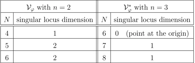
This singularity is however not the only one. A full geometrical description is

somewhat involved and we simply content ourselves with observing the dimension, as

summarised in Table 8.

Vϕ with n = 2 Vϕ∗ with n= 3

N singular locus dimension N singular locus dimension

4 1 6 0 (point at the origin)

5 2 7 1

6 2 8 1

Table 8: Affine dimension of the singular locus of the corresponding3-dimensional varieties.

We see that the constraints (2.16) on the tensor coefficients λ for V∗_{, reminiscent}

from the highest weight conditions, also implies the existence of singularities. However,

the nature of such singularities is different from the corresponding 3-dimensional

va-rieties Vϕ as they differ in their dimension and produce different topological numbers,

such as the Euler characteristicχ and the Hodge diamond.

4

Discussion and Outlook

In this work, we presented geometrical properties of algebraic varieties built up from

irreducible representations of the M¨obius algebra in the hope that it will help to shed

light on their physical meaning and, as a consequence, on the understanding of the

We found that these varieties are allaffine Calabi-Yau manifolds with Hilbert series following very regular pattern, such as the Mahonian triangles or the cyclotomic

poly-nomials. For the physical M¨obius invariant three-dimensional varieties, we furthermore

found that they consist of familiar geometries such as theconifold for the scattering of four particles, a cone over aK3 surface for five particles and a cone overFanosurfaces (i.e., del Pezzo surfaces) for six and seven particles.

In addition, computation of the Euler number and Hodge diamonds showed that

not only are the affine Calabi-Yau spaces singular, but so too are their projectivizations

to compact surfaces. A short computation unveiled that the singular points are related

to the conditions for the polynomial system to be an irreducible representation of the

M¨obius algebra. The singularity contains at least one point for the projective varieties

and it would be expedient to understand its physical meaning. Indeed, the physical

constraints on the momenta and hence coefficients in the scattering variety show that

we are in very special singular points in the complex structure moduli space.

It would be interesting to develop further the geometrical properties, such as Hodge

numbers for more varieties, and a complete description of the singularity geometry.

Furthermore, our study focused on generic parameters and very special momenta

con-figurations might lead to extra geometrical structures. It would be interesting to

inves-tigate the way the varieties degenerate when one (or more) of the polynomial coefficient

λS vanishes and understand the dependence of the geometrical properties of the

va-rieties on the structure of these coefficients. Understanding the physical meaning of

the above varieties is of crucial importance and we hope that our analyses for the

geo-metrical structure of the scattering variety offer a good starting point to unveil deeper

connections.

Acknowledgements

YHH would like to thank the Science and Technology Facilities Council, UK, for an

Advanced Fellowship and for STFC grant ST/J00037X/1, the Chinese Ministry of

Education, for a Chang-Jiang Chair Professorship at NanKai University, the city of

Tian-Jin for a Qian-Ren Scholarship, the US NSF for grant CCF-1048082, as well as

Oxford, for their enduring support. CM is grateful to Hwasung Lee for helpful

discus-sions as well as City University, London and Helios Technology for giving the possibility

to pursue this work.

References

[1] F. Cachazo, S. He and E. Y. Yuan, “Scattering in Three Dimensions from Rational

Maps,” JHEP 1310 (2013) 141 [arXiv:1306.2962 [hep-th]].

[2] F. Cachazo, S. He and E. Y. Yuan, “Scattering Equations and KLT

Orthogonal-ity,” arXiv:1306.6575 [hep-th].

[3] F. Cachazo, S. He and E. Y. Yuan, “Scattering of Massless Particles in Arbitrary

Dimension,” arXiv:1307.2199 [hep-th].

[4] F. Cachazo, S. He and E. Y. Yuan, “Scattering of Massless Particles: Scalars,

Gluons and Gravitons,” arXiv:1309.0885 [hep-th].

[5] L. Dolan and P. Goddard, “Proof of the Formula of Cachazo, He and Yuan for

Yang-Mills Tree Amplitudes in Arbitrary Dimension,” arXiv:1311.5200 [hep-th].

[6] L. Dolan and P. Goddard, “The Polynomial Form of the Scattering Equations,”

arXiv:1402.7374 [hep-th].

[7] S. Weinzierl, “On the solutions of the scattering equations,” arXiv:1402.2516

[hep-th].

[8] S. G. Naculich, “Scattering equations and BCJ relations for gauge and

gravita-tional amplitudes with massive scalar particles,” arXiv:1407.7836 [hep-th].

[9] S. G. Naculich, “Scattering equations and virtuous kinematic numerators and

dual-trace functions,” JHEP 1407 (2014) 143 [arXiv:1404.7141 [hep-th]].

[10] F. Cachazo and D. Skinner,Gravity from Rational Curves, ArXiv e-prints(2012) [http://xxx.lanl.gov/abs/1207.0741arXiv:1207.0741].

[11] Y.-t. Huang and S. Lee, A New Integral Formula for Supersymmetric Scattering

Amplitudes in Three Dimensions, Physical Review Letters 109 (2012) 191601,

[12] E. Witten,Perturbative Gauge Theory as a String Theory in Twistor Space,

Com-munications in Mathematical Physics 252 (2004) 189–258, [http://xxx.lanl.

gov/abs/hep-th/0312171hep-th/0312171].

[13] R. Roiban, M. Spradlin, and A. Volovich,Tree-Level S-Matrix of Yang-Mills

The-ory, Physical Review D 70 (2004) 026009, [http://xxx.lanl.gov/abs/hep-th/

0403190hep-th/0403190].

[14] F. Cachazo and Y. Geyer, A “Twistor String” Inspired Formula For Tree-Level

Scattering Amplitudes in N = 8 SUGRA, ArXiv e-prints (2012) [http://xxx.

lanl.gov/abs/1206.6511arXiv:1206.6511].

[15] M. Spradlin and A. Volovich, “From Twistor String Theory To Recursion

Rela-tions,” Phys. Rev. D 80, 085022 (2009) [arXiv:0909.0229 [hep-th]].

[16] S. T. Alsid and M. A. Serna, “Unifying Geometrical Representations of Gauge

Theory,” arXiv:1308.1092 [hep-th].

[17] Decker, W.; Greuel, G.-M.; Pfister, G.; Sch¨onemann, H.: Singular 3-1-6 — A

computer algebra system for polynomial computations.

http://www.singular.uni-kl.de (2012).

[18] D. Grayson and M. Stillman, “Macaulay 2, a software system for research in

algebraic geometry.” Available athttp://www.math.uiuc.edu/Macaulay2/.

[19] J. Gray, Y. -H. He, A. Ilderton and A. Lukas, “STRINGVACUA: A Mathematica

Package for Studying Vacuum Configurations in String Phenomenology,” Comput.

Phys. Commun. 180, 107 (2009) [arXiv:0801.1508 [hep-th]].

[20] S. Benvenuti, B. Feng, A. Hanany and Y. -H. He, “Counting BPS Operators

in Gauge Theories: Quivers, Syzygies and Plethystics,” JHEP 0711, 050 (2007) [hep-th/0608050].

[21] R. Stanley, “Hilbert functions of graded algebras,” Adv. Math. 28 (1978), 57-83.

[22] D. Forcella, A. Hanany, Y. -H. He and A. Zaffaroni, “The Master Space of N=1

Gauge Theories,” JHEP 0808, 012 (2008) [arXiv:0801.1585 [hep-th]].

[23] Y. H. He, V. Jejjala, C. Matti, B. D. Nelson and M. Stillman, “The Geometry of

[24] N. Sloane et al.,”The On-Line Encyclopedia of Integer Sequences”, https://

oeis.org/

[25] Anna Lorenzini, “Betti numbers of points in projective space”, Journal of Pure

and Applied Algebra, Volume 63, Issue 2, 12 March 1990, Pages 181193

[26] G Brown, “A database of polarized K3 surfaces”, Experiment. Math. 16 (1), 2007,

7-20.

[27] T. Hubsch, “Calabi-Yau Manifolds: a Bestiary for Physicists,” World Scientific,