The hydrological flux of organic carbon at the catchment scale: a case study in the Cotter River catchment, Australia

Full text

(1)The Hydrological Flux of Organic Carbon at the Catchment Scale: a Case Study in the Cotter River Catchment, Australia. Karim Sabetraftar. December 2005. A thesis submitted for the degree of Doctor of Philosophy of. The Australian National University.

(2) Statement of Originality. This thesis is my own work and it contains no material which has previously been accepted for the award of any other degree in any other university. The thesis contains no material written by any other person, except where due reference is made in the text.. Karim Sabetraftar. December 2005. ii.

(3) Acknowledgments I am sincerely grateful for the contribution provided by all members of my supervisory panel. The panel included Professor Brendan Mackey (Chair), Dr Barry Croke and Dr Stephen Roxburgh. I am especially grateful to Barry Croke who provided many valued technical suggestions. I also acknowledge the excellent guidance, motivation and advice provided by Professor Brendan Mackey and Dr Stephen Roxburgh.. I was fortunate to receive contributions and assistance from the other advisers who were especially helpful in the project. They were Dr John Banks, Professor Anthony Jakeman, Dr Lachlan Newham, Dr Michael Roderick, Dr Sandy Berry, Dr John Gallant, Dr A Malcolm Gill, Dr Janette Lindesay and Dr Robyn Harris. Dan Diaconu, Bronwyn Trevethan, Clem Davis and Sue Nichols also assisted greatly with preparation of the hydrologic and climate data sets. Dr Mike Hutchinson provided the high resolution DEM used in this case study.. The Ministry of Science & Research and Technology, Giulan University in Iran and the Cooperative Research Centre (CRC) for Greenhouse Accounting at the Australian National University supported this research. I am also most appreciative of the support from Environment ACT especially from Trish Macdonald, ECOWISE Environment particularly Tanya Whiteway and Sarah Sharp, ACTEW Corporation, CSIRO Forestry in particular Dr John Raison and Dr Heather Keith, CSIRO Land & Water especially Professor Rob Vertessy, Dr Sue Vink, Dr Neil McKenzie and Dr Hamish Cresswell and University of Canberra (UC) particularly Dr Fiona Dyer. Water quality data was analysed by John Pengelly at the MurrayDarling Freshwater Research Centre (MDFRC), CSIRO Land & Water, Albury, NSW.. I would like to thank the staff of the School of Resources, Environment & Society (SRES) for their support over the course of the project. Particularly, I would like to thank Dr Susanne Holzknecht for editing advice on my thesis, Steve Leahy and Karl Nissen for IT support, Clive Hilliker for Cartography and Design work, Jane Bryan and Jean Rivard who assisted by providing much valued GIS guidance, Mark Lewis for assistance with finances, Piers Bairstow and Mauro Davanzo for field services and in particular Professor Peter Kanowski and Dr Richard Greene for their valuable support during my research and thesis preparation.. Finally, I would like to acknowledge the great support of Fatemeh and my girls Shamim and Sheida and I would also like to acknowledge the previous boundless support of my Dad and Mum.. iii.

(4) Abstract Existing terrestrial carbon accounting models have mainly investigated atmosphere-vegetationsoil stocks and fluxes but have largely ignored the hydrological flux of organic carbon. It is generally assumed that biomass and soil carbon are the only relevant pools in a landscape ecosystem. However, recent findings have suggested that significant amounts of organic carbon can dissolve (dissolved organic carbon or DOC) or particulate (particulate organic carbon or POC) in water and enter the hydrological flux at the catchment scale. A significant quantity of total organic carbon (TOC) sequestered through photosynthesis may be exported from the landscape through the hydrological flux and stored in downstream stocks.. This thesis presents a catchment-scale case study investigation into the export of organic carbon through a river system in comparison with carbon that is produced by vegetation through photosynthesis. The Cotter River Catchment was selected as the case study. It is a forested catchment that experienced a major wildfire event in January 2003. The approach is based on an integration of a number of models. The main input data were time series of in-stream carbon measurements and remotely sensed vegetation greenness. The application of models to investigate diffuse chemical substances has dramatically increased in the past few years because of the significant role of hydrology in controlling ecosystem exchange. The research firstly discusses the use of a hydrological simulation model (IHACRES) to analyse organic carbon samples from stream and tributaries in the Cotter River Catchment case study. The IHACRES rainfall-runoff model and a regionalization method are used to estimate stream-flow for the 75 sub-catchments. The simulated streamflow data were used to calculate organic carbon loads from concentrations sampled at five locations in the catchment.. The gross primary productivity (GPP) of the vegetation cover in the catchment was estimated using a radiation use efficiency (RUE) model driven by MODIS TERRA data on vegetation greenness and modeled surface irradiance (RS). The relationship between total organic carbon discharged in-stream and total carbon uptake by plants was assessed using a cross-correlation analysis.. The IHACRES rainfall-runoff model was successfully calibrated at three gauged sites and performed well. The results of the calibration procedure were used in the regionalization method that enabled streamflow to be estimated at ungauged locations including the seven sampling sites and the 75 sub-catchment areas. The IHACRES modelling approach was found appropriate for investigating a wide range of issues related to the hydrological export of organic carbon at. iv.

(5) the catchment scale. A weekly sampling program was implemented to provide estimates of TOC, DOC and POC concentrations in the Cotter River Catchment between July 2003 and June 2004. The organic carbon load was estimated using an averaging method.. The rate of photosynthesis by vegetation (GPP) was successfully estimated using the radiation use efficiency model to discern general patterns of vegetation productivity at sub-catchment scales. This analysis required detailed spatial resolution of the GPP across the entire catchment area (comprising 75 sub-catchment areas) in addition to the sampling locations. Important factors that varied at the catchment scale during the sampling period July 2003 – June 2004, particularly the wildfire impacts, were also considered in this assessment.. The results of the hydrologic modelling approach and terrestrial GPP outcome were compared using cross correlation and regression analysis. This comparison revealed the likely proportion of catchment GPP that contributes to in-stream hydrological flux of organic carbon. TOC Load was 0.45% of GPP and 22.5 - 25% of litter layer. As a result of this investigation and giving due consideration to the uncertainties in the approach, it can be concluded that the hydrological flux of organic carbon in a forested catchment is a function of gross primary productivity.. v.

(6) Table of Contents Statement of Originality…………………………………………………………………….ii Acknowledgments………………………………………………………………………….iii Abstract……………………………………………………………………………………..iv Table of Contents…………………………………………………………………………...vi List of Figures……………………………………………………………………………....xi List of Tables……………………………………………………………………………….xv List of Appendices………………………………………………………………………….xviii. Chapter One: Introduction……………………………………………………………….1 1.1 Global carbon and water cycle………………………………………………………….1 1.2 Significance of organic carbon in streams and rivers…………………………………..6 1.3 Research questions and objectives……………………………………………………...9 1.4 Outline of the thesis…………………………………………………………………….12. Chapter Two: Methodological Overview………………………………………………..14 2.1 Introduction…………………………………………………………………………….14 2.2 The link between hydrological flow and organic carbon fluxes……………………….14 2.3 Quantitative predictive framework for hydrological flux of organic carbon ………….15 2.4 Organic carbon pathways in streams…………………………………………………...17 2.5 Models of river ecosystems…………………………………………………………….19 2.5.1 River Continuum Concept………………………………………………………….20 2.5.2 Flood Pulse Concept………………………………………………………………..21 2.5.3 A Hybrid or Coupled Concept……………………………………………………...22 2.6 Chapter summary…………………………………………………………………….....26 Chapter Three: The Cotter River Catchment case study………………………………27 3.1 Study area………………………………………………………………………………27 3.1.1 General description…………………………………………………………………27 vi.

(7) 3.1.2 Location……………………………………………………………………………..27 3.1.3 Climate, Hydrology and Topography..……………………………………………...31 3.1.3.1 Environmental time series data………………………………………………....32 3.1.4 Vegetation and land cover…………………………………………………………..41 3.1.5 Regional Geology and Soils………………………………………………………...45 3.1.6 Land use…………………………………………………………………………….49 3.2 Wildfire impacts on study area………………………………………………………....50 3.2.1 Fire History…………………………………………………………………………50 3.2.2 Wildfire impacts on Vegetation………………………………………………….....55 3.2.3 Wildfires impacts on Streamflow and Aquatic Ecosystems………………………..57 3.2.4: Wildfire impacts on Soils…………………………………………………………..59 3.4 Chapter summary……………………………………………………………………….69. Chapter Four: Hydrologic Modelling……………………………………………………70 4.1 Introduction…………………………………………………………………………….70 4.2 IHACRES selection…………………………………………………………………….73 4.3 IHACRES model description…………………………………………………………...73 4.3.1 Non-Linear module…………………………………………………………………75 4.3.2 Unit hydrograph and linear module………………………………………………...76 4.4 Data preparation………………………………………………………………………...78 4.4.1 Rainfall……………………………………………………………………………...79 4.4.2 Temperature………………………………………………………………………...80 4.5 Data processing…………………………………………………………………………81 4.5.1 Hydrological analysis……………………………………………………………....81 4.5.2 Spatial analysis……………………………………………………………………..82 4.5.2.1 DEM processing………………………………………………………………..82 4.5.2.2 DEM aggregation………………………………………………………………82 4.5.2.3 Depression layers……………………………………………………………….83. vii.

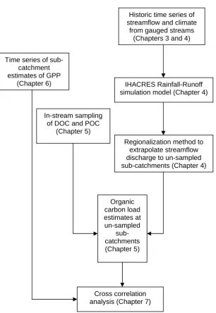
(8) 4.5.2.4 Slope and flow direction………………………………………………………..83 4.5.2.5 Catchment recognition and streamflow network……………………………….83 4.6 Hydrologic model development and estimation of parameters at gauged locations……89 4.6.1 Model calibration…………………………………………………………………...89 4.6.2 Calibration outcomes……………………………………………………………….91 4.6.3 Simulation…………………………………………………………………………..97 4.6.4 IHACRES rainfall-runoff model discussion………………………………………..102 4.7 Regionalization method and parameters estimation at ungauged locations…………....103 4.7.1 General description…………………………………………………………………103 4.7.2 Regionalization of IHACRES………………………………………………………110 4.7.3 Catchment response characteristics………………………………………………...111 4.7.3.1 Mean annual runoff coefficient………………………………………………....111 4.7.3.2 Flow duration curves and base flow filter……………………………………....117 4.7.3.3 Unit hydrograph………………………………………………………………...117 4.7.4 Regionalization results and model parameters at ungauged locations……………...120 4.8 Chapter summary……………………………………………………………………….126. Chapter Five: Sub-Catchment Organic Carbon Load Estimates……………………...128 5.1 Introduction and background…………………………………………………………...128 5.2 Load estimation approaches and techniques……………………………………………129 5.2.1 Comparison of methods…………………………………………………………….131 5.2.1.1 Regression methods…………………………………………………………….131 5.2.1.2 Ratio estimators or flow weighted mean concentration………………………..133 5.2.1.3 Interval concentration and discharge methods…………………………………134 5.2.1.4 Arithmetic mean concentration………………………………………………...134 5.2.1.5 Arithmetic mean loads (averaging methods)…………………………………...135 5.2.2 Summary of methods…………………………………………………….…………135 5.3 The water sampling program…………………………………………………………...136. viii.

(9) 5.3.1 Site selection and sampling location……………………………………………….138 5.3.2 Sampling strategy and sampling type………………………………………………143 5.3.3 Sampling data set and results……………………………………………………….145 5.3.4 Sampling program summary………………………………………………………..148 5.4 Organic carbon load calculation………………………………………………………..149 5.4.1 Averaging method application……………………………………………………...149 5.4.2 Organic carbon load results………………………………………………………..156 5.5 Chapter summary……………………………………………………………………….159. Chapter Six: Estimation of gross primary productivity ……………………………….162 6.1 Introduction……………………………………………………………………………..162 6.2 Productivity modelling: methods……………………………………………………….164 6.2.1 Identification of algorithm………………………………………………………….164 6.2.2 Modelling plant photosynthesis…………………………………………………….167 6.2.3 Modelling GPP……………………………………………………………………...168 6.2.3.1 NDVI description……………………………………………………………….168 6.2.3.2 Radiation use efficiency approach for estimating GPP……….…......................170 6.2.3.3 Calculating of GPP………………………………………………………….….174 6.2.3.3.1 NDVI to fAPAR conversion………………………………………………..178 6.2.3.3.2 Estimating solar irradiance at the top of the atmosphere (RO)……………...188 6.2.3.3.3 Estimating short-wave solar irradiance at the top of the canopy (RS)……...192 6.2.3.3.4 Light Use Efficiency………………………………………………………..207 6.2.4 Conversion from GPP to NPP………………………………………………………208 6.3 Productivity modelling results………………………………………………………….211 6.3.1 Estimating local scale monthly and yearly productivity at the sampling stations and in different sub-catchment areas of the Cotter River Catchment………………………....211 6.3.2 Comparison among 12 models of NPP estimation and the radiation use efficiency approach applied..…………………………………………………………..221. ix.

(10) 6.4 Chapter summary……………………………………………………………………….225. Chapter Seven: Comparison of hydrological organic carbon flux and vegetation GPP modelling…………………………………………………………………………………..227 7.1 Introduction…………………………………………………………………………….227 7.2 Comparison results……………………………………………………………………..227 7.2.1 Vegetation productivity and concentration comparison at the sampling locations…………………………………………………………………………………..228 7.2.2 Vegetation productivity and organic carbon load comparison in the sampling locations………………………………………………………………………..237 7.2.3 Integrated correlation between GPP and TOC in the sampling locations and 75 sub-catchment areas based on regression coefficients……………………………………244 7.2.4 GPP and TOC comparison in the 75 sub-catchment areas and the integrated result for the Cotter River Catchment………………………………………………………………250 7.3 Chapter summary……………………………………………………………………….259. Chapter Eight: Discussion………………………………………………………………..261 8.1 Integration of the main results………………………………………………………….261 8.1.1 Overview……………………………………………………………………………261 8.1.2 Synthesis……………………………………………………………………………263 8.2 Main results in comparison with the stated hypotheses and objectives…………..…….269. Chapter Nine: Conclusions……………………………………………………………….273 9.1 Synopsis………………………………………………………………………………...273 9.2 Research Limitations and Future Research Priorities………………………………......275. References…………………………………………………………………………………..279. x.

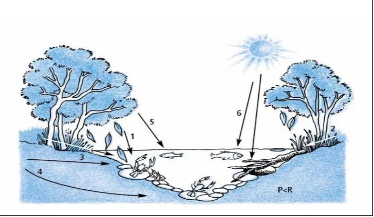
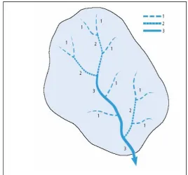
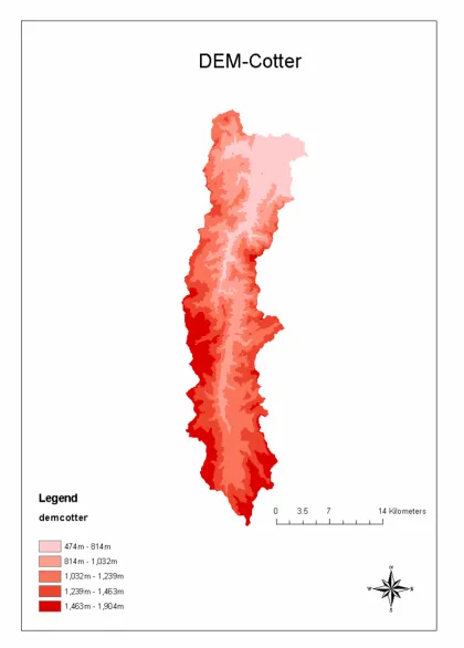
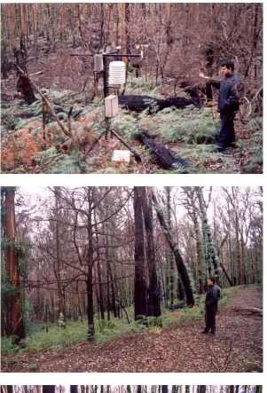
(11) List of Figures. Figure 1.1: Conceptual model of the global carbon (above) and water (below) cycles…….4 Figure 1.2: The carbon compartments of a terrestrial ecosystem (carbon dynamics)………5 Figure 2.1: Sources of organic carbon inputs to forested rivers……………………………19 Figure 2.2: A schematic model showing the relationship between stream order differences and position in landscape………………………………………………………………………..21 Figure 2.3: The relationship among the contributed chapters showing the methodology adopted in the Cotter River Catchment …………………………………………….…….................25 Figure 3.1: Location of the Cotter River Catchment in the Murrumbidgee Catchment and Australia…………………………………………………………………………………….28 Figure 3.2: Cotter River Catchment and its three sub-catchments (Corin, Bendora, and Lower Cotter) in the ACT………………………………………………………………………….29 Figure 3.3: Location of climate and flow stations in the Cotter River Catchment………...35 Figure 3.4: Annual average of potential evaporation and rainfall in the Cotter River Catchment……..……………………………………………………………………………36 Figure 3.5: Long-term mean maximum temperature data from January to December in the Cotter River Catchment…………………………………………………………………….37 Figure 3.6: Long-term mean minimum temperature data from January to December in the Cotter River Catchment…………………………………………………………………….39 Figure 3.7: High resolution (20 meter) Digital Elevation Model (DEM) data representing the topography of the Cotter River Catchment…………………………………………………40 Figure 3.8: Cotter River Catchment Vegetation Map based on different communities…………………………………………..…………………………………….44 Figure 3.9: Soil group classification of the Cotter River Catchment……………………….48 Figure 3.10: Map of Wildfire history in the ACT and Major Bushfires since 1920………..52 Figure 3.11: Impacts of wildfires 2003 on the Cotter River Catchment and ACT derived from Landsat 7 ETM+, 7 November 2002 (before) and 26 January 2003 (after) the wildfire…..53 Figure 3.12: Bushfire seasons in Australia…………………………………………………54 Figure 3.13: Understorey cover post the 2003 wildfire, Warks Road (Lower Cotter Catchment)………………………………………………………………….62 Figure 3.14: Cotter River Catchment at New Chums Road showing affected area………..63 Figure 3.15: Cotter Catchment at Warks Road, before the Namadgi National Park Boundary…………………………………………………………………………………....64. xi.

(12) Figure 3.16: Impacts of wildfire on Cotter River Catchment………………………………65 Figure 4.1: Flow networks and their connected regions in the Cotter River Catchment…………………………………………………………………………………..72 Figure 4.2: Schematic diagram of the IHACRES rainfall-runoff model showing components…………………………………………………………………………………74 Figure 4.3: Simplified data transfer and spatial process framework used to produce catchment attributes in the Cotter River Catchment…………………………………………………...85 Figure 4.4: GIS Layers produced through spatial analysis in the Cotter River Catchment…………………………………………………………………………………..85 Figure 4.5: The seven combined sub-catchment areas generated through spatial analysis in the Cotter River Catchment…………………………………………………………………….88 Figure 4.6: Observed and modelled flow duration curves for model calibration period at gauge number 410730 with calibration R2 = 0.70, gauge number 410733 with calibration R2 = 0.68, and gauge number 410776 with calibration R2 = 0.77………..…………………………….93 Figure 4.7: IHACRES calibration result for gauge number 410730. Modelled, observed, slowflow and residual flows are plotted (Calibration R2 = 0.70)………………………………..94 Figure 4.8: IHACRES calibration result for gauge number 410733. Modelled, observed, slowflow and residual flows are plotted (Calibration R2 = 0.68)………………………………..95 Figure 4.9: IHACRES calibration result for gauge number 410776. Modelled, observed, slowflow and residual flows are plotted (Calibration R2 = 0.77)………………………………..96 Figure 4.10: Observed and modelled flow duration curves for model simulation period at Gingera, Coree, and Licking Hole Creeks (three gauges) of the Cotter River Catchment…98 Figure 4.11: IHACRES simulation result for gauge 410730. Observed and modelled, slow-flow, and residual flows are plotted. Simulation R2 = 0.66………………………………………99 Figure 4.12: IHACRES simulation result for gauge 410733. Observed and modelled, slow-flow, and residual flows are plotted. Simulation R2 = 0.71………………………………………100 Figure 4.13: IHACRES simulation result for gauge 410776. Observed and modelled, slow-flow, and residual flows are plotted. Simulation R2 = 0.81………………………………………101 Figure 4.14: A schematic diagram of watershed delineation to generate the 75 sub-catchment areas in the Cotter River Catchment……………………………………………………......105 Figure 4.15: The 75 merged sub-catchment areas produced through watershed delineation used for regionalization method in the Cotter River Catchment…………………………………108 Figure 4.16: Seven combined sub-catchment areas (sampling sites) produced in the Cotter River Catchment…………………………………………………………………………………..109 Figure 4.17: Unit Hydrograph in Gingera Creek revealing half peak flow (Hw = 0.34)…………………………………………………………………………………119. xii.

(13) Figure 4.18: Unit Hydrograph in Coree Creek revealing half peak flow (Hw = 0.27)…………………………………………………………………………………119 Figure 4.19: Unit Hydrograph in Licking Hole Creek revealing half peak flow (Hw = 0.28)…………………………………………………………………………………119 Figure 4.20: Simulation results at seven sampling sites (ungauged locations) estimated through regionalization approach in the Cotter River Catchment from May 1967 to July 2004…………………………………………………………...124-126 Figure 4.21: Observed, regionalized and calibrated flow duration curves for the calibration period at gauge number 410733 (Coree Creek) …………………………………………....126 Figure 5.1: Sampling sites and their connected regions in the Cotter River Catchment……………………………………………………………………………130 Figure 5.2: Map of organic carbon sampling sites in the Cotter River Catchment………...143 Figure 5.3: Simulated streamflow discharge estimated through IHACRES simulation model in the seven sampling sites of Cotter River Catchment for entire time period (May 1967 – July 2004) and sampling period (July 2003 – June 2004)…………………………………..152-154 Figure 5.4: Correlation between carbon concentration and streamflow for the sampling sites Blundells and Collins Creek………………………………………………………………...159 Figure 6.1: The various stages involved in processing the time series, from data ordering to NDVI outputs through ERDAS IMAGINE 8.6…………………………………………….181 Figure 6.2: Flowchart of the analytic process involved in the conversion of NDVI time series to fAPAR time series in the Cotter River Catchment…………………………………………183 Figure 6.3: Minimum and maximum accumulated (multiplied by 10000) image of NDVI time series values for each pixel of the relevant tile h30v12 used for NDVI conversion to Fi (Cotter River Catchment is represented as a green grid)…………………………………………...185 Figure 6.4: ERDAS IMAGINE File Information, showing the distribution of minimum NDVI values (multiplied by 10000)……………………………………………………………….186 Figure 6.5: ERDAS IMAGINE File Information, showing the distribution of maximum NDVI VALUES (multiplied by 10000)……………………………………………………………187 Figure 6.6: A schematic graph representing the relationship between NDVI and Fi (fAPAR) in the Cotter River Catchment…………………………………………………………………188 Figure 6.7: Distribution of minimum, maximum, and average monthly short-wave radiation (RS) estimated by SRAD and ESOCLIM from January to December using 20m DEM in the Cotter River Catchment……………………………………………………………………………206 Figure 6.8: Distribution of minimum, maximum, and average monthly light use efficiency ( ε ) estimated from January to December in the Cotter River Catchment..........................207 Figure 6.9: Distribution of GPP values (mol C m-2 month-1) estimated from July 2003 to June 2004 in the seven sampling sites…………………………………………………………...213. xiii.

(14) Figure 6.10: Distribution of GPP and NPP values (mol C m-2 month-1) estimated from December 2001 to August 2004 in the Cotter River Catchment consisting of the wildfire of January 2003 and the sampling period used in this case study (July 2003 – June 2004)…………………217 Figure 6.11: GPP values (mol C m-2 year-1) estimated from July 2003 to June 2004 in the 75 sub-catchments of the Cotter River Catchment…………………………………………….218 Figure 6.12 Annual NPP (g C m-2 year-1) estimated through 12 models and a mean value as the average of all models estimates in comparison with current method’s output (No. 13 – above) used in the Cotter River Catchment………………………………………………………...223 Figure 7.1: Cross Correlation analysis between GPP and DOC in the five sampling sites of the Cotter River Catchment showing a time lag (month) ………………..…………………….230 Figure 7.2: Cross Correlation analysis between GPP and POC in the five sampling sites of the Cotter River Catchment showing a time lag (month)………………………………………231 Figure 7.3: Cross Correlation analysis between GPP and TOC in the five sampling sites of the Cotter River Catchment showing a time lag (month)………………………………………232 Figure 7.4: Cross Correlation analysis between GPP and Load-DOC in the five sampling sites of the Cotter River Catchment representing a time lag (month) ……………………………...238 Figure 7.5: Cross Correlation analysis between GPP and Load-POC in the five sampling sites of the Cotter River Catchment representing a time lag (month)... ……………………………239 Figure 7.6: Cross Correlation analysis between GPP and Load-TOC in the five sampling sites of the Cotter River Catchment representing a time lag (month) ……………………………...240 Figure 7.7: Regression coefficients a and b plotted against the percentage of high affected areas in the five sampling sites of Cotter River Catchment. The linear regression line fitted to this data is also shown ……………………………………………………………………………….246 Figure 7.8: The variation of GPP, Flow, TOC and TOC Load across the 75 sub-catchments of the Cotter River Catchment during July 2003 – June 2004………………………………...253 Figure 7.9: The variation of TOC Load/GPP (%) across the 75 sub-catchments of the Cotter River Catchment during July 2003 – June 2004 (the 75 sub-catchments are shown from x1 to x75)……………………………………………………………………………………........253 Figure 7.10: The distribution of mean GPP values (Tonnes/km2year-1) between July 2003 and June 2004 in the Cotter River Catchment……………………………..……………………254 Figure 7.11: The distribution of mean TOC Load values (Tonnes/km2 year-1) between July 2003 and June 2004 in the Cotter River Catchment...……………………………………………255 Figure 7.12: Carbon flux dynamics for the Cotter River Catchment based on data and analyses for the period July 2003 – June 2004………………………………………………………258. xiv.

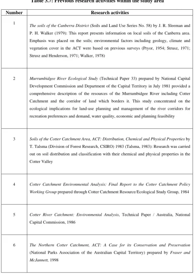
(15) List of Tables Table 3.1: Sources of the hydrologic (ID: Prefix 410) and climatic (ID: Prefix 570) point time series data set in the Cotter River Catchment ...........................................…………………33 Table 3.2: Average Maximum temperature data from January to December in the Cotter River Catchment…………………………………………………………………………………..38 Table 3.3: Average Minimum temperature data from January to December in the Cotter River Catchment…………………………………………………………………………………..38 Table 3.4: Fire Severity in the ACT and Cotter River Catchment based on Severity Analysis tested in this research…………………………………………………….............................42 Table 3.5: Classification of vegetation communities in the Cotter River Catchment…………………………………………………………………………………..43 Table 3.6: The percentage burnt of each of the important Wetlands in the Cotter River Catchment areas…………………………………………………………………………….59 Table 3.7: Previous research activities within the study area……………..………………..66 Table 4.1: IHACRES model parameters (non-linear and linear module)………………….77 Table 4.2: Maps and data sources required for the program……………………………….78 Table 4.3: A summary of catchment attributes for the seven sub-catchments investigated in the Cotter River Catchment (Gauged Locations)……………………………………………....86 Table 4.4: A summary of catchment attributes for the seven sampling sites investigated in the Cotter River Catchment (Ungauged Locations)……………………………………………87 Table 4.5: Rainfall-Runoff (IHACRES) model parameters (Non-Linear and Linear) and calibration results for three gauges in the Cotter River Catchment………………………...91 Table 4.6: IHACRES model simulation results for three gauges in the Cotter River Catchment…………………………………………………………………………………..97 Table 4.7: Catchment attributes for each of the 75 sub-catchment areas generated during regionalization method in the Cotter River Catchment…………………………………….106 Table 4.8: Estimated runoff coefficient for three gauges in the Cotter River Catchment to obtain adjusted g(m)……………………………………………………………………………….114 Table 4.9: Estimated runoff coefficient in the ungauged locations (75 sub-catchments + 7 sampling sites) of Cotter River Catchment…………………………………………………114 Table 4.10: Estimated (half peak flow) for three gauges of the Cotter River Catchment…………………………………………………………………………………..118 Table 4.11: Model parameters estimated through regionalization method in the 75 subcatchments and seven sampling sites (ungauged locations) of the Cotter River Catchment…………………………………………………………………………………..122. xv.

(16) Table 5.1: Seven points selected for sampling program in the Cotter River Catchment…………………………………………………………………………………..142 Table 5.2: Organic Carbon data collected through sampling program in the Cotter River Catchment…………………………………………………………………………………..146 Table 5.3: Integrated monthly streamflow data for seven sampling sites between July 2003 and June 2004 in the Cotter River Catchment…………………………………………………..151 Table 5.4: Estimated organic carbon loads for five sub-catchments of Cotter River Catchment between July 2003 and June 2004………………………………………………………….156 Table 6.1: Average daily solar irradiance at the top of the atmosphere for each month (MJ m2 d-1) in the Cotter River Catchment…………………………………………………190 Table 6.2: Average daily solar irradiance at the top of the atmosphere for each month (MJ m2 d-1) at different Latitudes…………………………………………………………...191 Table 6.3: SRAD parameter values for calculating short-wave irradiance in the Cotter River Catchment…………………………………………………………………………………..197 Table 6.4: SRAD Solar Declination values in different months of the year in the Cotter River Catchment…………………………………………………………………………………..199 Table 6.5: SRAD sunshine fraction and transmittance values of Cotter River Catchment in different months of the year………………………………………………………………...199 Table 6.6: Detailed a SRAD parameter file (srad_param)………………………………….201 Table 6.7: Input parameters file for SRAD calculation…………………………………….202 Table 6.8: Modified time step used for calculating RS in different month of year through additional input parameters for SRAD……………………………………………………..203 Table 6.9: A comparison of RS (M J m-2) between SRAD results and ESOCLIM products in the Cotter River Catchment…………………………………………………………………….205 Table 6.10: Monthly average of ε (mol CO2 mol-1 PAR) calculated in the Cotter River Catchment…………………………………………………………………………………..207 Table 6.11: Vegetation productivity values (g C m-2 year-1) using the TMS method for different vegetation classes (T and MS) of Cotter area………………………………………………211 Table 6.12: Monthly average of GPP (mol C m-2) estimates in the seven sampling sites of Cotter River Catchment from July 2003 to June 2004…………………………………………….212 Table 6.13: Monthly average of GPP (g C m-2) estimates in the seven sampling sites of Cotter River Catchment from July 2003 to June 2004…………………………………………….212 Table 6.14: Monthly GPP (Tonnes/area) calculates in the seven sampling sites from July 2003 to June 2004………………………………………………………………………………...215 Table 6.15: Monthly average of GPP and NPP estimates from December 2001 to August 2004 in the Cotter River Catchment……………………………………………………………...216. xvi.

(17) Table 6.16: Annual GPP estimates in the 75 sub-catchments during sampling period July 2003 – June 2004…………………………………………………………………………...219 Table 6.17: A comparison between results for 12 models of NPP estimation and the radiation use efficiency approach used in the Cotter River Catchment………………………………222 Table 7.1: Regression analysis between GPP and DOC in the five sampling locations of Cotter River Catchment from July 2003 to June 2004…..…………………………………………233 Table 7.2: Regression analysis between GPP and POC in the five sampling locations of Cotter River Catchment from July 2003 to June 2004……………………………………………..233 Table 7.3: Regression analysis between GPP and TOC in the five sampling locations of Cotter River Catchment from July 2003 to June 2004..……………………………………………234 Table 7.4: Regression analysis between GPP and DOC loads in the five sampling sites of Cotter River Catchment from July 2003 to June 2004……………………………………………..241 Table 7.5: Regression analysis between GPP and POC loads in the five sampling sites of Cotter River Catchment from July 2003 to June 2004……………………………………………..242 Table 7.6: Regression analysis between GPP and TOC loads in the five sampling sites of Cotter River Catchment from July 2003 to June 2004……………………………………………..243 Table 7.7: The percentage of fire impact estimated in the five sampling sites of Cotter River Catchment…………………………………………………………………………………..245 Table 7.8: The data set used for generating regression relationships based on wildfire impacts in the Cotter River Catchment………………………………………………………………...245 Table 7.9: The data set used for generating two regression relationships based on wildfire impacts in the 75 sub-catchments of Cotter River Catchment……………………………..248 Table 7.10: The final comparison between GPP and TOC Load values in the 75 sub-catchment areas of Cotter River Catchment during July 2003 – June 2004…………………………...251. xvii.

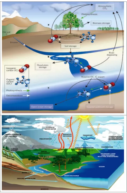
(18) List of Appendices. Appendix 4.1: Streamflow results in the 75 sub-catchments area of the Cotter River Catchment between July 2003 and June 2004.. 318. Appendix 5.1: Organic carbon and streamflow data collected at the seven sampling sites...320 Appendix 6.1: NDVI conversion to fAPAR between December 2001 and August 2004 for the Cotter River Catchment. 324. Appendix 6.2: Daily results of the solar radiation at the top of the atmosphere (RO) calculated for the Cotter River Catchment. 357. Appendix 6.3: The monthly comparison results of the solar radiation at the top of the canopy (RS) (MJm-2) estimated between ESOCLIM (left) and SRAD (right) for the Cotter River Catchment. 369. Appendix 6.4: Monthly spatial distribution of light use efficiency ( ε ) (mol CO2 mol-1 PAR) calculated for the Cotter River Catchment. 381. Appendix 6.5: The annual NPP (gCm-2) estimation derived from 12 models and corresponding ranges calculated for the Cotter River Catchment. 393. Appendix 7.1: The regression analysis between GPP and DOC, POC, TOC in the sampling sites of the Cotter River Catchment. 405. xviii.

(19) Chapter One Introduction. 1.1 Global carbon and water cycle The increase in atmospheric CO2 concentrations and the associated effects on the global climate have catalyzed the need for improved understanding of the carbon cycle (Robertson et al., 1996; Aumont et al., 2001). For the heterogeneous land surface, spatially explicit carbon budgets are required for defining and implementing mitigation policies such as those under the Kyoto protocol, and to make predictions of global change more reliable. The focus of this study is the role of hydrology in the carbon budget in terms of organic carbon fluxes at the catchment scale. Carbon is stored on our planet in several major sinks: (1) as the gas Carbon Dioxide (CO2) in the atmosphere; (2) in terrestrial ecosystems (living-dead biomass and soil); (3) fossil fuels and sedimentary rocks in the lithosphere; (4) the ocean carbon stocks and calcium carbonate in marine organisms (Pidwirny, 2000). Soil carbon is a major component of the global inventory and exerts significant influence on carbon dynamics in connection with changes in climate and human land use (Schimel et al., 1994). Soil organic carbon comprises approximately two-thirds of terrestrial carbon storage (Schimel et al., 1994). It has been proposed that soil carbon plays a significant role as a source (Schimel et al., 1990; Townsend et al., 1992) or sink (Tans et al., 1990; Harrison et al., 1993) of carbon dynamics in response to climate changes and atmospheric CO2.. In dry mass terms, carbon is the major constituent of all living ecosystems and is highly abundant in the atmosphere, water and soil. Through oxidation and reduction reactions, the cycling of other elements is closely connected to the global cycle of carbon. Carbon is therefore a key focus when studying the factors that influence organic matter production and turnover in ecosystems (Robertson et al., 1996). Water, organic carbon and other chemical substances in hydrological processes are connected through ecosystem processes and are strongly influenced by climate. Human activities have also profoundly affected hydrologic processes and nutrient cycling in terrestrial and freshwater aquatic ecosystems (Gallowag et al., 1995). Land cover changes affect hydrological processes and these changes interact with organic carbon and nutrients in many significant ways. For instance,. 1.

(20) land use and land management activities affect the hydrological response of a system and thus nutrient fluxes through changes in land cover, evapotranspiration, and soil characteristics. These changes are followed by feedback mechanisms among water, carbon and other chemical substances that bring further changes in these linked processes (Alexander and Smith, 1990).. The terrestrial carbon cycle has so far been studied mainly from the ecological-biogeochemical and atmospheric perspectives (Wood et al., 2002) and has largely ignored the hydrological flux of organic carbon (Goldewijk et al., 1994). Recent studies on river ecosystems have shown that river discharge, primary production and litter pool sizes in watersheds and the development of agriculture in catchments are major processes that influence the fluxes of organic carbon in rivers (Robertson et al., 1996). Other studies have proposed that this is an important lateral process that may constitute a significant stock and flux of organic carbon at catchment scale (Sarin et al., 2002). There are still major deficiencies in knowledge of the sources, transformation and cycling of organic carbon in river environments (Robertson et al., 1996). A review by Robertson et al. (1996) revealed three main categories of factors that govern organic carbon fluxes in catchments:. 1) Streamflow: Variation in streamflow is the major controlling factor in the supply of carbon from catchments to the river channel. It is also a key factor controlling the rates, forms and distribution of primary production in the catchment and river channel (Robertson et al., 1996). However, the relationship between flow variations and the delivery of dissolved organic carbon (DOC) and particulate organic carbon (POC) through the river systems is poorly understood.. 2) Land Management: Land management practices play a central role in determining the forms and quantities of carbon that are entered in rivers. The combination of clearing, soil compaction and changes in vegetation types alters the quantities, types, quality and pathways of carbon entering catchment areas of rivers (Robertson et al. 1996). These effects can be considered more generally in terms of land use and land cover changes, which can be due to land management or natural disturbances such as wildfire.. 3) Quality of carbon: The majority of the carbon being transported in rivers is likely to be highly refractory (Robertson et al., 1996). Recent studies show that a very small fraction of the total carbon transported in rivers is labile and that this supports the majority of oxidative processes and the food chains (Robertson et al., 1996). The relative concentrations of carbon and other nutrients in organic matter have a strong impact on carbon fluxes. The total pool of organic carbon (TOC). 2.

(21) therefore includes particulate organic carbon (POC) and dissolved organic carbon (DOC). This combined pool contains carbon from autochthonous (in-stream) sources and allochthonous (offstream) sources. The hydrological flux of organic carbon can be understood through measuring the production and transformation of carbon in the contributing catchments (off-stream) and studying the in-stream processing of carbon.. Changes in organic carbon and other chemical substances of fluxes are connected to changes in hydrological processes in river systems, land cover patterns and vegetation. Changes in C, N, and P fluxes in turn induce further changes in the hydrological process itself, which can have adverse or positive impacts on terrestrial and aquatic resources. Anticipating these changes and impacts requires a fundamental understanding of the links between the carbon and hydrological fluxes in terrestrial and inland aquatic systems found within a water catchment.. The study of the transport of organic carbon through the world’s streams and rivers provides information on the rate of erosion of continents, the cycling of carbon on Earth, and the contribution of terrestrial carbon to the aquatic systems and oceans (Meybeck, 1982; Meybeck, 1993; Robertson et al., 1996; Sarin et al., 2002; Peel et al., 2003). The transportation of organic carbon from terrestrial ecosystems by rivers and hydrological fluxes to the oceans plays important roles in regional budgets of organic carbon entering the continent-ocean interface (Sarin et al., 2002). The flux of hydrological organic carbon has been found to correlate with environmental variables such as edaphic, climatic, topographic, ecologic and hydrological processes (Meybeck, 1993; Robertson et al., 1996; Lovett and Price, 1999; Meybeck and Vorosmarty, 1999; Neff and Asner, 2001; Raymond and Bauer, 2001; Sarin et al., 2002). These processes constitute natural controls on carbon flux in rivers and include organic carbon sequestration by plants and environmental controls on gross primary productivity (GPP) / net primary productivity (NPP), and the water balance. The main stocks and fluxes of the global carbon and water cycle are shown in Figure 1.1. This figure illustrates how GPP occurs in streams through aquatic photosynthesising, and how streams also receive organic carbon input from vegetation in the surrounding catchment. In the global carbon cycle, photosynthesis in land plants fixes atmospheric CO2 (inorganic carbon) as organic carbon (phase a). This process can be followed in rivers through decomposition and photosynthesis (phase b). The process continues in the oceans (phase c).. 3.

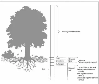
(22) Figure 1.1: Conceptual model of the global carbon (above) and water (below) cycles Source: Water Cycle Study Group, 2001; Raymond, 2005. 4.

(23) Surface runoff (see Figure 1.1) can be used to assess the impacts of land use, land cover, atmospheric deposition, hydrological variations and climatic differences on the hydrologic flux of organic carbon across the catchment. Data on surface water quality (including DOC and POC) provide a spatially integrated sample of organic carbon (DOC and POC) that is likely to reveal catchment conditions as an output net carbon flux.. A major source of organic carbon (DOC and POC) is the carbon pools of the terrestrial biosphere (Esser and Kohlmaire, 1989; Bauer and Druffel, 1998). These pools consist of living biomass (aboveground biomass), dead biomass (litter) and soil organic carbon (SOC) largely resulting from litter (WBGU, 1998). Figure 1.2 shows the carbon compartments of a terrestrial ecosystem (carbon dynamics). This Figure can be compared with the components presented in Figure 1.1.. Figure 1.2: The carbon compartments of a terrestrial ecosystem (carbon dynamics) Source: WBGU, 1998. 5.

No results found