Dynamic Optimization of a Rimless Wheel with an Actuated Pendulum

(1)

Theses Thesis/Dissertation Collections

8-2015

Dynamic Optimization of a Rimless Wheel with an

Actuated Pendulum

Benjamin Thomas Mihevc

Follow this and additional works at:http://scholarworks.rit.edu/theses

This Thesis is brought to you for free and open access by the Thesis/Dissertation Collections at RIT Scholar Works. It has been accepted for inclusion in Theses by an authorized administrator of RIT Scholar Works. For more information, please [email protected].

Recommended Citation

(2)

Wheel with an Actuated Pendulum

by

Benjamin Thomas Mihevc

A Thesis Submitted in Partial Fulfillment of the Requirements for the Degree of Master of Science

in Computer Engineering

Supervised by

Juan C. Cockburn

Department of Computer Engineering Kate Gleason College of Engineering

Rochester Institute of Technology Rochester, New York

August 2015

Approved by:

Juan C. Cockburn, Associate Professor

Thesis Advisor, Department of Computer Engineering

Mario W. Gomes, Assistant Professor

Co-advisor, Department of Mechanical Engineering

Agamemnon L. Crassidis, Associate Professor

Committee Member, Department of Mechanical Engineering

Andres Kwasinski, Associate Professor

(3)

Abstract

Dynamic Optimization of a Rimless Wheel with an Actuated Pendulum

Benjamin Thomas Mihevc

As the demand for mobile robots that work alongside humans increases,

the amount of energy that these co-robots consume will become a critical

limiting factor in their deployment. This need is clearly captured in one

of the fifteen main goals of the 2009 Roadmap for US Robotics which is to

create a robot that can walk with half the energy consumption of a human

being. At this point, the most energy-efficient walking robot is about as

energy efficient as a human.

Energy efficient bipedal motion is an active area of research. It has been

proven that it is theoretically possible to design a robot with intermittent

support, one of the most fundamental attributes of legged locomotion, to

have a zero-energy cost collisionless gait.

Optimal control has been used by a number of researchers to study the

generation of periodic gaits for walking robots. However little research

exists demonstrating walkers with energy efficient collisionless motion.

(4)

the energy lost to the system when walking is from losses due to step

col-lisions.

In this work energy efficient locomotion of a prototype actuated rimless

wheel on level ground is explored using numerical optimal control. The

actuated rimless wheel has an internal pendulum driven by a DC motor.

The locomotion problem is posed as an optimal control problem.

Dif-ferent cost functions and initial configurations are investigated and the

corresponding gait trajectories analyzed and assessed based on their use

of energy and the potential for collisionless motion.

The results of this work will provide the foundation for the design and

im-plementation of more energy efficient actuated rimless wheel prototype

(5)

List of Figures

1.1 Diagram of a Rimless Wheel . . . 2

3.1 Diagram of a Pendulum Coupled Rimless Wheel . . . 10

3.2 Free Body Diagrams of the Pendulum Coupled Rimless Wheel 10 3.3 Generalized Circuit of DC Motor . . . 22

3.4 System Before (Left) and After (Right) an Instantaneous Col-lision . . . 24

4.1 Single Colliding Step with Voltage Cost . . . 43

4.2 Single Colliding Step with a Multi State Cost . . . 44

4.3 Single Colliding Step Energy . . . 45

4.4 Single Collisionless Step . . . 47

4.5 Single Collisionless Step Simulation Verification . . . 48

4.6 Single Collisionless Step Energy . . . 49

4.7 Two Colliding Steps with Low Wheel Position Cost . . . 54

(8)

4.10 Two Colliding Steps with Low Wheel Costs . . . 57

4.11 Two Colliding Steps with Low Wheel Costs Verification . . . . 57

4.12 Two Colliding Steps with Low Wheel Costs Energy . . . 58

4.13 Two Colliding Steps with Low Position Costs . . . 59

4.14 Two Colliding Steps with Low Position Costs Verification . . . 60

4.15 Two Colliding Steps with Low Position Costs Energy . . . 61

4.16 Two Colliding Steps with High Wheel Velocity Cost . . . 62

4.17 Two Colliding Steps with High Wheel Velocity Cost

Verifica-tion . . . 63

4.18 Two Colliding Steps with High Wheel Velocity Cost Energy . . 64

4.19 Two Colliding Steps with High Wheel Velocity Cost . . . 65

4.22 Three Colliding Steps GPOPS-II . . . 68

4.25 Two Steps Collision Dynamics GPOPS-II . . . 74

(9)

4.28 Single Step Extension to Multi-Step Result, Experiment 1 . . 77

4.31 First Single Step Extension to Multi-Step Result, Experiment 5 80

4.32 Second Single Step Extension to Multi-Step Result,

Experi-ment 5 . . . 81

4.33 Single Step Extension to Multi-Step Verification, Experiment

1 . . . 81

(10)

List of Tables

1 List of Variables . . . x

4.1 Nominal Parameter Values . . . 37

4.2 Motor Parameters . . . 37

4.3 Experiment 1 State Constraints . . . 41

4.6 Physical Parameter Values . . . 71

(11)

[image:11.612.112.505.218.547.2]

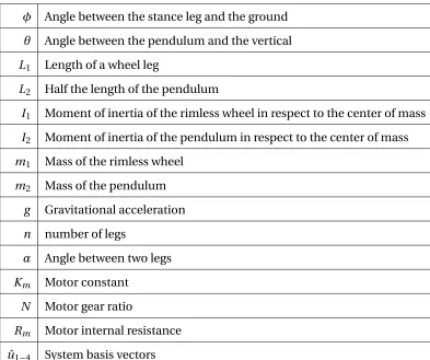
List of Variables

Table 1: List of Variables

φ Angle between the stance leg and the ground

θ Angle between the pendulum and the vertical

L1 Length of a wheel leg

L2 Half the length of the pendulum

I1 Moment of inertia of the rimless wheel in respect to the center of mass

I2 Moment of inertia of the pendulum in respect to the center of mass

m1 Mass of the rimless wheel

m2 Mass of the pendulum

g Gravitational acceleration

n number of legs

α Angle between two legs

Km Motor constant

N Motor gear ratio

Rm Motor internal resistance

ˆ

(12)

Chapter 1

Introduction

Numerical optimization is a tool that allows for the determination of an

ideal solution based on a cost criteria. This cost must be minimized to

find this optimal solution. To minimize this cost, function inputs are

al-tered based on the first and second derivatives of the system until an

op-timal solution is found. This is the fundamental idea that opop-timal control

is built upon.

Optimal control is an extension of numerical optimization. With optimal

control, the cost is often a function of functions and the input is a set of

trajectories instead of a constant. The system is then subject to a

num-ber of dynamic constraints. Then, by varying the input trajectories, an

optimal set of state trajectories can be determined.

Optimal control can be, and often is, applied to energy minimization

prob-lems. By using several of the components of the energy in the system as

a cost function, inputs can be found that minimize energy use. However,

it must be noted that optimization is based on a cost function. If the cost

(13)

an actual optimal solution may not be found.

Why is energy efficient optimal control important ? The answer to that

question changes constantly. In the 1950s, it was important to enable the

efficient use of rockets for space travel. In the 1960s, it was important

for developing optimal climb trajectories for high performance military

aircraft. Today, it is important for efficient robotic motion.

Historically, robotic walkers started out focused on statically stable

mo-tion. Though practical for early research, maintaining constant stability

is not energy efficient. Proceeding from stable gaits to half stable and

periodic gaits was the focus of much of the early 1990s through the early

2000s. During this research, the rimless wheel was developed. This wheel,

seen in Figure 1.1, can be likened to a wagon wheel with the wheel part removed. This leaves only the spokes.

φ

L1

Figure 1.1: Diagram of a Rimless Wheel

(14)

focused on the creation and simulation of an energy efficient walker

ca-pable of level ground transport. The goal was to reduce the energy of

transport by generating collision free motion. For his research, a five

legged walker with an internal inertial device was created. The inertial

device consisted of a torsional spring attached to a rotating mass.

In simulation, frictional losses prevented the passive system from

achiev-ing collisionless motion. Attempts to apply simple actuation and

feed-back control to the system did improve the cost of transport, but did not

reintroduce collisionless motion [1].

In this thesis this problem will be reexamined using optimal control. To

apply optimal control to the system, an understanding of the dynamics of

the rimless wheel must obtained. First studied in detail by McGeer in the

late 1980s and early 1990s, the rimless wheel is considered the simplest

walking system [2]. It has been shown to be a half stable, 1-period system

when walking down an incline. When walking on level ground the system

is asymptotically stable [3].

Rimless wheels with actuation have been proposed and implemented to

further gain insight into collisionless motion. Among the many

actua-tion methods the most common are telescoping legs, spinning inertial

devices, and wobbling pendulums. Most of these methods of actuation

sought a stable gait frequency.

(15)

walking rimless wheel. We will consider the minimization of the control

effort as a surrogate to input energy, but we will also seek to determine

the optimal trajectory that leads to a collisionless step.

We will begin by deriving the dynamics of the system and the equations

of motion. From there, a simulation of the system will be developed.

Fol-lowing that, the optimal control problem will be formulated and solved

for various wheel configurations with various costs functions. We will

ex-periment with penalizing state movement and control input. Finally we

will analyze our results and discus physical implementation of the

(16)

Chapter 2

Literature Review

In the late 1980s and early 1990s, McGeer pioneered passive dynamic

walking by introducing the rimless wheel [2]. The dynamics of the

less wheel were studied significantly. Since the introduction of the

rim-less wheel it’s passive stability on a gentle incline was determined to be

1-period half stable. With frictional losses, the system is asymptotically

stable [4][5][3][6].

Gamus and Or [6] examined the dynamic legged locomotion of a robotic

walker that undergoes a constant falling motion followed by foot

place-ment. Their work involved a rimless walking wheel without any kind of

secondary oscillation or actuated swinging body besides the wheel itself.

In the paper, they examine the slipping dynamics of the wheel. Though

beyond the scope of my research, the dynamics of their walker are similar

to the simplified dynamics of the walker we are describing.

Passive walking wheels provide a simple way to model stepping motions,

but do not have any inherent methods of actuation. Generating a walking

(17)

to these systems are numerous. Some of the more popular methods

in-clude telescoping legs [7], external actuated torsos [5][8], virtual slopes

generated by an actuated heel [9], wobbling pendulums [10], small

phys-ical slopes [1], and many more.

Fumihiko Asano created a passive dynamic walking rimless wheel with a

two degree of freedom wobbling mass on the center of mass of the wheel

[10]. This walker was shown to demonstrate the effect of a passive

wob-bling mass on a walker moving down an incline. The wobwob-bling mass

swings on a pin joint at the center of the wheel’s mass and telescopes

along the pendulum arm’s length. If the telescoping arm’s length is held

constant, the walker is essentially the one in this thesis.

Asano used this walker to demonstrate the asymptotically stable gait of

this type of walker. In addition, the swinging of the inner mass was used

as a controller to achieve a reference frequency. Asano was able to

demon-strate that this type of walker is capable of achieving a controlled gait for

high efficiency movement using simple PID control while walking down

a negative slope [10].

Much of the research involving rimless wheels is foundational work that

leads directly to bipedal walking [6] [3] [7] [5]. These bipedal walkers

al-most exclusively focus on stable periodic walking gaits.

Walkers that can achieve stable periodic bipedal motion need to be

(18)

the center of mass of the robot to allow for dynamic motion. In their work,

they model their robot as an inverted double pendulum that has an upper

mass and a swinging foot. By altering the center of mass of their system

they were able to achieve a more efficient method of robotic locomotion.

A Lagrangian approach was used to determine the equations of motion

of the rimless wheel. General background on this approach can be found

in [12] and [13].

Efficient robotic locomotion yields directly to optimal control. Numerous

authors have used optimal control for bipedal and rimless wheel walkers

[14] [15] [16] [17] [18] [19] [20] [21] [22]. Where most of the work involving

optimal control and walking robots differ are the actuation methods. In

general, the cost function of the optimal control problem is either gait

frequency or energy, or both. In some cases, electrical input energy and

storing the systems kinetic energy prior to a step is considered [19], but

the energy lost in the collision with the ground is rarely studied.

As was discovered by Ahlin [1] and previously discussed, a significant

amount of energy is lost in foot collisions. Determining if a trajectory

ex-ists that can yield actuated collisionless motion is of significant interest.

The locomotion problem was formulated as an optimal control problem.

For background on optimal control and dynamic optimization see [23]

[24] [25] [26]. The optimal control problem was then solved numerically

(19)

multiple-phase optimal control problems using Gaussian pseudospectral

methods is based on research by Rao et al. [27]. This method discretizes

the problem as approximations of the states and control using high order

polynomials [27] [28] [29]. The coefficients of the polynomials can then

be solved for using traditional optimization methods. This "collocation”

of the system is dynamic in nature and does not require a constant

(20)

Chapter 3

The Actuated Rimless Wheel

This section describes the dynamics of a rimless wheel system. In it the

equations of motion, energy equations, and control torque equations will

be presented and explained. Additionally, the derivations will be

pre-sented in detail. The relevant free body diagrams will be prepre-sented and

their significance will be explained.

3.1 Newton-Euler Equations

The rimless wheel dynamics will be described as a double pendulum.

This system is a system with two pin joints, one being the motionless

pivot joint on the ground, and the other being the moving pivot at the

center of gravity of the rimless wheel. This can be seen in Figure3.1where φ is the angle between the spoke and the ground and θ is the angle

be-tween the vertical axes and the inner pendulum’s arm.

This system can be split into two separate free body diagrams. These free

(21)

φ

θ

L1

L2

ψ

Figure 3.1: Diagram of a Pendulum Coupled Rimless Wheel

acting on the outer wheel of this system. In the simulation, this system

acts as the first arm of the double pendulum. System 2 is describes the

forces acting on the inner arm of the pendulum. System 1 in Figure 3.2

φ

θ Ry

Rx

m1g τ

m2g Rx

Ry

ˆ

u2

ˆ

u1 ˆ

u4

ˆ

u3

ˆ



ˆı

ˆ



ˆı

System 1 System 2

τ

o

Fy

Fx

Figure 3.2: Free Body Diagrams of the Pendulum Coupled Rimless Wheel

introduces two coordinate axis. The first axis is the standard ˆı, ˆ, and ˆk

coordinate plane. The second coordinate plane is the system consisting

of ˆu3 and ˆu4 system which moves with the outer wheel. System 2 in

(22)

the actuated inner pendulum. The coordinate transform from ˆu3 and ˆu4

into ˆı, ˆ, and ˆkis summarized in Equations (3.1) and (3.2). The coordinate transform from ˆu1and ˆu2into ˆı, ˆ, and ˆkis summarized in Equations (3.3)

and (3.4).

ˆ

u3=cos¡φ¢ıˆ−sin¡φ¢ˆ (3.1)

ˆ

u4=sin¡φ¢ıˆ+cos¡φ¢ˆ (3.2)

ˆ

u1=sin(θ) ˆı−cos(θ) ˆ (3.3)

ˆ

u2=cos(θ) ˆı+sin(θ) ˆ (3.4)

For context the following force equations were determined. Though

ulti-mately, unused, they provide an understanding of how the system moves.

To begin, System 1 in Figure3.2was analyzed.

X~

F ₌m1~α1

Fyˆ+Fxıˆ+Ryˆ+Rxıˆ−g m1ˆ=m1~α1 (3.5)

To determine the acceleration of System 1 , the position of its center of

(23)

Figure3.2, where ˙ˆu3= −φ˙uˆ4 and ˙ˆu4=φ˙uˆ3

~rcm1/o = −L1uˆ3

~v1=~r˙cm1/o= −L1u˙ˆ3=L1φ˙uˆ4 ~

α1=~v˙1=L1¡φ¨uˆ4+φ˙u˙ˆ4¢=L1¡φ¨uˆ4+φ˙2uˆ3¢

~

α1=L1¡φ˙2uˆ3+φ¨uˆ4¢ (3.6)

Equations (3.1) and (3.2) were substituted into Equation (3.6).

~

α1=L1¡φ˙2¡cos¡φ¢ıˆ−sin¡φ¢ˆ¢+φ¨¡sin¡φ¢ıˆ+cos¡φ¢ˆ¢¢

Then Equation (3.6) was substituted into Equation (3.5).

Fyˆ+Fxıˆ+Ryˆ+Rxˆı−g m1ˆ=

=m1¡L1¡φ˙2¡cos¡φ¢ıˆ−sin¡φ¢ˆ¢+φ¨¡sin¡φ¢ˆı+cos¡φ¢ˆ¢¢¢

=m1L1φ˙2cos¡φ¢ıˆ−m1L1φ˙2sin¡φ¢ˆ+m1L1φ¨sin¡φ¢ıˆ+m1L1φcos¨ ¡φ¢ˆ

The above vector equation is equivalent to the following two scalar

equa-tions

Fy +Ry =L1m1

µ g

L1+

˙

φ2sin¡φ¢₊φ¨cos¡φ¢

¶

(3.7)

Fx+Rx =L1m1¡φ˙2cos¡φ¢−φ¨ sin¡φ¢¢ (3.8)

Next, the rotational dynamics of System 1 were analyzed. This analysis

(24)

~

α1=φ¨kˆ

X

Mcm1=I1~α1

I1~α1=rcm1/o×Fyˆ+rcm1/o×Fxıˆ+

rcm1/cm1×Ryˆ+rcm1/cm1×Rxıˆ−rcm1/cm1×g m1ˆ I1~α1=rcm1/o×Fyˆ+rcm1×Fxˆı

I1~α1=L1uˆ3×Fyˆ+L1uˆ3×Fxˆı

I1~α1=L1¡cos¡φ¢ˆı−sin¡φ¢ˆ¢×Fyˆ+L1¡cos¡φ¢ıˆ−sin¡φ¢ˆ¢×Fxˆı

I1φ¨kˆ =L1cos¡φ¢ˆı×Fyˆ−L1sin¡φ¢ˆ×Fxıˆ

I1φ¨kˆ =L1cos¡φ¢Fykˆ+L1sin¡φ¢Fxkˆ

I1φ¨=L1¡Fycos¡φ¢+Fxsin¡φ¢¢ (3.9)

Next, System 2 in Figure3.2was analyzed. To determine the acceleration of System 2’s center of mass, the position of the center of mass must first

(25)

˙

θuˆ2, ˙û2= −θ˙uˆ1, ˙û3= −φ˙uˆ4, and ˙û4=φ˙uˆ3.

~rcm2/o=~rcm2/cm1+~rcm1/o

=L2uˆ1−L1uˆ3

~v2=L2u˙ˆ1−L1u˙ˆ3=L2θ˙uˆ2+L1φ˙uˆ4

~α2=L2¡θ˙u˙ˆ2+θ¨uˆ2¢+L1¡φ˙u˙ˆ4+φ¨uˆ4¢

=L2¡θ¨uˆ2−θ˙2uˆ1¢+L1¡φ¨uˆ4+φ˙2uˆ3¢

=L2θ¨uˆ2−L2θ˙2uˆ1+L1φ¨uˆ4+L1φ˙2uˆ3

~α2=L1φ¨¡sin¡φ¢ˆı+cos¡φ¢ˆ¢+L1φ˙2¡cos¡φ¢ıˆ−sin¡φ¢ˆ¢

+L2θ¨¡cos(θ) ˆı+sin(θ) ˆ¢−L2θ˙2¡sin(θ) ˆı−cos(θ) ˆ¢

(3.10)

From Newton’s 2nd law

X~

F ₌m2~α2

−Ryˆ−Rxıˆ−g m2ˆ=m2~α2

The above vector equation leads to the following two scalar equations

−Rx=m2¡L1φ¨sinφ+L1φ˙2cosφ+L2θ¨cosθ−L2θ˙2sinθ¢ (3.11)

−Ry−g m2=m2¡L1φ¨cosφ−L1φ˙2sinφ+L2θ¨sinθ+L2θ˙2cosθ¢ (3.12)

(26)

noting thatrcm1/cm2= −L2uˆ1and~α2=θ¨kˆ,

X~

Hcm2=I2~αcm2 I2~α2=rcm1/cm2×

¡

−Ryˆ¢+rcm1/cm2×(−Rxˆı)+rcm2/cm2×

¡

−g m1ˆ¢

I2~α2=rcm1/cm2×

¡

−Ryˆ¢+rcm1/cm2×(−Rxˆı) I2~α2=L2uˆ1×Ryˆ+L2uˆ1×Rxıˆ

I2~α2=L2¡sin(θ) ˆı−cos(θ) ˆ¢×Ryˆ+L2¡sin(θ) ˆı−cos(θ) ˆ¢×Rxıˆ

I2~α2=L2Rysin(θ) ˆı×ˆ−L2Rxcos(θ) ˆ×ˆı

I2~α2=L2Rysin(θ) ˆk+L2Rxcos(θ) ˆk

I2~α2=L2¡Rysin(θ) ˆk+Rxcos(θ) ˆk¢ (3.13)

These equations were not used for the dynamics of the system. Solving

for the equations of motion directly using the Newtonian equations of

motion proved to become complicated quite quickly. They are included

to provide context and reference for future work. The equations of

mo-tion are determined with the alternative Lagrangian method in the next

section.

3.2 Lagrangian Dynamics

To derive the dynamic equations of the actuated rimless wheel we will use

the Lagrangian approach. Let q ₌ (φ,θ) denote the generalized

(27)

the Lagrangian. Then, Lagrange’s equations of motion can be written as

d d t

µ∂(L +D) ∂q˙

¶ −∂L

∂q = f (3.14)

whereDis the dissipation function and f a vector of external generalized

forces. In our model we assume that there is no dissipation, soD=0. To

find the Lagrangian one must first find the kinetic and potential energy of

the system.

The potential energy of the system is

V =g L1(m1+m2)sin¡φ¢−g m2L2cos(θ) (3.15)

The kinetic energy is the sum of the kinetic energies of the wheelTw and

the pendulumTp where

Tw =1

2m1|~v1|

2

+1₂I1φ˙2 (3.16)

Tp =1

2m2|~v2|

2

+1₂I2θ˙2 (3.17)

Since the velocities of the center of mass with respect to the point ‘o’ is

~v1=L1φ˙¡sin¡φ¢ıˆ+cos¡φ¢ˆ¢

(28)

It follows that

Tw =1 2m1

¯

¯~vcm₁/o ¯ ¯

2

+1₂I1φ˙2

=1₂m1¯¯L1φ˙ ¡

sin¡

φ¢

ˆ

ı₊cos¡

φ¢

ˆ ¢¯

¯

2

+1₂I1φ˙2

=1₂m1¯¯L1φ˙sin ¡

φ¢

ˆ

ı₊L1φ˙cos¡φ¢ˆ¯¯

2

+1₂I1φ˙2

=₂1m1¡L1φ˙sin¡φ¢¢2+1

2m1

¡

L1φ˙cos¡φ¢¢2+1

2I1φ˙

2

Tw = ¡

L2₁m1+I1¢φ˙2

2 (3.19)

Tp =1 2m2

¯ ¯L2θ˙

¡

cos(θ) ˆı₊sin(θ) ˆ¢

+L1φ˙¡sin¡φ¢ıˆ+cos¡φ¢ˆ¢¯¯

2

+1₂I2θ˙2

=1₂m2¯¯ ¡

L2θ˙cos(θ)+L1φ˙sin¡φ¢¢ˆı+¡L2θ˙sin(θ)+L1φ˙cos¡φ¢¢ˆ¯¯

2

+1₂I2θ˙2

=1₂m2¡L2θ˙cos(θ)¢2+1

2m22L2θ˙cos(θ)L1φ˙sin

¡

φ¢

+1₂m2¡L1φsin˙ ¡φ¢¢2+1

2m2

¡

L2θ˙sin(θ)¢2

+1₂m22L2θ˙sin(θ)L1φ˙cos¡φ¢+1

2m2

¡

L1φ˙cos¡φ¢¢2+1

2I2θ˙

2

Tp = ¡

L2

2m2+I2¢θ˙2

2 +

L2 1m2φ˙2

2 +m2L1L2θ˙φ˙sin

¡

θ₊φ¢ (3.20)

Finally the total kinetic energy is

T =Tw+Tp

= ¡

L2₁m1+L2₁m2+I1¢φ˙2

2 +

¡

L2₂m2+I2¢θ˙2

(29)

To express these equations compactly, define the following variables.

Je0=m1L

2

1+I1 (3.22)

Je1=(m1+m2)L

2

1+I1 (3.23)

Je2=m2L22+I2 (3.24)

Je3=L1L2m2 (3.25)

Substituting in the above equations

V =g L1(m1+m2)sin¡φ¢−gcos(θ)L2m2 (3.26)

T =1₂Je1φ˙2+

1

2Je2θ˙2+Je3sin

¡

φ₊θ¢φ˙θ˙ (3.27)

The Lagrangian of the system is

L =¡

L2m2cosθ−L1(m1+m2)sinφ¢g

+ Je1φ˙2+Je2θ˙2

2 +Je3sin(φ+θ) ˙φθ˙

(3.28)

Remark 1 Note that the kinetic energy has the general form

T (q,q˙)= 1₂q˙TM(q)q˙, (3.29)

M(q)= "

Je1 Je3sin(φ+θ) Je3sin(φ+θ) Je2

#

(3.30)

SinceV does not depend onq˙, then

∂L

(30)

∂L

∂θ = Je3φ˙θ˙cos

¡

φ₊θ¢

−gsin(θ)L2m2 (3.32)

∂L ∂θ˙ =

˙

θJe2+Je3φ˙sin

¡

φ₊θ¢ (3.33)

∂ ∂t

µ

∂L ∂θ˙

¶

=θ¨Je2+φ¨sin¡φ+θ¢Je3+φ˙cos

¡

φ₊θ¢Je3

¡˙

φ₊θ˙¢ (3.34)

f1=T (3.35)

∂L

∂φ = Je3φ˙θ˙cos

¡

φ₊θ¢₋gcos¡φ¢L1(m1+m2) (3.36)

∂L ∂φ˙ =

˙

φJe1+Je3θ˙sin

¡

φ₊θ¢ (3.37)

∂ ∂t

µ

∂L ∂φ˙

¶

=φ¨Je1+θ¨sin

¡

φ₊θ¢Je3+θ˙cos

¡

φ₊θ¢Je3

¡˙

φ₊θ˙¢ (3.38)

f2=0 (3.39)

The Euler-Lagrange equations are

Je3sin(φ+θ) ¨θ+Je1φ¨+Je3cos

¡

φ₊θ¢ ˙

θ2₊L1(m1+m2)cosφg =0

Je2θ¨+Je3 sin(φ+θ)) ¨φ+Je3cos

¡

φ₊θ¢ ˙

φ2₊L2m2sinθg =T

Remark 2 The Euler-Lagrange equations have the general form

(31)

where f ₌(0;T), M(q)is given by (3.30)and

C(q, ˙q)₌

"

0 Je3cos(φ+θ) ˙θ Je3cos(φ+θ) ˙φ 0

#

(3.41)

K(q)₌ "

L1(m1+m2)cosφ

L2m2sinθ

#

g (3.42)

Solving forq¨

¨

q_{= −}M(q)−1C(q, ˙q) ˙q₋M(q)−1K(q)₊M(q)−1f (3.43)

where

M(q)−1₌ 1

γ

"

Je2 −Je3sin(φ+θ)

−Je3sin(φ+θ) Je1

#

(3.44)

γ₌ Je1Je2−Je32sin(φ+θ)

2 _(3.45)

Expanding (3.43) and using the fact thatx ₌(q; ˙q)₌(φ;θ; ˙φ; ˙θ) the

equa-tions of motion of the actuated rimless wheel in state-space form are:

d

d tφ=φ˙ d

d tθ=θ˙

γ d

d tφ˙= −g

¡

cosφJe2L1m1+cosφJe2L1m2−sin

¡

φ₊θ¢sinθJe3L2m2

¢

Je32cos

¡

φ₊θ¢sin¡φ₊θ¢φ˙2₋Je2Je3cos

¡

φ₊θ¢θ˙2

−sin¡

φ₊θ¢Je3T

γ d

d tθ˙=g

¡

sin¡

φ₊θ¢

cos¡

φ¢

Je3L1m1−sin(θ)Je1L2m2

¢

+gsin¡

φ₊θ¢

cos¡

φ¢

Je3L1m2−Je1Je3 cos

¡

φ₊θ¢ ˙

φ2

+Je3

2_cos¡

φ₊θ¢

sin¡

φ₊θ¢ ˙

θ2₊Je1T

(32)

Note that the dynamic equations are affine in the control input u ₌ T,

that is the torque applied to the internal pendulum.

3.3 Actuator Dynamics

When implementing a prototype of this system, the torque input is

pro-vided by an actuator, in this case a permanent magnet DC motor.

There-fore, the kinematics of the actuator must be taken into account. A linear

model of the actuator can be obtained assuming the motor has negligible

armature inductance and negligible mechanical losses. The motor can

then be represented by the generalized circuit model of Fig. 3.3, where

Vmis the input armature voltage,imis the motor armature current,Rm is

the motor armature resistance,Kmis the motor constant,ωmis the motor

angular velocity, Tm is the electromechanical torque of the motor. The

dependent sources model the electromechanical conversion. The

gear-box with gear ratio N is modeled as an ideal transformer. The inertia of

the rotor Jm

N2 has been reflected to the output of the transformer and

ap-pears in parallel toI2, the pendulum inertia. Finally, the torque delivered

to the pendulum isT and ˙θis the angular velocity of the pendulum.

Since the motor is mounted on the wheel frame (see Fig.3.1) ψ₌θ₋³π

2 −φ

´

(3.47)

˙

(33)

+

Rm

−

im(t)

−→

V(t) + ₋

Kmωm(t)

Kmim(t)

Tm(t)

−→ +

− ω_m(t)

N:1 +

−

˙

ψ(t)

T(t)

−→

Jm

N2 I2

Figure 3.3: Generalized Circuit of DC Motor

The dynamic equations can be obtained applying Kirchhoff’s Laws to the

generalized circuit. Using Kirchhoff’s voltage law

Vm(t)=Rmim(t)+Kmωm(t) (3.49)

The equations for the ideal transformer yield a relation of motor velocity,

ωm, to pendulum angular velocity, ˙θ

ωm(t)=Nψ(˙ t)=N¡φ(˙ t)+θ(˙ t)¢ (3.50)

Substituting equation (3.50) into (3.49) yields

Vm(t)=Rmim(t)+KmN¡φ(˙ t)+θ(˙ t)¢ (3.51)

The current dependent source gives the relation between the

electrome-chanical torque and the armature current which can be related to the

out-put torque via the ideal transformer as

Tm(t)=Kmim(t)=T(t)

(34)

Solving equation (3.51) forim(t) and substituting in (3.52) yields

T(t)_{= −}(KmN)

2

Rm

˙

φ(t)₋(KmN)

2

Rm

˙

θ(t)₊KmN

Rm

V(t) (3.53)

This equation models the actuator. Replacing the torque T in the

equa-tions of motion we obtain a new set of equaequa-tions with statexT ₌(φ, ˙φ,θ, ˙θ)

and voltage inputu(t)₌V(t) given by,

˙

x ₌p(x)+n(x)u

whereγ₌Je1Je2−Je23 sin(φ+θ)

2 _{as in (}_3.45_{) and}

p1(x)=φ˙ (3.54)

p2(x)=θ˙ (3.55)

γp3(x)=Je23sin

¡

φ₊θ¢cos¡φ₊θ¢φ˙2₋Je2Je3 cos

¡

φ₊θ¢θ˙2

+Je3K

2

mN2sin ¡

φ₊θ¢θ˙₊Je3K

2

mN2sin ¡

φ₊θ¢φ˙

−g Je2L1 (m1 +m2) cos

¡

φ¢

+g Je3L2m2sin

¡

φ₊θ¢

sin(θ)

(3.56)

γp4(x)=J_e2₃sin¡φ+θ¢cos¡φ+θ¢θ˙2−Je1Je3cos

¡

φ₊θ¢φ˙2

−Je1K

2

mN2θ˙−Je1K

2

mN2φ˙

g ¡

Je3L1m1 sin

¡

φ₊θ¢

cos¡

φ¢

−Je1L2,m2 sin(θ)

¢

+g Je3L1m2sin

¡

φ₊θ¢

cos¡

φ¢

(35)

n(x)₌ 1

γRm          0 0

−Je3Km2 N2sin

¡

φ₊θ¢

Je1Km2N2

         (3.58)

In the equations of the system the inertia of the motor reflected to the

load is either assumed to be negligible or lumped into the inertia of the

pendulum.

3.4 Collision Dynamics

θ+ φ+ ˆ u1 ˆ u2 ˆ

u+3

ˆ

u+4

φ− θ− ˆ u1 ˆ u2 ˆ

u−3

ˆ

u−₄

‘

a

’

‘

b

’

‘

b

’

‘

o

’

‘

a

’

‘

o

’

Figure 3.4: System Before (Left) and After (Right) an Instantaneous Collision

When a foot of the wheel impacts the ground, a collision occurs. This

collision is the main source of energy losses during locomotion. For

(36)

Collisions can occur when

φ₌

   

  

π₋α

2 ,(backward step) π₊α

2 ,(forward step)

whereα₌2π/n is the angle subtended between legs andnis the number

of legs. Here after we will assume that the wheel takes only forward steps.

Momentum, not energy, is conserved through a collision. This concept

is the basis of the derivation of the collision equations. Let H~+

s and H~s−

denote the system’s angular momentum just after and before collision,

respectively. Similarly H~+

p andH~p−will denote the momentum of the

pen-dulum.

~

H+

p =I2θ˙+kˆ+~rcm+ 2/a×m2~v

+

2 (3.59)

~

H_p−₌I2θ˙−kˆ+~rcm− 2/a×m2~v

−

2 (3.60)

~

H_s+_{= −}I1φ˙+kˆ+~r_cm+ ₁_/_b×m1~v1++I2θ˙+kˆ+~r_cm+ ₂_/_b×m2~v2+ (3.61)

~

(37)

where

~r+

cm2/a=L2uˆ

+

1

~v+₂ ₌L1φ˙+uˆ4++L2θ˙+uˆ2+

~r_cm− ₂_/_a₌L2uˆ−1

~v−₂ ₌L1φ˙−uˆ4−+L2θ˙−uˆ2−

~r_cm+ ₁_/_b_{= −}L1uˆ₃+

~v+₁ ₌L1φ˙+uˆ4+

~r+

cm2/b= −L1uˆ

+

3 +L2uˆ+1

~r_cm− ₁_/_b_{= −}L1uˆ4−

~v−₁ ₌L1φ˙−uˆ4−

~r_cm− ₂_/_b_{= −}L1uˆ4−+L2uˆ−1

Substituting the above expressions in the momentum equations leads to

the following scalar equations:

H_p+₌L1L2m2 sin(φ++θ+) ˙φ++¡m2L22+I2¢θ˙+ (3.63)

(38)

H_s+₌¡

L1L2m2sin¡φ++θ+¢−L2₁(m1+m2)−I1¢φ˙+

+¡

I2+L22m2¡sin¡φ++θ+¢−1¢¢θ˙+

(3.65)

H_s−₌¡

L1L2m2sin¡φ−+θ−¢−I1¢φ˙−

+¡

L1L2m2cos¡φ−+θ−¢+I2+L2₂m2¢θ˙−

(3.66)

Using the variables defined in (3.22)-(3.25) the above equations become

H_p+₌Je3sin(φ++θ+) ˙φ++Je2θ˙+ (3.67)

H_p−₌Je3sin(φ−+θ−) ˙φ−+Je2θ˙− (3.68)

H_s+₌¡

Je3sin

¡

φ+₊θ+¢

−Je1−I1

¢ ˙

φ+

+¡

I2+L22m2¡sin¡φ++θ+¢−1¢¢θ˙+

(3.69)

H_s−₌¡

Je3sin

¡

φ−₊θ−¢₋I1¢φ˙−+¡Je3cos

¡

φ−₊θ−¢₊Je2

¢ ˙

θ− (3.70)

The collision equations for forward stepping are given by the following

four algebraic equations:

φ+₌φ−₋α (3.71)

θ+₌θ− (3.72)

H_p+₌H_p− (3.73)

(39)

Since the first two equations are linear they can be solved first and

substi-tuted in the last two nonlinear equations. To do this first write the

equa-tions in matrix using the fact that x ₌(φ, ˙φ,θ, ˙θ) is the state vector. Note

thatH+

p =Hp(x+) andHp−=Hp(x−) where

Hp(x)=h1(φ,θ) ˙φ+h2(φ,θ) ˙θ (3.75)

where

h1(φ,θ)= Je3sin(φ+θ) (3.76)

h2(φ,θ)= Je2 (3.77)

Following a similarly approach for H+

s and Hs−define

h3(φ,θ)=Je3 sin(φ+θ)−Je1−I1 (3.78) h4(φ,θ)=I2+L22m2¡sin(φ+θ)−1¢ (3.79)

h5(φ,θ)=Je3 sin(φ+θ)−I1 (3.80) h6(φ,θ)=Je3 cos(φ+θ)+Je2 (3.81)

Therefore, the collision equations are:



 

h1(φ+,θ+) h2(φ+,θ+)

h3(φ+,θ+) h4(φ+,θ+)

      ˙ φ+ ˙ θ+   =   

h1(φ−,θ−) h2(φ−,θ−)

h5(φ−,θ−) h6(φ−,θ−)

      ˙ φ− ˙ θ−    (3.82)

ML(φ+,θ+)    ˙ φ+ ˙ θ+  

=MR(φ

−_,_θ−₎

(40)

Note that, the left hand side matrix depends on the post-collision

posi-tions. It is easy to see that from (3.71),(3.72)ML(φ+,θ+)=ML(φ−−α,θ−) Solving for the post collision velocities:

   ˙ φ+ ˙ θ+   = £

ML(φ+,θ+)¤−1 MR(φ−,θ−)    ˙ φ− ˙ θ−    (3.83)

= _h₊ 1

1h+4 −h2+h+3



 

h+

4 −h+2

−h+

3 h+1

      h−

1 h−2

h−

5 h−6

      ˙ φ− ˙ θ−    (3.84)

where we have dropped the explicit dependence ofhi(·) onθ and φand

usedh+_{to denote}_h_(φ+_,_θ+₎₌_h_(φ−₋_α,_θ−_{) . A closed form expression for}

the above equations can be obtained replacing the expressions in

equa-tions (3.76)-(3.81) forhi and is given below

ηφ˙+₌θ˙−¡Je22−J2Je2+cos¡φ−+θ−¢Je2Je3¢

+θ˙−¡

Je2L22m2+sin¡α−φ−−θ−¢Je2L22m2¢

+φ˙−¡

sin¡

φ−₊θ−¢

Je2Je3−sin¡φ−+θ−¢J2Je3¢

+φ˙−¡sin¡φ−₊θ−¢Je3L22m2−J1Je2¢

+φ˙−¡sin¡α₋φ−₋θ−¢sin¡φ−₊θ−¢Je3L22m2¢

(3.85)

ηθ˙+_{= −}φ˙−¡sin¡α₋φ−₋θ−¢ J1Je3+sin¡φ−+θ−¢Je1Je3¢

−θ˙−¡

Je1Je2−sin¡α−φ−−θ−¢cos¡φ−+θ−¢Je32¢

(41)

where

η₌Je1Je2+sin¡α−φ−−θ−¢Je3¡m2L22−J2+Je2¢

+sin¡

α₋φ−₋θ−¢2Je3L22m2

(3.87)

3.5 Overview of Optimal Control Theory

Optimal control theory is the study of dynamic optimization problems

where the user seeks to obtain a control strategy,u, that minimizes a cost

functional J(u) subject to the dynamics of the system to be controlled

and constraints on the allowable set of control and states. The functional

J captures the "cost of control” and it has the general form of equation

(3.88). It has two distinct components: the integral part, or Lagrangian, component and the scalarM, or Mayer, component. The form of the cost

functional below is know as the Bolza form[26][30][23][24].

J(u)=M¡

x(t0),t0,x¡tf¢,tf¢+ Z t_f

t0

L (x(t),u(t),t)d t (3.88)

In its simplest form the objective of an optimal control problem is to find

min

u J(u) (3.89)

subject to the dynamic constraints, (3.90), and the initial conditions, (3.91). ˙

x(t)₌ f (x(t),u(t),t) (3.90)

(42)

The input to the system,u(t) is a time function that must itself satisfy the

dynamics of the system it is affecting. This identifies an optimal control

problem.

Adjoining the dynamic constraints into the cost function yields

J(u)=M¡

x(t0),t0,x¡tf¢,tf¢ +

Z t_f

t0

©

L (x(t),u(t),t)₊λT(t)£f (x(t),u(t),t)₋x˙¤ªd t

(3.92)

whereλ(t) is the co-state vector. Each equality constraint on the system

is integrated into the cost in this manner.

After obtaining the adjoined integrated performance index the critical, or

stationary, points must be determined. Two conditions for a point to be

stationary are a positive or negative definite Hessian matrix and a zero

gradient matrix. The gradient matrix being equal to zero indicates that

the system is not moving when at that point. A positive definite Hessian

indicates a minimum and a negative definite Hessian indicates a

maxi-mum [25].

The necessary conditions for the optimality of a solution of an optimal

control problem can be derived using the calculus of variations. These

conditions for optimality are summarized in "Pontryagin’s Minimum

Prin-ciple”. It is important to note, that these conditions are only necessary.

This implies that a solution satisfying the "Pontryagin’s Minimum

(43)

[23].

The determination of a control trajectory that obtains an optimization

re-quires solving a two point boundary value problem (TPBVP). The system

dynamics in equation (3.90) and the co-state dynamics ˙

λ= −HT_x _{≡ −}LT_x ₋fT_xλ (3.93)

subject to the boundary conditions at the initial conditions ˙x(t0) and

λ¡

tf¢=MTx (3.94)

where the subscripts denote partial derivatives.

The solution of an optimal control problem does not have, in general, a

closed form. Therefore, most practical problems must be solved

numeri-cally. A number of packages and programs exist for solving optimal

con-trol problems numerically such as ACADO [31], GPOPS-II [32], ICLOCS

[33] and BOCOP [34].

In this thesis we will use GPOPS-II to solve a number of optimal control

problems that arise in the study of efficient locomotion of the

experimen-tal RIT rimless Wheel. GPOPS-II was chosen over other packages because

(44)

Chapter 4

Experiments and Results

In this chapter we outline the numerical approach to solution of the

op-timal control problem that generates control trajectories. An overview of

the problem setup used by the GPOP-II toolbox to solve single and

multi-phase optimal control problems is given. Additionally, the methods of

verification are also outlined. All code and design documents are

avail-able upon request.

4.1 Overview of Implementation

Upon determining the equations governing the states of the system, a

working simulation was required. Creating programs that could both

gen-erate optimal trajectories and accurately verify these trajectories was

im-perative to the success of this thesis. GPOPS-II’s results must be verified

independently. For this reason, two separate systems needed to be

cre-ated.

(45)

created independently of one another. The only way they are similar is

in that the equations of motion and collision equations are identical.

To begin, the validation simulation for the dynamics of the system was

created. The solver ODE45, which is a MATLAB implementation of

Dor-mand Prince’s explicit Runge-Kutta (4,5) formula, was used to simulate

the system. The simulations were provided with the initial conditions of

an execution of GPOPS-II and a similarly generated control trajectory.

GPOPS-II creates control trajectories with a dynamic time step. To

pro-vide input to the ODE45 simulation, a constant time re-sampled signal

was required. To create this control signal, a linear interpolation was

per-formed on the GPOPS-II control solution. This solution was then

pro-vided to ODE45 as the input trajectory for the system. The sampling rate

of the linear interpolation was set equal to 1 kHz. Unfortunately if the

sig-nal has changes faster than 500 Hz, aliasing will create information loss.

In the event that a multi-step validation is required, ODE45 is provided

with a event detection function. A collision occurs when equation (4.1) is satisfied.

0₌sin¡

π₋φ¢₋sin³π−α 2

´

(4.1)

This event is terminal and will allow the simulation to reinitialize the

(46)

in the negative direction however as the system should never be

under-ground.

Upon the completion of the simulation, the energy in the system was

ana-lyzed. This input is compared to expectations and goals. When the motor

losses are removed, the energy in the system is constant. These results

can then be recorded.

After creating the equations of motion and validating them with the

ver-ification model, an optimal control trajectory was required. To do this,

a new folder was created. GPOPS-II requires a minimum of two external

functions to run. These functions are the

rimlessWheelEndpoint.m

and

rimlessWheelContinuous.m

functions and must be declared. In

addi-tion to these two funcaddi-tions, they must be called by a main script that sets

up the system state.

The main files contains a call to

gpops2

. This call can be seen in line 20

of Listing 4.1. This call requires a setup structure that contains all of the boundary and initial condition constraints. In addition, the continuous

and endpoint functions must be declared, as in line 3 and 4.

Listing 4.1: GPOPS-II Function Call

1 setup.name = strcat(fileName,stamp,'_'); 2 % Function names dynamics, cost, etc.

3 setup.functions.continuous = @rimlessWheelContinuous; 4 setup.functions.endpoint = @rimlessWheelEndpoint; 5 % Data, bounds and guess

(47)

9 % NLP solver selection 10 setup.nlp.solver = 'ipopt'; 11 % Differentiation and scaling

12 setup.derivatives.supplier = 'sparseCD'; 13 setup.derivatives.derivativelevel = 'second'; 14 setup.scales.method = 'automatic-bounds'; 15 % Mesh

16 setup.mesh.method = 'hp';

17 setup.mesh.tolerance = 1e-3; % default 1e-3 18

19 %% Run GPOPS2

20 output = gpops2(setup);

21 solution = output.result.solution;

The

rimlessWheelContinuous.m

function contains the dynamic

equa-tions of the system and the cost function. The choice of cost function has

a significant impact on the locomotion trajectories of the system and will

be detailed for each individual situation. The dynamic equations used in

this function were derived in sections3.1through3.3.

The

rimlessWheelEndpoint.m

has the algebraic conditions that linked

the multi-phase problems together. In the event of a colliding plastic or

elastic step, the equations derived in section 3.4 are used to update the states between phases.

4.2 System Parameters

The walking wheel system has a number of physical parameters. Table4.1

summarized the nominal values for each of the physical parameters of

(48)

of the rimless wheel. m2,I2, andL2 are the mass, moment of inertia, and

half length of the pendulum. (e.g., distance from pivot to center of mass.)

Remark 3 The moments of inertia depend on the geometry, material and

axis of rotation of each element in motion, so I1 and m1 are not

indepen-dent and neither are I2 and m2. In general it is not possible to give explicit

closed form expressions for the inertias, however, in the case of the pendu-lum actuator it is easy to show that

I2= 1

3m2L

2

2 (4.2)

Table 4.1: Nominal Parameter Values

Parameter Value Parameter Value

m1[kg] 1 m2[kg] 1

I1[kg2] 1 I2[kgm2] 1

L1[m] 1 L2[m] 0.5

The internal pendulum is driven by a geared DC motor attached to the

rimless wheel. The dynamic equation of the motor driven are derived in

section3.3. The parameters of the motor are given in Table 4.2and were selected from manufacturer specifications data sheets.

Table 4.2: Motor Parameters

Parameter Value

Km£Nm

A ¤

,£ V rad/sec

¤

0.0048

N 505.9

(49)

Unless explicitly stated, the parameters outlined above will be used for

each simulation.

4.3 Program Setup

In this thesis, a number of numerical experiments were run. The

numer-ical solution of the optimal control problem requires us to set bounds on

all quantities optimized for each phase. These bounds are critical for the

convergence of the optimization problem to a solution. Listing4.2 sum-marizes the bounds used in the numerical optimization problems. In this

context a phase is a segment of the evolution of the system until a

prede-fined event occurs. In our case a phase is the period between starting and

finishing a step.

Listing 4.2: GPOPS-II Bounds Declaration

1 % GPOPS2 bound structure

2 %% Phase 1 bounds

3 iphase = 1; 4

5 % initial time bounds

6 bounds.phase(iphase).initialtime.lower = t0Min; 7 bounds.phase(iphase).initialtime.upper = t0Max; 8

9 % final time bounds

10 bounds.phase(iphase).finaltime.lower = tfMin;

11 bounds.phase(iphase).finaltime.upper = tfMax/numSteps; 12

13 % initial state bounds

14 bounds.phase(iphase).initialstate.lower = [x10, x20min, x30min, x40min]; 15 bounds.phase(iphase).initialstate.upper = [x10, x20max, x30max, x40max]; 16

17 % Final State bounds

(50)

19 bounds.phase(iphase).finalstate.upper = [x1f, x2max, x3max, x4max]; 20

21 % states bounds during phase

22 bounds.phase(iphase).state.lower = [x1min, x2min, x3min, x4min]; 23 bounds.phase(iphase).state.upper = [x1max, x2max, x3max, x4max]; 24

25 % controls bounds during phase

26 bounds.phase(iphase).control.lower = uMin; 27 bounds.phase(iphase).control.upper = uMax; 28

29 % cost bounds during phase

30 bounds.phase(iphase).integral.lower = 0; 31 bounds.phase(iphase).integral.upper = 1000; 32

33 % parameter bounds

34 bounds.parameter.lower = [m2Min]; 35 bounds.parameter.upper = [m2Max];

4.4 Experiments

To gain a better understanding of the motion of a rimless wheel, the

fol-lowing questions needed to be answered.

1. Can we generate a step with no limiting constraints on initial or final

conditions?

2. Can we generate a collisionless step with no limiting constraints on

initial conditions?

3. Can we generate two colliding steps without strict collision

(51)

4. Can we generate three colliding steps without strict collision

model-ing?

5. Can we generate two steps while integrating accurate collision

mod-eling?

6. Is there an alternative to multiphase numerical optimization that

can be explored?

These six goals layout the road map to the exploration of the motion

char-acteristics of the rimless wheel and serve to define the different

experi-ments performed. In the next sections the details of these experiexperi-ments

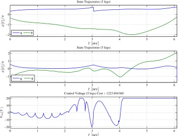
will be presented. The rimless wheel studied in this work has n ₌5 legs

and the angle between legs is α₌ _n2π. Also it was assumed for the sim-ulations that the motor was attached to a fixed frame. This implies that

˙ ψ₌θ.˙

4.4.1 Single Colliding Step

This was the first experiment. The motivation was to determine a set of

initial and final conditions that will provide us with a successful dynamic

step. Table1summarizes the state bounds used in the numerical solution of this experiment.

The first two rows show the constraints on the initial conditions x(to). As

(52)

Table 4.3: Experiment 1 State Constraints State φ(t) φ˙(t) θ(t) θ˙(t)

Minimum Initial π−α

2 0 −2π −3π Maximum Initial π−α

2 π 2π 3π Minimum Bound π−α

2 −2π −2π −3π Maximum Bound π+α

2 4π 2π 3π Minimum Final State π+α

2 −2π −2π −3π

Maximum Final State π+α

2 4π 2π 3π

This indicates to the numerical solver thatφ(t0) is fixed. Another

impor-tant constraint is ˙φ(t0). Since we are only interested in forward steps ˙φ(t0)

is constrained to be non-negative. The other constraints on the

remain-ing initial condition are given to prevent the system from deviatremain-ing from

physically safe values.

The third and fourth rows of Table 1 show state trajectory bounds. Any state trajectory produced by the solver must remain between these

val-ues. The bounds forφ(t) were selected to allow free motion in a forward

step. Each of the other state bounds were selected to keep the system in a

physically meaningful state.

Constraints on the final state x(to) are imposed only on the angle φ(tf)

which defines when a step is completed.

In addition to the above state bounds it is also necessary to specify bounds

on the control input and the final time. Recall that if the final time is fixed

(53)

timetf was free .

Variable V tf

Minimum ₋20 0.1

Maximum ₊20 100

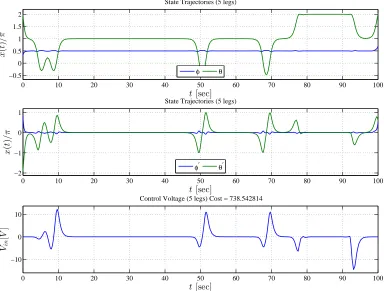
One of the factors that affects more dramatically the trajectories of the

rimless wheel is the choice of cost function. The cost function initially

used to generate an optimal trajectory was the integral of the square of

the input voltage (4.3).

J(tf)= Z t_f

to

V(t)2d t (4.3)

Once the cost function was selected, the optimal control problem is

com-pletely defined. The dynamic equations, system bounds, initialization

in-formation, and cost function were encoded in the files requires by

GPOPS-II and after setting additional information about the nonlinear solvers the

optimization problem was executed.

As shown in Figure4.1, we can see that a colliding step was achieved, but the step required significant amount of time. Furthermore the control

action attempted to stabilize the wheel at its unstable equilibrium before

completing the step. This is definitely not an efficient locomotion gait.

The lesson learned from this simple experiment is that the choice of cost

function plays a very important role in the generation of practical

(54)

0 10 20 30 40 50 60 70 80 90 100 −0.5 0 0.5 1 1.5 2 t[sec] x ( t ) / π

State Trajectories (5 legs)

0 10 20 30 40 50 60 70 80 90 100

−2 −1 0 1 t[sec] x ( t ) / π

0 10 20 30 40 50 60 70 80 90 100

−10 0 10

Control Voltage (5 legs) Cost = 738.542814

Vin [ V ] t[sec] φ θ

[image:54.612.119.503.95.386.2]

φ′ θ′

Figure 4.1: Single Colliding Step with Voltage Cost

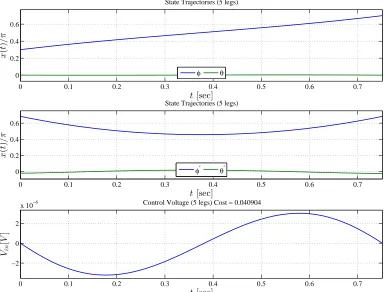
To achieve a better “coordination” a cost penalizing all the states was

used. A revised cost function was created as seen in equation (4.4). This cost function penalized the φ, ˙φ and θ 10000 times less than the input

voltage, and ˙θ1000 times less than the input voltage.

J ₌

Z t_f

to

µ 1

100φ(t)

2

+₁₀₀1 θ(t)2₊ 1 100φ(˙ t)

2

+₁₀1 θ(˙ t)2₊100V(t)2

¶

d t (4.4)

The resulting trajectory is shown in Figure 4.2. Note that now the input voltage is essentially zero (on the order of 10−6_{) and the step is swift.}

The above cost function penalizes excessively the control action and as a

(55)

0 0.1 0.2 0.3 0.4 0.5 0.6 0.7 0

0.2 0.4 0.6

t[sec]

x

(

t

)

/

π

φ θ

0 0.1 0.2 0.3 0.4 0.5 0.6 0.7

0 0.2 0.4 0.6

t[sec]

x

(

t

)

/

π

φ′ θ′

0 0.1 0.2 0.3 0.4 0.5 0.6 0.7

−2 0 2

x 10−6 Control Voltage (5 legs) Cost = 0.040904

Vin

[

V

]

[image:55.612.118.502.95.387.2]

t[sec]

Figure 4.2: Single Colliding Step with a Multi State Cost

The optimal solution provides the initial conditions that give the wheel

just enough velocity for the wheel to lift–off and keeps the internal

pen-dulum close to its stable equilibrium since that does not require much

input voltage.

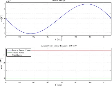
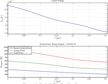
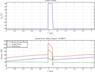
An energy analysis of this input trajectory can be seen in Figure 4.3. In this graph the power output of the motor on the system is plotted. To

de-termine whether the control signal was efficient, the integral of the power

output is calculated. This is done by bypassing the motor and

determin-ing the power of the torque on the system, as produced by the motor. This

(56)

0 0.1 0.2 0.3 0.4 0.5 0.6 0.7 −3

−2 −1 0 1 2 3

x 10−6 Control Voltage

Vi

n

[

V

]

t_[sec]

0 0.1 0.2 0.3 0.4 0.5 0.6 0.7

0 5 10 15

t_[sec]

P

ow

er

[W

]

System Power. Energy Integral = 0.001559

[image:56.612.117.503.96.394.2]

Passive System Power Torque Power Total Power

Figure 4.3: Single Colliding Step Energy

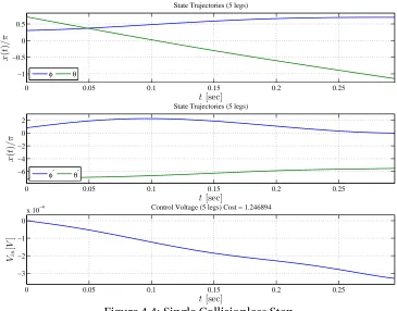
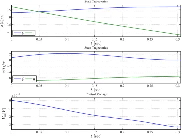
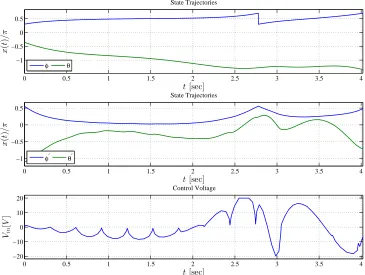
4.4.2 Single Collisionless Step

The second experiment performed focused on creating a collisionless step.

This is a step where the wheel impacts the ground at zero velocity, e.g.,

φ(tf)=0. The goal of this experiment was to determine the type of

mo-tion, initial conditions, and terminal conditions that would be required

to create this collisionless scenario.

The bound for this experiment are given in Table 4.4. As can be seen in the table, φ(t0) is fixed and ˙�

Dynamic Optimization of a Rimless Wheel with an Actuated Pendulum

Dynamic Optimization of a Rimless Wheel with an

Wheel with an Actuated Pendulum

Abstract

Dynamic Optimization of a Rimless Wheel with an Actuated Pendulum

Contents

Abstract . . . ii

5 Conclusions . . . 86

List of Figures

List of Tables

Chapter 1

Chapter 2

Chapter 3

3.1 Newton-Euler Equations

3.2 Lagrangian Dynamics

3.3 Actuator Dynamics

3.4 Collision Dynamics

3.5 Overview of Optimal Control Theory

Chapter 4

4.1 Overview of Implementation

rimlessWheelEndpoint.m

rimlessWheelContinuous.m

rimlessWheelEndpoint.m

4.3 Program Setup

4.4 Experiments

4.4.1 Single Colliding Step

4.4.2 Single Collisionless Step