Finite lattice methods in statistical mechanics

F inite L attice M ethods

in

S tatistical M echanics

Murray T. Batchelor

A thesis submitted fo r the degree o f Doctor o f Philosophy o f the Australian National University

ABSTRACT

This thesis is concerned with the finite lattice study of spin models. The underlying theme in Parts I and II is the exploitation of Bethe ansatz equations to provide finite lattice data well beyond the range normally available.

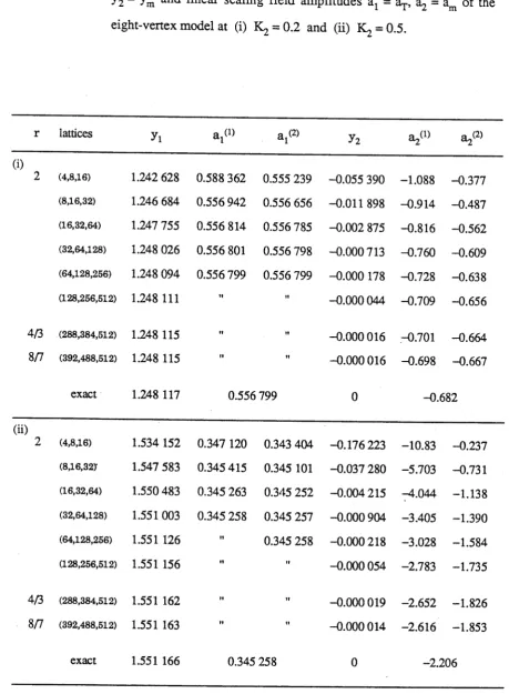
In Part I the Bethe ansatz equations for eigenvalues of the eight-vertex model are solved numerically to yield mass gap data on infinitely long strips of up to 512 sites in width. The finite-size corrections, at criticality, to the free energy per site and polarization gap are found to agree with recent studies of the XXZ spin chain. The leading corrections to the finite-size scaling estimates of the critical line and thermal exponent are also found, providing an explanation of the poor convergence seen in earlier studies. Away from criticality, the linear scaling fields are derived exactly in the full parameter space of the spin system, allowing a thorough test of a recently proposed method of extracting linear scaling fields and related exponents from finite lattice data.

In Part II, the numerical solutions of the Bethe ansatz equations for the eigen-energies of the XXZ Hamiltonian on very large chains are used to identify, via conformal invariance, the scaling dimensions of various two-dimensional models. With periodic boundary conditions, eight-vertex and Gaussian model operators are found. The scaling dimensions of the Ashkm-Teller and Potts models are obtained by the exact relating of eigenstates of their quantum Hamiltonians to those of the XXZ chain with modified boundary conditions. Eigenstates of the Ashkin-Teller and Potts models with free boundaries are also obtained, allowing an examination of their critical surface properties.

ACKNOW LEDGEM ENTS

I wish to record my gratitude and sincere thanks to my supervisor, Professor M. N. Barber, ffom whom I have learnt a great deal over the years; Michael's vitality and enthusiasm alone can inspire those around him. I am also grateful to Francisco Alcaraz, Rodney Baxter, Chris Hamer, Jaan Oitmaa, Paul Pearce and Reinhout Quispel. I have been fortunate to know and work with all of these people. I also thank Brian Davies for friendly advice.

The members of the Mathematics Department have offered cheery support, especially Tina and Clare. Chris Lenard and Yousong Luo have been my fellow students. Thanks are also due to the members of the Colloid and Surface Science group, who have always made me welcome in their department and at their social gatherings. My contemporaries in that group, Phil Attard and Stan Miklavic, continue to be my good friends.

Neville Smythe and Geoff Huston have proven to be extremely helpful system gurus on, respectively, the Macintosh and the Vaxcluster. Anna Zalucki has helpfully typed parts of this thesis as MSR reports.

Throughout the research embodied in this thesis I have been supported by a Commonwealth Postgraduate Research Award, and, while at the University of NSW, a Gordon Godfrey Scholarship.

PUBLICATIONS

1. Bethe ansatz calculations fo r the eight-vertex model on a finite strip M. T. Batchelor, M. N. Barber and P. A. Pearce,

Submitted to J. Stat. Phys.

2. Conformal invariance and the spectrum o f the X X Z chain F. C. Alcaraz, M. N. Barber and M. T. Batchelor,

Phys. Rev. L ett.58, 771-774 (1987).

3. Conformal invariance, the X X Z chain and the operator content o f two-dimensional critical systems

F. C. Alcaraz, M. N. Barber and M. T. Batchelor, In preparation.

4. The surface exponents o f the quantum XXZ, Ashkin-Teller and Potts models F. C. Alcaraz, M. N. Barber, M. T. Batchelor,

R. J. Baxter and G. R. W. Quispel,

Report # 7, Mathematical Sciences Research Centre, ANU (1987). Submitted to J. Phys. A

5. Conformal anomaly and surface energy fo r Potts and Ashkin-Teller quantum chains

C. J. Hamer, G. R. W. Quispel and M. T. Batchelor,

Report # 9, Mathematical Sciences Research Centre, ANU (1987). Submitted to J. Phys. A

6. Critical behaviour o f the BN N N I model in two dimensions J. Oitmaa, M. J. Velgakis, M. T. Batchelor and M. N. Barber, J. Magn. M agn. Mater. 54-57, 665-666 (1986).

7. A finite lattice study o f the critical behaviour o f the two-dimensional biaxial next-nearest-neighbour Ising model

J. Oitmaa, M. T. Batchelor and M. N. Barber, J. Phys. A. 20, 1507-1519 (1987).

8. Sparse matrix factorizations o f transfer matrices M. T. Batchelor,

TABLE OF CONTENTS

Chapter 1 Introduction

1.1 The finite lattice method 1

1.2 Structure of the transfer matrix 4

PART I

Chapter 2 Bethe ctnsatz calculations for the eight-vertex model on a finite strip

2.1 Introduction 10

2.2 The Bethe ansatz equations for the eight-vertex model 12

2.3 Finite-size scaling 26

2.4 Linear scaling fields 39

2.5 Summary and conclusion 43

Appendices 45

PART n

Chapter 3 Conformal invariance, the XXZ chain and the operator content of two-dimensional critical systems

3.1 Introduction 55

3.2 The Bethe ansatz and the spectrum of the XXZ chain 58

3.3 Operator content of the periodic XXZ chain 76

3.4 The XXZ chain and the critical behaviour of the

Ashkin-Teller model 89

3.5 The XXZ chain and the critical behaviour of the Potts models 102

Chapter 4 _{Surface exponents and surface energy of Potts and} Ashkin-Teller quantum chains

4.1 Introduction ₁₁₇

4.2 Bethe ansatz ₁₁₉

4.3 Conformal anomaly and surface energy ₁₂₅

4.4 Surface exponents ₁₂₇

4.5 Exact surface free energy ₁₃₀

PART

m

Chapter 5 A finite lattice study of the critical behaviour of the two-dimensional

5.1

biaxial next-nearest-neighbour Ising model

Introduction ₁₃₁

5.2 Block diagonalization of the transfer matrix ₁₃₄

5.3 Sparse factorization of the transfer matrix ₁₃₅

5.4 Nature of the leading eigenvalues ₁₄₄

5.5 The finite lattice method ₁₄₅

5.6 The ferromagnetic region ₁₄₇

5.7 The anti-phase region ₁₅₀

5.8 Conclusion ₁₅₂

Appendices ₁₅₃

1

INTRODUCTION

1

The idea of a transfer matrix, first introduced by Kramers and Wannier (1941), has gready facilitated the growth in knowledge of statistical systems. Indeed, with hindsight, we can appreciate that Onsager’s original and masterly contribution to the exact solution of the two-dimensional Ising model (Onsager 1944), by explicitly diagonalizing the transfer matrix, heralded in a whole new era in the study of phase transitions and critical phenomena. In subsequent years, a number of models have appeared bearing the title "exactly solved". Perhaps the most famous of these is the eight-vertex model solved by Baxter (1972). This model, in magnetic spin language, contains Onsager's model as a special case when the novel four-spin interactions are absent.

However, many models of physical interest are sufficiently complicated so as to give the impression that they will never be solved exactly. For such models, arguably the most powerful numerical method in two dimensions is the application of phenomenological renormalization to finite lattices.

1.1 THE FINITE LATTICE METHOD

Phenomenological renormalization, introduced by Nightingale (1976, 1979), is a consequence of finite-size scaling (Fisher 1971; Fisher and Barber 1972). Recent reviews of this technique have been given by Barber (1983a) and Nightingale (1982). To illustrate the ideas, we consider here a simple one parameter system* defined on an

*

2

infinitely long strip o f width L in two-dimensions. Let \|/(t) be some quantity which in the infinite system diverges at the critical temperature tc:

\|/(t) ~ A I At I“ 05 as At = t - t c -> 0 . (1.1.1) Here, this critical singularity is "rounded o ff' due to the system's quasi-one-dimensional nature (see B arber 1983a). Finite-size scaling asserts that in the finite system, the behaviour o f \|/( t; L) is described by

; L) - L“" Q^L/SCt)] , (1.1.2)

where £(t) is the correlation length o f the infinite system, diverging as

^(t) ~ I At I , A t —» 0 . (1.1.3)

In (1.1.2), to recover the behaviour (1.1.1) in the limit L -> °o at fixed (small) At we require the scaling function, Qv(z), to satisfy

Q¥(z) - z"“* as z —> . (1.1.4)

In particular, if we choose the quantity \|/(t) to be the correlation length itself, then its behaviour in a finite system can be described by the ansatz

£ ( t ; L ) - L Q ^ [L 1/VA t] , L - > ~ , A t 0 , (1.1.5) which follows from (1.1.2) (here, for convenience, we have m odified the argument of the scaling function). From this result, tc can be estim ated from the sequences of values o f t for which successive ratios o f £ ( t ; L) and ^ ( t ; L') exactly scale, i.e. the values o f t for which

$ ( t ; L ) /L = Z,(t; L ') / L '. On the other hand, by differentiating (1.1.5), we observe that

9 5 ( t ; L)

at _{t= tc} L 1+1/v

(1.1.6)

(1.1.7)

(1.1.8)

J2n (L/L')

The result (1.1.6) is equivalent to Nightingale's phenomenological renormalization criterion (see Barber 1983a). By regarding this equation as a renormalization in the temperature variable the result in (1.1.8) can be obtained in the usual renormalization group manner (see, e.g. Barber 1977, 1983a). In practice, the correlation lengths £(t ; L) appearing in these results are related to the ratio of eigenvalues of the system's transfer matrix. For a simple Ising model this matrix is of size 2L x 2l . From a computational point of view, the largest matrix that can be handled for many models is that for a strip of width L = 16. Nevertheless, the finite lattice method has proven to be extremely powerful (particularly here in two dimensions) and has provided valuable information on the phase diagrams and critical exponents of many models of physical interest. Of course, the underlying spirit of the method is to use strips of the greatest possible width from which one can more confidently infer the phase boundaries and critical exponents of the system under consideration.

The models appearing under the "exactly solved" banner naturally provide excellent testing grounds for any numerical technique. One of the early achievements of the finite lattice method was Nightingale's success in reproducing the critical behaviour of the eight-vertex model in its spin formulation (Nightingale 1977, 1979). There the eigenvalue data was restricted to strips of up to L = 16 and despite this success, poor convergence of the conventional finite-size estimates was seen when the four-spin coupling became large in magnitude. This was also apparent in a subsequent study made by Barber (1985). From a historical point of view, the major goal of this thesis was to extend the available finite lattice data for the eight-vertex model, with the prime motivation being to explore the convergence, with increasing system size, of various aspects of the finite lattice method.

(Baxter 1972, 1973a). The first approach consisted of finding a parametrization of the vertex weights admitting the construction of commuting transfer matrices. On an equal, though more elaborate, footing is Baxter’s generalization of the Bethe ansatz (Bethe 1931). Each technique resulted in a set of functional equations implicitly defining all eigenvalues of the transfer matrix from which the passage to the thermodynamic limit could be made. However, no use has been made of the resulting "generalized" Bethe ansatz equations on a finite lattice; an added motivation for this work was thus the solution of the equations themselves.

The results of this study are presented in Part I of the thesis. Apart from early consultation with Paul Pearce, who helped me to understand and develop a feeling for elliptic functions (and in particular, the conjugate modulus form of the vertex weights and functional equations), the bulk of the work in that part is my own. In particular, I have independently developed the methods and programs to solve the Bethe ansatz equations. Similarly, the finite-size solutions of the "ordinary" Bethe ansatz equations (namely those associated with a six-vertex model or XXZ spin chain) presented in Part II, are my own. These results have played a fundamental role in the formulation of our results. However, before proceeding to these results, we briefly review some of the profound developments that have recently taken place in the theory of critical phenomena. (Reviews of these developments have been given by Fisher 1985, 1986, Friedan et al. 1986 and Cardy 1986c, 1987.)

1.2 STRUCTURE OF THE TRANSFER MATRIX

(1.2.1)

-2h -2h

((^ a ( z l > Z i ) O a ( Z2 , Z2 )) = (Zj — Z2 ) (Z-^ — Z2 ) ,

where (ha, ha) are (real) anomalous dimensions associated with the operator O . Under the conformal mapping w = / ( z), the correlation functions for a conformally invariant system transform as

(Oa^zl » zl ^ a ^ z2 , z 2^

In particular, Cardy (1984a) has chosen m = ^ f i n z ,

dw : dw 2

h_a

dw 1 d w 2

dz1 dz2 _{d z1 d z2} (Oa(W]L, Wl )Oa(w2 , W 2 ) ) .

(1.2.2)

(1.2.3) which maps the full z-plane onto periodically repeated strips of width L. With this choice, the correlation function in the strip, through (1.2.1) and (1.2.2), is

2(h+h )

( ° a ( W l > w l ) O a ( w2 , W o)}

2jt L

7t

2 sin h — (w1 - w 2) 2 sin h “ (wj - w2)71

(1.2.4) Setting Wj - uT + ivl and w2 = u2 + iv2, this has the expansion, for ux > u2,

L j . 2 aj ai exp

J J , J = 0

- J J - (x+j+j'X Uj-U g) exp ( s + j - j ’XVj-Vg)

where

r(x + j)

(1.2.5)

(1.2.6) J H x) j!

The correlation length in the strip can alternatively be evaluated using the transfer matrix. Writing the transfer matrix operator as T = exp(—aH), where a is the lattice spacing, we have (again for ut > i^),

(Oa(u1, v1)Oa(u2>v 2)) =

V , I A ■ -(E - E0)(u,- a,) A

2 , < ° | O a( v i ) |n ,k > e < n ,k |O a(v2) |0 ) , (1.2.7)

n

where I n , k ) is a complete set of eigenstates of H with energy En and momentum k (quantized in units of 27t/L). Comparing this result with (1.2.5), we see that for each primary operator Oa of dimension xa and spin sa there exists an infinite tower of

A

eigenstates of H, labelled by j and j ’, with energy E0 + 27t(xa + j + j')/L and momentum 27i(sa+ j - j ’)/L.

We see that the location and ordering of the levels in the finite lattice eigen-spectrum is thus determined by the anomalous dimensions of the operator algebra describing the critical behaviour of the infinite system. The same structure is found in the eigen-spectrum of critical quantum Hamiltonians (von Gehlen et al. 1986). At the heart of this discovery is Cardy’s exploitation of conformal invariance. That conformal invariance should be exhibited by correlation functions at a critical point was first suggested by Polyakov (1970). Basically, for conformal invariance to hold, the system is assumed to possess scale invariance (in the renormalization group sense) and both translational and rotational invariance as well as short range interactions. Cardy's results explained the previously observed connection between finite-size scaling amplitudes in strips and critical exponents and have since been verified in a number of models (see, e.g. the review by Cardy 1987 and Section 3.1, following).

characterized by a particular number, the so-called "central charge" or "conformal anomaly . Friedan, Qiu and Shenker (1984) showed that for unitary models with conformal anomaly number, c , less than unity, c must be quantized according to

c 1 - 6

m{m + 1) for m = 3 , 4 , . . . , (1.2.8)

and that the allowed values of the scaling dimensions of the primary operators (i.e. those forming the "starting points" of Cardy's towers) are (h , h—) where_{pq pq'}

[ p ( m + l ) - q m ] - 1

hw = --- Tm jrn + 1)--- ’ (1-2-9>

with l < q < p < m - l . This is the Kac formula (Kac 1979). (This result has helped to explain why so many critical exponents in two dimensions are rational numbers.) For given m (and thus c), various models, in different universality classes, have been identified in this scheme (see, e.g. Cardy 1987). Blöte, Nightingale and Cardy (1986) and Affleck (1986) have shown that c is directly related to the leading finite-size correction to the free energy per site of the infinitely long strip. This result gives a way of "measuring" c for a given model (though, as we shall see in Section 3.3.4, care has to be taken in some cases).

In analyzing the eight-vertex model Bethe ansatz equations, I naturally looked at the numerical solution of the simpler equations of the XXZ chain. The motivation for this was associated with the question of completeness. In principle, the Bethe ansatz equations give all of the eigenvalues, but how many could we compute by actually solving the equations? It turns out that several distributions of zeros are particularly simple and the corresponding eigenvalues can be computed on relatively large chains. However, in the course of this work, we became aware of Cardy's results and had some very nice slices o f luck. I would like to record some of these developments here as a prologue to Part II of the thesis.

8

coupling A = 0. To our surprise, it agreed, apart from a normalization factor and a doubling of lattice size, with Francisco's ground-state formula at the decoupling point of the critical Ashkin-Teller Hamiltonian (Kohmoto et al. 1981). Was this just coincidence? Numerically, we tried some other couplings. To outelation, the two ground-states were

exactly related on finite chains for all values of the couplings. We looked at other energies in the eigen-spectra and found common levels in the two models. This was a real breakthrough; since the early calculations of Alcaraz and Drugowich de Felicio (1984), eigenvalues of the Ashkin-Teller model have only been calculated on chains of up to length L = 10. By numerically solving the Bethe ansatz equations for the corresponding levels in the XXZ Hamiltonian we could then obtain levels in the Ashkin-Teller model for chains of length up to L = 256 with relative ease.

Here we began to draw on Michael Barber's experience. Besides conformal invariance, there is a further idea unifying the theory of critical phenomena in two dimensions. This is the notion that there exist general models to which specific models of physical interest can be related by appropriate transformations (see, e.g. Nienhuis 1984 and references cited therein, Kadanoff and Brown 1979, Knops 1980, den Nijs 1981). Examples of such "central theories" are the Coulomb (lattice) gas (Nienhuis 1984) and the generalized Gaussian model (Kadanoff and Brown 1979). Analysis of these models can yield detailed information on the critical behaviour of the related physical models. We shall see in Chapter 3 that the anomalous dimensions appearing in the XXZ model are directly related to those found in the Gaussian model.

A natural question that arose was: "Can we also locate energy levels of the critical Potts models in the eigen-spectrum of the XXZ Hamiltonian?" Indeed, it turns out that we can, though the XXZ Hamiltonian needs a special "twisted" boundary condition for which I have derived Bethe ansatz equations and have again solved numerically. Like the Ashkin-Teller model, eigenvalues of the Potts Hamiltonian (Solyom and Pfeuty

1981) had only previously been calculated on small chains.

was largely carried out by Francisco Alcaraz and Michael Barber.

Cardy's argument is also applicable to systems with free boundary conditions along the edges of the strip (Cardy 1984a). Antiperiodic (or "twisted") boundary conditions can also be encompassed (Cardy 1984b, 1986b). Thus we have also examined the predictions of conformal invariance for the Ashkin-Teller and Potts models with free boundaries. This work is presented in Chapter 4. In this case the Bethe ansatz solution of the XXZ Hamiltonian with free edges had been previously derived by Gaudin (1971, 1983). However, the Hamiltonian corresponding to the free edge Potts model was "unsolved" and the equations were largely derived for us by Rodney Baxter. Again it turns out that the Bethe ansatz equations can be solved numerically for levels in the "equivalent" XXZ Hamiltonians to provide eigenvalues in the spectra of the critical Potts and Ashkin-Teller Hamiltonians on relatively large chains, here of length up to L = 256.

Finally, in Part III we present a "conventional" finite-size study of a two dimensional Ising model with competing interactions between first- and third- nearest-neighbour spins. Such models are capable of exhibiting rich and complex critical behaviour, particularly when the competition is between antiferromagnetic and ferromagnetic interactions. For this model, the nature of the transition when the antiferromagnetic third-nearest-neighbour interactions were sufficiently strong was unclear; we hoped to settle the issue by using the finite lattice method. This work complements the series analysis of Oitmaa and Vegakis (1987) and was suggested by Jaan Oitmaa.

Independently, I have developed a "graphical" method to help write down the sparse factors of a given transfer matrix. Such factorizations highlight the internal structure of the matrix. This can be exploited in the numerical computation of the leading eigenvalues. However, as we have seen above and shall see in the following, there is further structure to be found in the levels of the eigen-spectrum at criticality, with the

10

BETHE ANSATZ CALCULATIONS FOR

THE EIGHT-VERTEX MODEL ON A

FINITE STRIP

2

2.1 INTRODUCTION

The exact solution of many integrable models in statistical mechanics and field theory, in one form or another, involves the Bethe ansatz and its generalizations (see, e.g. Lieb and Wu 1972, Thacker 1981, Fowler 1982, Baxter 1982, Gaudin 1983 and Tsvelick and Weigmann 1983). Generally, the Bethe ansatz equations constitute a set of transcendental equations whose solutions characterize a given eigenvalue and corresponding eigenvector of the transfer matrix or quantum Hamiltonian of the model. In the thermodynamic limit, the number of equations and solutions become infinite, but the equations can be transformed (see, e.g. Lieb and Wu 1972 and Baxter 1982) to linear integral equations, which, at least for the dominant eigenvalues that are required for thermodynamic functions such as the free energy or surface tension, can be solved by the use of Fourier transform techniques.

Despite these successes of the Bethe ansatz in the thermodynamic limit, little use has been made, until recently, of the Bethe ansatz to evaluate quantities on finite lattices. This is somewhat surprising since solution of the Bethe ansatz equations for a finite system could provide considerable information on the behaviour of not only the finite system itself but also of the bulk system. In particular, the critical behaviour of the bulk system could be explored by finite-size scaling techniques (see, e.g. Barber 1983a).

and Woynarovich (1985) originally applied this method to the non-critical region of the XXZ Heisenberg chain. Hamer (1985, 1986a) and Woynarovich and Eckle (1987) have, however, shown how to extend the method to calculate finite-size corrections at criticality, and hence to infer critical exponents of the bulk XXZ system; see also Hamer, Quispel and Batchelor (1987). Similar work has been reported for the XYZ chain (Martin and de Vega 1985) and the eight-vertex model (Hamer 1986b).

The method of de Vega and Woynarovich represents the solution of the Bethe ansatz equations for a large finite system as a perturbation (by a sum of delta functions) of the density function that describes the solutions for the infinite lattice. An alternative approach to exploit the Bethe ansatz for a finite lattice is to directly solve the (finite) set of equations for the (finite) number of solutions characterizing the eigenvalues of the finite lattice theory. This is the approach we adopt here for the eight-vertex model; critical parameters being obtained by finite-size scaling techniques.

Several attempts at direct solution of the Bethe ansatz equations for a finite lattice have been reported for the isotropic Heisenberg chain. In particular, Grieger (1984) and Borysowicz et al. (1985) have computed ground-state correlation functions. Avdeev and Dörfel (1986) have obtained the leading correction to the ground-state energy and explored the way in which the density of solutions approaches the bulk limit solution of the integral equation. Woynarovich and Eckle (1987) have computed the lowest state in the two largest sectors of the critical XXZ chain, complementing their analytic analysis of the dominant finite-size corrections appearing in the model.

In this chapter, we directly solve the Bethe ansatz equations for the eight-vertex model. Our motivation, beyond the solution itself of the equations, is to explore the convergence of finite-size scaling and related techniques for this model. Early finite-size calculations (Nightingale 1977, 1979, Barber 1985) for the eight-vertex model were based on finite lattice data obtained by direct diagonalization of the transfer matrix in the spin formulation. As a result, eigenvalue data was restricted to strips of width up to 16 sites. While the estimates of bulk critical exponents were quite consistent with the exact results, several aspects warrant further investigation with data from larger lattices. Conventional phenomenological renormalization estimates converge well for small values of the four-spin coupling. However, the convergence deteriorates significantly as the magnitude of the four-spin coupling increases and, indeed, appears to become non-monotonic. Data from large strips would clearly allow a non-trivial test of finite-size seating and related techniques for a system with non-universal behaviour.

The arrangement and content of this chapter is as follows. In Section 2.2, we reformulate and examine the Bethe ansatz equations of the eight-vertex model. We then proceed to numerically solve these equations for the two simplest distributions of zeros. In Section 2.3 we define a mass gap from the corresponding eigenvalues and discuss the convergence rates of finite-size estimates of the critical line and thermal exponent. Finally in Section 2.4 we derive exact expressions for the linear scaling fields in the full parameter space of the eight-vertex model. In this section we implement and fully test a recently proposed method (Barber 1983b, 1985) of extracting linear scaling fields from finite lattice data. The chapter closes with a summary of our results.

2.2 THE EIGHT-VERTEX MODEL BETHE ANSATZ EQUATIONS

2.2.1 Parametrization and functional equations

13

the elliptic function

o o

~ . 1 I , m-1 m -1 m

fiz,q) = X

X

( i — q Z^ 1 “ ^ Z X! ~ Q ) (2.2.1a)

m=l

m+1 m(m+l)/2

» q (2.2.1b)

where nome q = e- e , e = tcI'/I with I and I' the complete elliptic integrals of the first kind. The usual elliptic theta functions @(z,q), H(z,q) and h(z,q) = @(z,q)H(z,q) which appear in Baxter's formulation are related to this function by

Some useful properties of the elliptic function (2.2.1) are listed in Appendix 2A.

The connection between the spin and arrow formulations of the model was discovered originally by Wu (1971) and Kadanoff and Wegner (1971); see also Baxter (1982). The allowed arrow configurations, along with one of the two equivalent sets of spin configurations are shown in Figure 2.1. Defining a set of spin couplings K = (Kj, Kj', K^) as in Figure 2.2, the vertex weights are

c = R exp(K 1 - Kj' - K J , d = R e x p (- K x + K / - B y , (2.2.3) where R is a normalization factor. In terms of the elliptic function defined in (2.2.1) these weights can be written

2 1/4 - 1/2 2

©(z,q) = f(qz,q ), H(z,q) = iq z flz,q ) , (2.2.2a)

flq,q3)

(2.2.2b)

a = R exp(K 1 + K j' + K^) , b = R e x p (- K x - K / + Kj),

f(qx 1z,q2) flqxz,q2) flq,q2) flqx2,q2) x 1/2 flqx-1z,q2) flxz,q2)

z 1/2 f(q,q2) f(x2,q2)

^ q1/2 f(x l ZyC?) f(xz,q2) z f(q,q2) f(qx2,q2) x3/2 f(x 1z,q2) f(qxz,q2)

z 1/2 flq,q2) flx2,q2)

, (2.2.4a)

, (2.2.4b)

where

Figure 2.1 _{The standard arrow and spin configurations of the eight-vertex model} and their corresponding weights. An equivalent set of spin configurations has all spins reversed.

[image:21.552.52.506.76.762.2] [image:21.552.83.495.80.326.2]

14

Since we will focus on the transition from the ferromagnetic ground-state we have rearranged the parametrization of the weights compared to Baxter's arrangement (Baxter 1973b). (The interchanges are a c , b <-» d). A sa result the critical line is given by

a = b + c + d (2.2.6)

or

sin h 2Kj sin h 2 K { = exp ( - 4 K ,) . (2.2.7) In the low temperature (ferromagnetic) regime (a > b + c + d) we have

0 < q < x2 < 1 , x < z < x_1 . (2.2.8) The symmetric case Kx = is given by z = 1 , here c = d . The Ising limit 1^ = 0 is given by q = x4, where ab = cd. The parametrization (2.2.4) is such that q = 0 in the low temperature limit and q = 1 at criticality.

All eigenvalues T(z) of the row-to-row transfer matrix (Baxter 1972) are implicitly defined through the functional relation

(_)v +v T(z) Q(z) = P(xz) Q(x 2z) + P(x~‘z) Q(x2z) where

P(z)

x ffz,q)

/ z f(x2,q) N = 2 n ,

Q(z) = z-(n+v)/2

(2.2.9a)

(2.2.9b)

(2.2.9c)

The condition on the n zeros is

1 .

v i -j = i

n

("2 ^ v.) / I = n + v" + even integer ,

which can also be written

j = i

zj =

n+v v/2

q

(2.2.10)

The quantum numbers v’ and v" satisfy the following rules : v = 0(1) if the number of down arrows in a row is even(odd)

v" = 0(1) if the corresponding eigenvector is symmetric(antisymmetric) with respect to arrow reversal.

A further quantum number v is defined via the condition

v + v' + n = even integer , (2.2.12)

implying that we can choose v = v' for n even, and for n odd; v and v' to differ by one. For convenience, in all subsequent numerical computations we take n to be even, and thus N to be a multiple of four.

The generalized Bethe ansatz equations provide the zeros of the function Q(z). These equations are obtained by setting z = Zj, j = 1,..., n in equation (2.2.9a); the left hand side vanishes, resulting in a set of n coupled nonlinear equations;

2 z i n fix j - ,q)

-2v

TT

k

= - x 1 1 ---2--- > j = 1 ... n - (2.2.13) k » l ry —2 j \

fix

v~

’T)

Zk

fix Zj ,q) flx_1Zj ,q)

The logarithmic form of the eight-vertex equations has been discussed by Johnson, Krinsky and Mc Coy (1973) (see also Takhtadzhan and Faddeev 1979). In our notation we may write the equations as

n

N ® i(fp = -2jrfj - 2 v f in x + X ° 2 (‘t'j " V . j = l , . . . , n . (2.2.14)

Here we have further defined Zj — exp i(j)j . In (2.2.14) the Zj are half-integers and

° p (<W = (p(0»xP) (2.2.15)

where

00' m

cp(<}),x) = 7Ü <(> 2^T —

-m=l

-m m

q ) sin m(|) m ( l - qm)

(2.2.16)

2.2.2 Solution on a finite lattice

Equations (2.2.13) and (2.2.14) have not been solved for general values of q, x, and n. In this chapter we are only interested in their solution as a means of providing the two largest eigenvalues from which we define a suitable mass gap. For even n, the maximum eigenvalue T0(z) has v = 0 while the next largest, T^(z), has v" = 1. Both eigenvalues are in the sector with v' = v = 0.

Bootstrapping in temperature

The first order approximation (q « x2 « 1) has been carried out by Baxter (1972). In this limit (2.2.13) reduces to

n v"

Zj + (-) = 0 , j = 1,..., n (2.2.17) z.e. the zeros characterizing T0(z) and Tx(z) are the interlacing nth roots of ± unity. The corresponding limit in (2.2.14) indicates the following choice for the numbers Zj:

T0(z): Zj = j - 1 / 2 , j = l , . . . , n (2.2.18a) Tt (z): Z j = j + l / 2 , j a l ... n (2.2.18b) The distribution of zeros in the complex z-plane for each eigenvalue is shown in Figures 2.3(a) and 2.3(c) for N = 32. These zeros can be used as initial starting points in the numerical solution for either (2.2.13) or (2.2.14). Given a value of x(ti), the zeros are obtained by incrementing q and solving the thus modified set of equations for the new distribution of zeros. This distribution is used as input for another increment in q and so on ... . In this way we "bootstrap” the zeros through their finite temperature distributions. The zeros for T0(z) and Tj(z) at q = 0.1 with q = x3 (tj = iI'/3) are

shown in Figures 2.3(b) and 2.3(d). We observe that the sets of zeros remain interlaced.

Eigurc 2.3 Distributions of zeros on the unit circle in the complex z-plane for eigenvalues T0(z) and T^z) on a strip of width N = 32.

(a) and (c): distributions at q = 0.

lattice sizes N = 4 and N = 8, the eigenvalues obtained in this way with the results of a brute-force" diagonalization of the transfer matrix. In practice, as the zeros Zj occur in complex conjugate pairs, the number of zeros and equations can be reduced to n/2 for T0(z), and n/2 - 1 for Tx(z) where we further factor out the stationary zeros at = 0 and <j>n = k.

Exact solutions in the Ising limit

As an alternative to bootstrapping from the low temperature limit, for a given value of q, the incremention can be in the variable x away from the exact Ising solutions. When q = x^, the Bethe ansatz equations decouple and the solutions can be written in closed form. The simplest approach is via (2.2.14), which reduces to

n

N^OtO = -2nZ. - n ( j t + <t>j) + , j = l , . . . , n . (2.2.19) k=l

On rearranging, this can be written

4>k = am(I(J)j/7t, k ) , _(2.2.20)

where am(u,k) is the elliptic amplitude function of argument u and modulus k (see, e.g. Gradshteyn and Ryzhik 1980) satisfying

u = y (a m (u ,k ),k ) (2.2.21)

where ^ ( 0 ,k ) is the elliptic integral of the first kind:

0

y ( 9 ’k ) = J

f—

d ' f

•

(

2

.

2

.

22

)

o ^11 - k sin a

In (2.2.20) nome q — x. From (2.2.20) and (2.2.21) we have the following results,

T0(z) : <|»j - Ti I 1 y | N Ij2 . k I , j = 1 ,..., n , _(2.2.23a)

_ 27t J K K

Tx(z): <>j - it Iy N lj2 vr > k , j = 1 ,..., n ._(2.2.23b)

18

f

k 271

I

m(m -1) X

2

\ m = 1

(2.2.24)

(2.2.25)

Initial approximation of zeros

For the largest eigenvalue, an initial approximation to the zeros for any values of q and x, increasing in accuracy with system size, can be obtained by generalizing the method outlined by Grieger (1984) in the computation of the ground-state of the isotropic XXZ antiferromagnet. Here we appropriately sample the known (Johnson et al. 1973 and Takhtadzhan and Faddeev 1979) distribution of zeros for T0(z) to provide approximations to the zeros of both leading eigenvalues. To derive the necessary result, we follow Hamer (1986b) and introduce the quantity

ZN((J» - _(2.2.26)

so that, from (2.2.14), at the zeros <}>j we have

= / . / N . _(2.2.27)

Also define

dZj^((j)) d(j>

then (Johnson et al. 1973 and Takhtadzhan and Faddeev 1979) oo

R J * ) = —

X

exp(im(t))

coshmÄ. dn(I<{)/7t,k)

(2.2.28)

(2.2.29)

where dn(u,k) is a standard elliptic function (Gradshteyn and Ryzhik 1980). In (2.2.29), modulus k is defined by

I /I = V7C = - n y i (2.2.30)

(2.2.31) ZJO ) = — am[ I 0/1 f ~~ tu , k~

Finally from Eqs. (2.2.21), (2.2.27) and (2.2.31),

(2.2.32)

should be a good approximation to the zeros <j>j , becoming exact as N —» o o . Realize

however, that (2.2.32) is the result (2.2.23a) obtained in the Ising case. Both of the Ising results (2.2.23a) and (2.2.23b) are thus excellent approximation formulas for all values of q and x. In Table 2.1 the values obtained from these formulae for q = x3 = 0.1 and N = 32 are compared with the exact, numerical, results. As can be seen, the agreement is close, resulting in rapid convergence to the exact zeros.

2.2.3 Comparison with bulk results

For the symmetric case (z = 1) (2.2.9a) simplifies to give the largest eigenvalue in the form

Tn(l) = 2

flx,q) fix ,q)

Y j flx2z q)

(2.2.33)

where we have exploited the fact that the zeros occur in unimodular complex conjugate pairs. However, for v" = 1, (2.2.9a) reduces to the identity "zero = zero". An expression for T j(l) can be obtained by differentiating (2.2.9a) with respect to z and then setting z = 1 (this was a suggestion of Michael Barber). The result is

^ (1) =

-flx,q) nN flx2,q)

g x 2,q) ^ f V fCx2Zj,q)

g d .q ) (2.2.34a)

in which

F(x,q)

£

g(x 2Zj \q ) g(x2z. \ q )

[image:29.552.72.450.86.515.2]

Table 2.1 Approximate and exact (numerical) zeros <j)j characterizing the eigenvalues T0(z) and T L(z) on a strip of width N = 32 for T| = iI73 (q = x3) and q = 0.1.

T0(*> TjCz)

approx. exact approx. exact

0.048 047 0.048 023 0.096 562 0.096 609

0.146 037 0.145 959 0.197 011 0.197 114

0.250 106 0.249 957 0.306 071 0.306 257

0.365 844 0.365 583 0.430 653 0.430 980

0.502 181 0.501 708 0.582 855 0.583 482

0.676 405 0.675 428 0.789 042 0.790 538

0.932 371 0.929 549 1.132 394 1.139 276

20

(2.2.34b) and the function g(z,q) is defined by

(2.2.35)

In Eqn. (2.2.34) we are to agree that z : = 1. There are no such cancellation problems in the nonsymmetric case.

Given T0(z) and T^z), the free energy per site fN and the interfacial tension oN can be defined on a strip of width N as (see, eg. Baxter 1982)

The exact results derived by Baxter (1972, 1973b, 1982), valid in the thermodynamic limit, are

In Table 2.2 we show the values of (2.2.36) and (2.2.37) for z = 1, q = x3 = 0.1 and q = x6 = 0.01 on finite strips of width N = 2l , l = 2, 3,..., 8. For comparison we show also the bulk limits given in (2.2.38) and (2.2.39). The slow convergence of the interfacial tension is presumably a result of the double logarithm in its definition.

It should be noted that the only real limit imposed on the evaluation of T0(z) and T^z) with increasing system size is in the resolution of zeros as q tends to its critical value (as can be seen from Figures 2.3(b) and 2.3(d), the non-stationary zeros will coalesce at z = 1 in this limit). For this reason, to examine the critical region in detail, we have derived an alternative parametrization of the vertex weights (2.2.4) and the functional equation (2.2.9).

-ß fN = ~ ß n T 0(z) , (2.2.36)

T0(z)

(2.2.37) Tx(z) •

(2.2.38)

/

' \4 l

Table 2.2 Finite lattice estimates (2.2.36) and (2.2.37) of the eight-vertex model free-energy per site and interfacial tension. Also shown is the quantity -ß fN^ = N-1 ßn T ^z) .

N

q = x3 = 0.1

-ß fN<°> -p fN<» _{- ß ° N}

q = x6 = 0.01

-ß fN<°> -ß fN(i) _{- ß ° N}

4 0.335 068 0.274 637 0.3550 0.111 023 -0.005 419 0.1910

8 0.311 680 0.295 782 0.2578 0.088 066 0.059143 0.1830

16 0.305 641 0.301 653 0.1720 0.082 064 0.075 222 0.1383

32 0.304114 0.303143 0.1085 0.080 553 0.079 016 0.0941

64 0.303 732 0.303 507 0.0663 0.080181 0.079 862 0.0608

128 0.303 638 0.303 592 0.0401 0.080 092 0.080 035 0.0385

256 0.303 616 0.303 609 0.0248 0.080 073 0.080 066 0.0245

21

2.2.4 Reformulation at criticality

The limit q —» 1 can be handled by using the conjugate nome identities outlined in Appendix 2B. In terms of the conjugate variables

C = ex p (iw ),

x

= ex p (i|i), p = exp(-27t2/e) (2.2.40)

with w = - i27tv/r and p. = - i27rn/T, the vertex weights (2.2.4) may be written

a

. X

K- ^xC .p) fl^/yx .

p

)

C

« -

x

.

p

) « -

i

,

p

)

x g x x i

,

p

)

R'Wx

>

p

)

C

ft-x.p) R-i.p)

c = p

X flVxC ,p)

g -

V^x ,

p

)

C f(% ,p)f(-i,p)

d = _ p

/X g-^XC , p ) , p )

V 5 f(x ,p )K -i,p )

The normalization factor p is given by

exp —3— (yi2 - y 2)

2 i r 1

In the ferromagnetic regime, the new variables (2.2.40) satisfy I Z I = I X I = 1 , 0 < p < 1 , |w | < | i < 7 t and the square root is taken so that

- f <arg(;1/2) < |- .

The functional equation (2.2.9) transforms to

(-)

v

'+

v

"

t

(0Q(0 = P(xOQ(x'2Q + P(x_1C)Q(x20

with

(2.2.41a)

(2.2.41b)

(2.2.41c)

(2.2.41 d)

(2.2.42)

(2.2.43)

(2.2.44)

(2.2.45a)

P(Q

x f(C.p)

ii

Rx2-P2).

22

q(ö

=-

— » / « n J f .

j-1 V^j

(2.2.45c)

Finally, the condition on the zeros (2.2.10) reads

I ! Cj = (~ )v pV"+n+eV • (2.2.46) j-1

The symmetric case (Kx = K^) is now given by w = 0 and the Ising limit (H = iT/4) by fi = rc/2. Duality is given by the simple interchange p «-» - p, criticality occurring at p = 0. From (2.2.45a) the zeros specifying a given eigenvalue are now solutions of

,p2)

,P2)

ftzHjC^p2)

f(r

2% f t 1. P2)

j = 1 ... n (2.2.47)

where, for n even, we have chosen ev = - n. For the symmetric case, the analogous relations to (2.2.33) and (2.2.34) are

T (1) = 2 o

«X.P2) «x2.p2)

r r ^ V )

j=r

r

C

j

.

p

2)

(2.2.48)

T ( l ) = - «x,p2)

f('/2,p2)

Sx2,p2)

ff

X HX.P4) 1 1 ^ , (2.2.49)

g ( l . p ) j.2 «Cj.P)

in which F(%,p2) is as defined in (2.2.34b), only now with z■, x and q replaced by Cj , x and p2. Here the zeros zl = 1 and = -1 map to the values ^ == 1 and ?2=

23

Zeros for T0(£)

On setting ^ = e x p (-2 0 j) and using the definition (2.2.1) we may write for

example

flxCj >p2) i n sinh(otj -ip/2) 1 + p4m - p2m cosh(2<Xj -ip ) = e ---

[[

---Rr'Cj ,P2) Slnh(ai +i^ 2 ) “ ! + p4m _ p2m COsh(2oCj +in)

(2.2.50) Subsequently on taking logarithms in (2.2.47) we introduce the quantities cp and O

defined by

sin h (a -ip /2 ) exp(itp)

exp(iO )

sinh(a+ip/2)

1 + p2 + 2p cosh(2a - i2p) 1 + p2 - 2p cosh(2a + i2p) with

<p(a,p) = 2 tan kcotp tanha) ,

- l

( \

2p sin h2a sin2p <X>(a,p,p) = 2 tan

1 1 + p^ - 2p cosh2a cos2p For T0(Q the Bethe ansatz equations can then be written in the form

n

NS^otj ,p/2) = 27clj + ^ 'F(aj - a k>p) j = l ,. . . , n

where

k =l

s 2m

¥ (a ,p ) = cp(a,p) + 2 , ) •

m=l

and the Ij are half-integers given by

Ij = (2j - n - l)/2 , j = 1,...,

(2.2.51)

(2.2.52)

(2.2.53)

(2.2.54)

(2.2.55)

(2.2.56)

24

Zeros for T t(£)

The zero C)l = p trivially satisfies the first of the equations (2.2.47). On re-labelling, the remaining n - 1 zeros satisfy

R

x

C

j

.

p

2)

., ««V> f, f

_^X

₂

_{Cg Ck'.P2)}

tfr'Cj.P2)

_{K Kpx_}

₂

_{Cj.p2) k=Aif}

(2.2.58) and subsequently, on taking logarithms,

o o

N'i'Ccij = 2:tlj + X 0 ( 0 ^ , p2m_1)

m=l

n -1

+ 2 h . j = l , . . . , n - l (2.2.59) k = 1

with integers L given by

Ij = j - n + 2 , j = (2.2.60)

Approximation of zeros

Rather than repeating the working in Section 2.2.2 and inverting appropriate elliptic functions, the shortest path to the desired formula is the direct transformation of the final result (2.2.32). Using the identity

I _

i ~ m- r (2.2.61)

(2.2.32) can be used to write

(2.2.62)

2.2.5. _{Bethe ansatz equations and eigenvalues at criticality}

At p 0 the equations (2.2.55), with the choice of the numbers Ij in (2.2.57), reduce to the Bethe ansatz equations describing the leading eigenvalue of either the 6-vertex model or the XXZ chain (Lieb and Wu 1972, Yang and Yang 1966a,b). Correspondingly, the equations (2.2.59) with (2.2.60) describe the leading eigenvalue in the next-largest sector of either model. Defining

ctj = ta n h _1(ta n p /2 tanGj/2), (2 .2.63) the equations for T0© and T ^ Q can thus be written as

r

N9j = 2lcIj - ^ © ( ej.9 k ) > j = l , . . . , r (2.2.64) where

0(0,9') = 2 tan-1 A sin (0 -0 ')/2

(2.2.65) cos(0+0')/2 - A cos(0 -0 ')/2

in which we make the identification A = - c o s p . In (2.2.64), r = n for T0(O and r = n—1 for T /Q .

Finally, in this limit equation (2.2.62) can be evaluated to give the result

(2.2.66)

This last approximation formula wiU be used in Section 3.2.4 for the discussion of the numerical solution of the XXZ Bethe ansatz equations. In this limit the expressions for the two largest eigenvalues, (2.2.48) and (2.2.49), reduce to

Tn(l)

Tj(l)

2 cos(i/2

2 cosp/2

cosh2ctj - cos2p j = i cosf^Oj - 1

1N n /2 -1

n

j = l

cosh2oCj - cos2p.

cosh2cXj - 1

(2.2.67)

(2.2.68)

26

n/2-1

E = 2NcosV 2 - cosn - £ 2 Sm^ Sm24 (2.2.69)

jTi cosh2cx^ - cos2|i

Here we have written the eigenvalues in terms of the zeros on (0,°<>) which we can solve for separately (see also Appendix 2D).

In Figure 2.4 we show the zeros ^ characterizing the eigenvalues T0(Q and Tj(£) at criticality. In the limit p = 1 all of the zeros are at the point £ = 1. As p decreases, apart from the stationary zero at £ = 1, the zeros all move smoothly to the left until at criticality they occupy the positions shown in the figure.

2.3 FINITE-SIZE SCALING

The numerical solution of the eight-vertex model Bethe ansatz equations, described in the preceding section, allows the mass gap

kn = fin(T 0/T1) , (2.3.1)

to be easily evaluated for strips up to N » 256 for general couplings and up to N = 512 at criticality. These values of N far exceed the lattice sizes (N ~ 16) available in previous finite lattice studies of the eight-vertex model (Nightingale 1977, 1979 and Barber 1985). As mentioned in Section 2.1, this allows a non-trivial test of finite-size scaling and a detailed investigation of convergence rates (Privman and Fisher 1983, Barber 1983a). We begin by considering the free energy and mass gap at criticality for which the expected behaviour is predicted by conformal invariance (Cardy 1986a).

2.3.1 Free energy at criticality

For a finite strip with periodic boundary conditions, conformal invariance predicts (Blöte et a i 1986, Affleck 1986) the free energy per site, / N , to approach its

$c-

^

^

^

^

---1 To O

^ ---5fC---^ ^ " H Q

0 1

(2.3.2)

/ n = - L - X N - 2 + o(N ~2) ,

where c is the conformal anomaly (note that we have neglected a factor ß here). For a

model with a line of continuously varying exponents c is expected to be unity (Friedan

et al. 1984). This prediction has been tested by Blöte et al. (1986) using data from strips

o f up to 16 sites. Excellent agreement was found for - 0 .3 < < 0 .4 (0.3 < \\Jti <

0 .7 ) but for outside this range the convergence deteriorated significantly.

From (2.2.36) and (2.2.67) the free energy o f the eight-vertex model on a finite

strip is

-

p

/

n

= ßj

_2cosp/2

_j

ßn2 + ^ ßn j = i

f \

cosh2(Xj -cos2p.

cosh2aj - 1 (2.3.3)

Taking the thermodynamic limit, we have (Lieb and Wu 1972, Baxter 1982)

-ftf.

J cosh2a - cos2p.

2cosp/2j +

J

4ficosh(7toc/|i)

y

cosh2a - 1 (2.3.4a)

The integral appearing in this result also occurs in the exact solution o f the F

model (Lieb and Wu 1972) and has been tabulated by Temperley and Lieb (1971) for

several values o f cos|i. In particular, at ji = 7t/3, k/2 and 2k/3, the exact (Temperley

and Lieb 1971) results are, respectively, ßn2, 2/n x Catalan's constant, and 3/2 J2n(4/3). However, as pointed out by Temperley and Lieb, the integral is awkward

to evaluate numerically because o f the logarithmic singularity at a = 0. In our case, it is

more convenient to use the result (Baxter 1972, 1984).

- ß l P f [cosh(7t-2|i)t - coshjit] [cosh|it - 1] (2 3 4b)

cosp/2

J

+

J

2t sinhTtt coshfit

To estimate c, we define estimators

Cn = f | / ~ " ^n] n 2 . (2.3.5)

which from (2.3.2), should tend to c = 1 as N —» . In Table 2.3 we show the

1 a n o m a ly (c = 1 ) e £ c o CJ <D -G LO <ri CN n_✓ 75 Ü ' S 1 M3 oo <D <D •—■ S • g =1 S-( jy «3

s

§ O , D .G H -O c o "w o c « a a 13 ■8

s

d t: 4J > A G top ’33 <u a <+•4 o m r i a s CC H CM t-H r H 1 LG 1 CM $ © t=i CM S ä 55 © oo

CO s ® _{i o} s_rH

CO LO

rH ©

O CM

© © CM © o CM © CM

O 0 5 O

c o t o c o

CM CO o

CM rH rH*

LO rH

o ©

P ©

rH rH

© © p rH o © © rH l > CO ©

^ LO rH

CO LO 05

rH LO CO

CM CM

l>- ^

LO rH

LO CO o © O o rH CO CO

rH CM CM

rH rH O

rH p p

© ©

© ©

p ©

o © p © o o

rH _{rH rH rH rH rH}

rH rH

© CO LO

rH jH O

0 5 CO

CO LO rH

rH LO

s a

© © 8 rH CO © Ö

£ ; © 05

p P 05

o © ö

© ©

© ©

© ©

© Ö

© © © © © 8 Ö rH CO

t > _{a s s}

© o

Ö 22

CM

3 ©

8 CM

a P 1 3 0 5 8 3©

© ©

8 3

© ©

© ©

© O Ö © _{O ©}

© ©

CO CM CM

CO CO

t > 0 0 CO

CO T f tH s 0 0 ©s ©8 28©

©

a

J g c o ©

$ 8 8

© ©

a a

©

8

Ö O Ö © _{© ©}

Ö ©

8

LO 5CM m 3 0 0 3th

© ©

a s ©CO

c o CM CO LO 05 Ö

S S s

0 5 © o

ö ©

i 8

tH tH 8 © rH s © rH

o 0 0 CM

LO f - 05

rH O ©

tH ©

© CO

© CM

© oo 00 oo CO © lo 05

CM © rH

© ©

2 o q

rH rH

© ©

q

q

© © © o © ©

O O rH rH rH rH rH rH

q, the estimates are clearly seen to approach the value c = 1 as N increases. The convergence does appear to be slower, however, for [i less than tt/3. We note also that the convergence is non-monotonic for [L = n/6 and rc/12.

To quantify the convergence rate we assume

cN = 1 + a N " \ N -> OO (2.3.6) and define estimators

k,

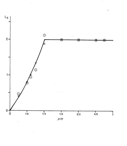
(C^m — 1 ) / (C^m+l — 1)_5n2 X as m —> oo . (2.3.7)

This sequence converges rapidly with increasing m ; in Figure 2.5 we show the estimator Lg as a function of fI together with the value

(2.3.8)

which appears to account for the observed convergence over the whole range except at 11 = k/3. The value, (2.3.8), also agrees with the result obtained for the XXZ chain (Hamer 1986a, Woynarovich and Eckle 1987, Alcaraz, Barber and Batchelor 1987a,b). For p. = tu/3, as in the XXZ chain, we find that the convergence can be accounted for

by assuming that cN ~ 1 + 0 ((fin N )/N 2), where the amplitude is estimated to be approximately 0.83. The physical significance of these results will be discussed in Section 2.3.5.

2.3.2 Mass gap amplitude at criticality

Turning now to the mass gap, (2.3.1), we expect that at criticality (Cardy 1986a) Nkn = 2 7txp + o(l) as N —> oo , (2.3.9)

Figure 2.5 The (negated) exponent o f the leading correction to the conformal

anomaly estimates (2.3.6) and the polarization mass gap (2.3.9) as a function o f 11. The

estimators Lg (Eqn. (2.3.7)) are indicated by the symbol O while x indicates the

corresponding estimate for the mass gap (2.3.9). The anomalous convergence at

[image:42.552.84.498.62.539.2]

29

associated with the polarization and hence we expect

* P =

K — [I

2k (2.3.10)

This result was first established by Nightingale and Blöte (1983) using strips of up to 16 sites. Again, poor convergence was observed at both extremes of (this is particularly evident in Nightingale and Blöte's Figure 1(c)). The result is further supported by the values tabulated in Table 2.4. The corresponding states in the XXZ chain (i.e. states characterized by the same Bethe ansatz zeros), not surprisingly, yield the same exponent (see Section 3.3.2). The results of a similar analysis, as described above for c, to quantify the convergence in (2.3.9), are shown in Figure 2.5, also from strips of width N = 256 and 512. The leading correction to (2.3.9) is again proportional to N“^ with X given by (2.3.8). Again at |i = tc/3, the correction is

logarithmic but now of order (ßn NVN2.

Given data for kn from two different width strips, the critical line can be located

by phenomenological or finite-size renormalization (Barber 1983a, Nightingale 1982); namely by solving the equation

where J 0 is a fixed direction in the parameter space K = ß J. From the point of view of the Bethe ansatz, the most natural implementation of (2.3.11) for the symmetric eight-vertex model involves the variables p and p. with w = 0. Thus we estimate p* (= 0) from the solution pN* of

The resulting estimates for several values of N with N’ = N - 4 are shown in Figure 2.6 as a function of fi.

2.3.3 Phenomenological renormalization - location of Tc

NKN (ß * J0) = N ’KN.(ß * J 0) , (2.3.11)

Nkn (p*,p.) = N 'kN’ (p*,{i). (2.3.12)

<D • s C/3 3 j 0 "äj 1 O c o x : s 05 <u '■I—I j S o> •I Sh o Ü

s

03 ?3 a , <u x ; <+H o c . o o r-j < s S3 M CS t s u. 05 Q-O C 0 ■§ N 1 cl o 'S_g X <u t : <u > w J= Ö0 ‘33 CM

<3

05 rH 00 rv\

5

00 05 c o CO rr\ CO Tf c o rH 05 LO 00 3 M CO CO c o

8 c oc o

r t-H t-H wJ t-H o t-H c o o Uw CO o rH o rH

o

5j

O

rH o rH 3 rH 3

d Ö Ö Ö d d d d d

35

r*5 ofM oCO LO co 05 M c o

rH M '«NM

Ä1 o Mb'

M rHc o GNCO CQc o COCO

LO COwTj

o 'JJ O o CN 00 © VJ oo o CO 00 © CO 00 <3 CO oo o CO 00 COoo

_ft

Ö Ö Ö Ö d d d d Mdb'

CO t> rH o c o c o c o

c-0 5

CO

a

t>

t- 3 s

8

_{8 8 8}

F.

<M LO rH CO CO rH LO

CO COCO

rH CO CO rH CO c o rH CO CO rH CO

c o COCO

Ö Ö Ö Ö d d d TTd rHd

05 M o o

c- c-

05 •

M

s

8

rH

M o00 LO05 0005

8

8

*2

O

c o

j

M

CO

3

05

3

0 5Tt<M

05 Tf M 05 Tf M 05

3

05M LOM

Ö Ö Ö Ö d d d d d

0 5

c o

£

05 COCO COM ₃

£

rHc o £

CO CO CO 00 05 M CO CO o o CO

C— rH CO CO M CO rH £ M CO CO CO CO CO CO £ CO c o c o CO CO CO CO c o c o

Ö Ö Ö Ö d d d d d

rH M 00 T f1 C - t — tr­ 05 t>

CO

C— 8 c orH COT f MrH M e e_LO c o© COc o

c o

r - 3 LOo OrH COrH TfrH LOrH c orH c orH c o

Ö c oÖ Ö

Ö

d d " ' td d Tfl d CN - S _C C3 H m i <M 05 CO 0 0 CO Ö CO O CO rH Ö

O CO M LO

CO O M M

0 0 t > T f CO

0 0 C—■ CO l>*

M CO rH tH

^ ^ HT HT

Ö Ö Ö Ö

o 05 o o LO Ö CM LO Ö CO CO CO 00 LO Ö

£ T f 0 0 CO M

r—H CO 3 00CM

rH 8

(M rH

k2

the theory and hence minimize correction terms that would normally be expected in any realistic finite lattice calculation. A more realistic test is to revert to the magnetic spin formulation and write (2.3.12) as

N i^ (ß*Jia ,o ) ) = N,KN.(ß*J1( l,a ) j , (2.3.13)

where a = K^/Kj is fixed. This conforms with Nightingale's approach (Nightingale 1977, 1979, 1982), although we are using a different gap.

From the parametrization of the vertex weights given in (2.2.41) and their relation to the spin couplings in (2.2.3), the connection between the two formulations can be written

expW K,) = - f.-( >

i2Ux~X

.p )

(2.3.14a)

e x p (4 K ') =

' f 2( / Ä , p )

(2.3.14b)

exp(4K2) = f .

‘ f 2(-X ,p)

(2.3.14c)

At criticality, these equations reduce to

exp(2K 1) = cot(|i/4 - w /4 ), _(2.3.15a)

exp(2K ’1) = cot(p/4 + w /4 ), _(2.3.15b)

e x p ^ i y = ta n p/2 . _(2.3.15c)

2.3.4 Phenomenological renormalization - estimate of v

Let us now turn to the question of estimating the critical exponent v from the phenomenological renormalization group. We have (Barber 1983a,b, 1985)

= r1/v

Vdßj

r I J 0- V%

«V

VtCN/r

* > (2.3.16)

where the asterix indicates that the expressions are to be evaluated at criticality and the gradients are with respect to K. Again choosing N' = N /r = N - 4, we have the estimators

-l

VN 1 +

J 0- Vk

n

)7

J 0-V K N - 4

J2n [N/(N-4)]

(2.3.17)

To extend and clarify the previous finite lattice estimates of v, we consider (2.3.17) as (Nightingale 1982)

- l

VN 1 + Un

d ^n VDjCn^ )

fin [N/(N-4)] (2.3.18)

with, in general, derivatives Di (m) defined by

D- (m) _{, i = 1, 2 (2.3.19)}

The exact result for the thermal exponent can be written as (Baxter 1972, 1982)

yT = v" 1 = j t a n " ‘(exp 2K J = ^ . (2.3.20)

(2.3.21a)

D^m)

D2(m)

1

*

( 2 cosfi 9tc

)

2 sinfi sinfi/2 _{3p sinp/2}

j

4 sin2|i/2

( \ *

dK } (dK }

+ 2 co4i72

9P J _{^ J} (2.3.21b)

Evaluation of critical derivatives

Let us briefly consider the evaluation of the derivatives appearing in (2.3.21). We begin by noting that the derivatives with respect to the variable |i are simply derivatives along the critical line, i.e. marginal derivatives. It is thus convenient to evaluate these derivatives numerically using for example the two-sided, four-point formula

h'(x) h(x-2Ax) - 8h(x-A x) + 8h(x+Ax) - h(x+2Ax) 4

12 Ax + A x). (2.3.22)

The derivatives with respect to the temperature-like variable p are however, derivatives acrossthe critical line (we shall refer to these as thermalderivatives). To use a two-sided derivative as in (2.3.22) we thus need to be able to calculate T0(Q and T ^ Q above the critical temperature.

Fortunately in this formalism, the simple interchange p — p represents the duality transformation between the low- and high-temperature phases of the model. Consider first, the largest eigenvalue T 0(£). The Bethe ansatz equations (2.2.47) involve elliptic functions of nome p2. As none of the zeros characterizing T0(Q are explicitly dependent on p then the duality transformation leaves T0(Q unchanged. We must have

(2.3.23)

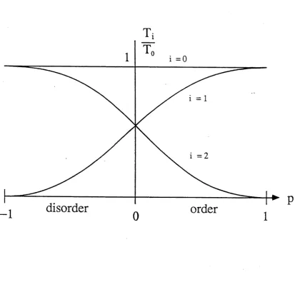
This is indeed the case, the eigenvalue Tj(Q crosses at criticality with the leading eigenvalue in the other sector. We observe that the zero ^ = - p in fact corresponds, in this language, to a 0-string excitation (Johnson et al. 1973). Thus in evaluating the derivative T X(Q at criticality using (2.3.22) we also compute the leading 0-string eigenvalue. This eigenvalue has associated quantum numbers v = v' = v" = 1 and in terms of the original variables in Section 2.2.2 has an exact zero at z1 = - q1/2 (the zero at Zj = - 1 is excited to this position). This level gives in fact, in the spin language, the largest eigenvalue with antiperiodic boundary conditions^. In Figure 2.7 we show these levels schematically as a function of the variable p. We have observed that, in this formalism, quite literally, the whole spectrum can be 'folded over' the vertical line through p = 0.

Alternatively, exact expressions can be derived for the derivatives appearing in (2.3.21), although such expressions involve solving a further set of linear simultaneous equations for the derivatives of the zeros characterizing T0(Q and T X(Q. However, for large N in particular, we have chosen to evaluate the derivatives of the mass gap in this manner. This necessitates only the computation of the zeros characterizing T0(Q and TX(Q at criticality. We derive these equations in Appendix 2D. Finally we mention that we have compared our results for the derivatives in (2.3.21) with the exact "brute force" results for lattice sizes N = 4 and N = 8. We proceed now to our estimates of the critical exponent v.

Numerical Results

As an illustrative example of our results, we show in Figure 2.8a the finite lattice estimates (2.3.18) as a function of the four-spin coupling for the particular value N = 64. Also shown is the direction in which the finite lattice estimates converge to the

t Using (2.2.36), (2.3.1), (2.3.2) and (2.3.8) then gives (5tu/6 - |i)N"2 as the