Non-Linear Observers
Grant Darren Baldwin
October 2009
A thesis submitted for the degree of Doctor of Philosophy
Grant Darren Baldwin
I would like to start by thanking my supervisors Robert Mahony, Jochen Trumpf and
Jonghyuk Kim for their invaluable support, insight, assistance and persistence
through-out my PhD experience. Withthrough-out your confidence and patience the works contained
in this thesis would not have come to fruition. Similarly, I would like to thank Tarek
Hamel for his support and invaluable insights.
Without mentioning names, so that I can’t forget anyone, I extend my thanks to the
students and faculty of the College of Engineering and Computer Science. It has been
a privilege to work in a such an accessible, collegiate and stimulating environment.
You have made it a pleasure to undertake my PhD at the ANU.
I am grateful for financial support received during my PhD from the following
sources:
• Australian Postgraduate Award, funded by the Australian Commonwealth Gov-ernment,
• ANU-NICTA Supplementary Scholarship, funded by National ICT Australia.
This thesis considers the problem of obtaining a high quality estimate of pose (position
and orientation) from a combination of inertial and vision measurements using low
cost sensors. The novelty of this work is in using non-linear observers designed on
the Lie group SE(3). This approach results in robust estimators with strong local and
almost-global stability results and straightforward gain tuning.
A range of sensor models and observer designs are investigated, including
• Creating a cascaded pose observer design using component observers for ori-entation and position, combining pose measurements reconstructed from vision
with inertial measurements of angular velocity and linear acceleration.
• Combining inertial measurement of angular and linear velocity with pose mea-surements reconstructed from vision, and designing an observer using a
decom-position of SE(3)into separate orientation and position components.
• Considering the case where the inertial measurements of angular and linear ve-locity are corrupted by slowly time varying biases and developing an observer
for both pose and velocity measurement bias directly on SE(3)×se(3).
• Eliminating the need for a pose measurement reconstruction by designing an observer operating directly on the measurements of landmark bearing from a
vision sensor. The bearing measurements are combined with unbiased
measure-ments of linear and angular velocity measuremeasure-ments to obtain an observer for
pose evolving on SE(3).
Throughout these works, particular attention is given to designing observers
suit-able for implementation with multiple independent measurement devices. Care is
given to avoid coupling of independent measurement noise processes in estimator
dynamics. Further, the final observers proposed are suitable for a multi-rate
asyn-chronous implementation, making timely use of measurements from sensors whose
measurement rates may differ by over an order of magnitude.
Acknowledgements vii
Abstract ix
1 Introduction 1
1.1 Papers and Publications . . . 3
1.2 Roadmap And Contributions . . . 4
2 Literature Review 7 2.1 Pose Estimation . . . 7
2.1.1 Position Estimation . . . 7
2.1.2 Attitude Estimation . . . 10
2.1.3 Combined Attitude and Position Estimation . . . 14
2.2 Inertial Vision Sensor Systems . . . 15
2.2.1 Pose and Attitude Estimation from Inertial Sensors . . . 16
2.2.2 Pose and Attitude Estimation from Inertial Sensors Augmented with an Additional Exteroceptive Sensor . . . 18
2.2.3 Linear Velocity from Inertial and Exteroceptive Measurements 20 2.2.4 Multi-rate Sensor Fusion . . . 23
2.3 Non-Linear Pose Observers . . . 25
2.3.1 Perspective Systems . . . 26
2.3.2 Observers from Vector and Bearing Measurements . . . 27
2.3.3 Invariant and Symmetry Preserving Observers . . . 27
3 Experimental Apparatus and Methodology 31 3.1 3DM-GX1 Inertial Measurement Unit . . . 32
3.2 Sony XCD X710-CR FireWire Camera . . . 33
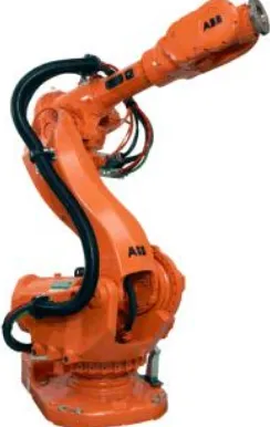
3.3 ABB IRB 6600 175/2.55 Robotic Manipulator . . . 34
3.4 Experimental Environment and Setup . . . 35
3.5 Data Logging Software . . . 37
3.5.1 PC Data Logging System . . . 38
3.5.2 Robot Data Logging System . . . 40
3.6 Data Calibration . . . 40
3.6.1 Measurement Axes and Frame Origins Calibration Protocols . 41 3.6.2 Time Calibration Protocol . . . 43
3.7 Data Pre-Processing . . . 44
3.7.1 Robot Data Pre-Processing . . . 44
3.7.2 IMU Data Pre-Processing . . . 44
3.7.3 Camera Data Pre-Processing . . . 46
3.8 Chapter Summary . . . 49
4 Pose Observer Design onSE(3)by decomposition into Rotation and Trans-lation 51 4.1 Problem Formulation and Measurement Model . . . 53
4.1.1 Problem Formulation . . . 53
4.1.2 Measurement Model . . . 56
4.2 Cascaded Pose Observer . . . 58
4.2.1 Cascaded Pose Attitude Observer . . . 58
4.2.2 Cascaded Pose Position and Velocity Filter . . . 62
4.2.3 Experimental Results . . . 65
4.3 Simultaneous Attitude and Position Filter Design . . . 72
4.3.1 Coordinate Frame Transformation Error Observer . . . 72
4.4 Rigid Body Transformation Error Observer . . . 77
4.5 Zero-Coupling Rigid Body Transformation Error Observer . . . 81
4.5.1 Discrete Integration on SE(3)for Rigid Body Transformation Error Observer . . . 82
4.5.2 Gain selection . . . 84
4.5.3 Simulation Results . . . 85
4.5.4 Experimental Results . . . 90
4.6 Chapter Summary . . . 95
5 Observer Design on the Special Euclidean GroupSE(3) 97 5.1 Problem Formulation . . . 98
5.1.1 Measurement Model . . . 101
5.2.1 Pose and Velocity Bias Observer for Partial Velocity
Measure-ments in Mixed Frames . . . 110
5.3 Observer Implementation . . . 114
5.3.1 Multi-rate Implementation . . . 114
5.3.2 Discretisation . . . 115
5.3.3 Observer Algorithm . . . 116
5.4 Simulation Results . . . 116
5.5 Experimental Results . . . 122
5.6 Chapter Summary . . . 126
6 Observer Design from Direct Vision Measurements of Feature Bearing 127 6.1 Problem Description . . . 128
6.1.1 Measurement Model . . . 131
6.1.2 Estimation Model and Error Terms . . . 132
6.2 Observer Design . . . 134
6.2.1 System Assumptions . . . 134
6.2.2 Landmark Bearing Pose Observer . . . 134
6.3 Simulation Results . . . 139
6.4 Experimental Results . . . 145
6.5 Chapter Summary . . . 150
7 Conclusions 151 A Data Structure Descriptions for Attached Data Sets 171 A.1 Experimental Paths . . . 171
A.2 Raw Data Data Structures . . . 172
A.3 MATLAB Data Structures . . . 173
B Full Proof of Theorem 5.2.1, Chapter 5, Claim (ii): Linearisation of(T˜,b˜Ξ)175 C Observer for Linear Velocity and its Interconnection with Pose Observers183 C.1 Linear Velocity Estimation . . . 183
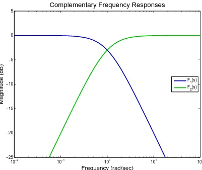
2.1 Illustration of two functions with complementary frequency responses.
At all frequencies,F1(s) +F2(s) =1 (0 dB). . . 19
3.1 Microstrain 3DM-GX1 . . . 33
3.2 Sony XCD 710-CR FireWire Camera . . . 34
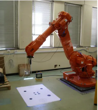
3.3 ABB IRB 6600 175/2.55 robotic manipulator . . . 35
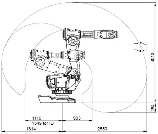
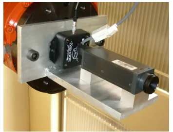
3.4 ABB IRB 6600 175/2.55 robotic manipulator workspace (ABB 2004a) 36 3.5 IMU and camera mount for ABB IRB 6600 . . . 37
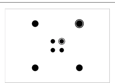
3.6 Visual feature target observed by camera. The target consists of two sets of four features, placed on the vertices of squares with side lengths 50 cm and 10 cm respectively. The first image feature in each square is marked by a double circle and numbering continues clockwise. . . . 38
3.7 Experiment setup, including IRB 6600 with affixed camera and IMU, visual target, lighting, data capture system. . . 39
3.8 Raw acceleration measurements as received from IMU. Note the ap-parent superposition of high magnitude noise on the underlying signal with low magnitude gaussian noise. Similar patterns are observered in gyrometer and magnetometer signal channels. . . 46
3.9 Histogram of norm of acceleration measurement vectors in raw IMU measurements. . . 47
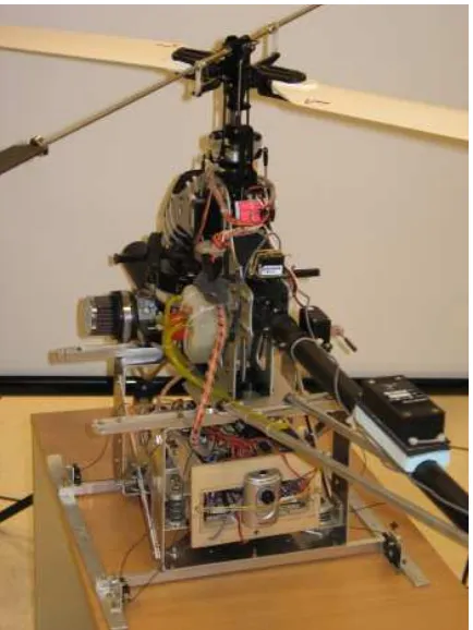
3.10 Acceleration measurements after discarding erroneous measurements 47 3.11 Uncorrected and Corrected low-pass filtered gyrometer measurements. 48 4.1 Experimental platform consisting of a Vario Benzin-Acrobatic 23cc helicopter, low-cost Philips webcam and Microstrain IMU . . . 65
4.2 Estimate of helicopter attitude in the inertial frame produced by Cas-caded Pose Observer using observer gains given in Table 4.1. . . 67
4.3 Estimate of gyroscope biases in the body-fixed frame produced by Cascaded Pose Observer using observer gains given in Table 4.1. . . . 68
4.4 Estimate of helicopter position in the body-fixed frame produced by
Cascaded Pose Observer using observer gains given in Table 4.1. . . . 69
4.5 Estimate of helicopter velocity in the body-fixed frame produced by
Cascaded Pose Observer using observer gains given in Table 4.1. . . . 70
4.6 Estimate of accelerometer biases in the body-fixed frame produced by
Cascaded Pose Observer using observer gains given in Table 4.1. . . . 71
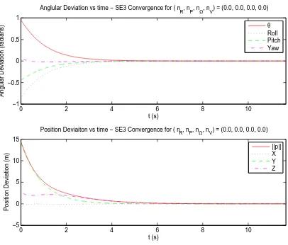
4.7 Simulation result showing attitude and position error in the inertial
frame for Rigid Body Transformation Error Observer using observer
gains given in Table 4.2. Static simulation withΞ=0,T(0)and ˆT(0)
selected randomly and no sensor noise. Typical result from repeated
testing. . . 86
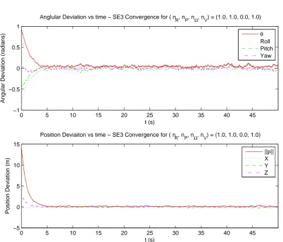
4.8 Simulation result showing attitude and position error in the inertial
frame for Rigid Body Transformation Error Observer using observer
gains given in Table 4.2. Static simulation withΞ=0,T(0)and ˆT(0)
selected randomly and noise variances of 1.0 units on all sensors.
Units for rotation, position, angular and linear velocity respectively
are radians, metres, radians per second and metres per second. Typical
result from repeated testing. . . 87
4.9 Simulation result showing attitude and position error in the inertial
frame for Rigid Body Transformation Error Observer using observer
gains given in Table 4.2. Static simulation withΞ=0,T(0)and ˆT(0)
selected randomly and with noise variance of 1.0 radians per second
on only the angular velocity sensor. Typical result from repeated testing. 88
4.10 Simulation result showing attitude and position error in the inertial
frame for Rigid Body Transformation Error Observer using observer
gains given in Table 4.2. Static simulation withΞ=0,T(0)and ˆT(0)
selected randomly and with noise variances of 1.0 units on all sensors
except the angular velocity sensor. Units for rotation, position and
linear velocity respectively are radians, metres, and metres per second.
4.11 Simulation result showing attitude and position error in the inertial
frame for Zero Coupling Rigid Body Transformation Error Observer
using observer gains given in Table 4.2. Static simulation withΞ=0,
T(0)and ˆT(0)selected randomly and no sensor noise. Typical result
from repeated testing. . . 91
4.12 Simulation result showing attitude and position error in the inertial
frame for Zero Coupling Rigid Body Transformation Error Observer
using observer gains given in Table 4.2. Static simulation withΞ=0,
T(0) and ˆT(0) selected randomly and with noise variance of 1.0 on
only the angular velocity sensor. Typical result from repeated testing. 92
4.13 Estimate of helicopter attitude in the inertial frame produced by Zero
Coupling Rigid Body Transformation Error Observer using observer
gains given in Table 4.3. . . 93
4.14 Estimate of helicopter position in the inertial frame produced by Zero
Coupling Rigid Body Transformation Error Observer using observer
gains given in Table 4.3. . . 94
5.1 The rigid-body transformation from inertial frame,
A
, to the body-fixed frame,B
, is represented byT and the transformation fromA
to the estimation frame,E
, is represented by ˆT. The transformation ˜T, from the body fixed to estimation frames, expressed inA
, is then given by ˆT T−1. . . 103 5.2 Sketch of the geometry of critical points ofL
on SE(3)×R6. On thehalf sphere representing SO(3)we represent the angle of rotation, θ,
by vertical height in the bowl and the two dimensional axis of rotation
by the angular position and heading on the bowl. The bias subspace,
bΞ=R6 and the translational position subspace p=R3 are each at-tached at every point on the bowl, with pbeing attached in different
directions around SO(3) according to the connection on SE(3). The
critical sets(I,0)andU form the base and rim of the SO(3)bowl
re-spectively. Further, in every neighbourhood of every point(TU,0)∈U, there is the initial conditions for a trajectory converging to(I,0). . . . 108
5.3 SE(3) Complementary Filter Block Diagram. Note the structure is
5.4 Simulation results for orientation component of pose estimate using
simulated measurements along a trim trajectory specified by
equa-tion (5.49), with observer gains as per Table 5.1 and initial condiequa-tions ˆ
T(0) =Iand ˆbΞ=0. Artificial measurement noise was added
accord-ing to Table 5.2. The true pose is indicated by red marks and the visual
pose measurements by green marks. Note that while the vision
mea-surements are coincidental with the true pose, they are at a lower rate
of 5 Hz. The estimated pose is indicated by the blue path. . . 119
5.5 Simulation results for position component of pose estimate using
sim-ulated measurements along a trim trajectory specified by equation (5.49),
with observer gains as per Table 5.1 and initial conditions ˆT(0) =I
and ˆbΞ=0. Artificial measurement noise was added according to
Ta-ble 5.2. The true pose is indicated by red marks and the visual pose
measurements by green marks. Note that while the vision
measure-ments are coincidental with the true pose, they are at a lower rate of 5
Hz. The estimated pose is indicated by the blue path. . . 120
5.6 Simulation results for velocity bias estimates using simulated
mea-surements along a trim trajectory specified by equation (5.49), with
observer gains as per Table 5.1 and initial conditions ˆT(0) = I and ˆ
bΞ=0. Artificial measurement noise was added according to Table
5.2. . . 121
5.7 Experimental results for orientation component of pose estimate using
inertial and visual measurements from sensors attached to a robotic
manipulator moved through a circular path. Observer gains used are
given in Table 5.3 and initial conditions were ˆT(0) =Ty(0), ˆbΞ=0.
The estimated pose is indicated by the blue path and visual pose
mea-surements by green marks. The ground truth meamea-surements of the
5.8 Experimental results for position component of pose estimate using
inertial and visual measurements from sensors attached to a robotic
manipulator moved through a circular path. Observer gains used are
given in Table 5.3 and initial conditions were ˆT(0) =Ty(0), ˆbΞ=0.
The estimated pose is indicated by the blue path and visual pose
mea-surements by green marks. The ground truth meamea-surements of the
actual path recorded by the robot are indicated by the red marks. . . . 124
5.9 Experimental results for velocity bias estimates using inertial and
vi-sual measurements from sensors attached to a robotic manipulator
moved through a circular path. Observer gains used are given in Table
5.3 and initial conditions were ˆT(0) =Ty(0), ˆbΞ=0. . . 125
6.1 The true system state,T, contains the rotation and translation from the
origin of the inertial frame,
A
, to the origin of the body fixed frame,B
. The landmarks have locationziin the inertial frame and are observedfrom the body fixed frame. . . 130
6.2 The true system state,T, contains the rotation and translation from the
origin of the inertial frame,
A
, to the origin of the body fixed frame,B
. The landmarks have locationziin the inertial frame and are observedfrom the body-fixed frame as bearingsXi, represented on the unit sphere.131
6.3 Simulation results for orientation component of pose estimate using
simulated measurements along a trim trajectory specified by
equa-tion (6.38), with observer gains as per Table 6.1 and initial condiequa-tions ˆ
T(0) =I. Artificial measurement noise was added according to Table
6.2. The true pose is indicated by red marks and the visual pose
mea-surements by green marks. Note that while the vision meamea-surements
are coincidental with the true pose, they are at a lower rate of 20 Hz.
6.4 Simulation results for position component of pose estimate using
sim-ulated measurements along a trim trajectory specified by equation (6.38),
with observer gains as per Table 6.1 and initial conditions ˆT(0) =I.
Artificial measurement noise was added according to Table 6.2. The
true pose is indicated by red marks and the visual pose measurements
by green marks. Note that while the vision measurements are
coin-cidental with the true pose, they are at a lower rate of 20 Hz. The
estimated pose is indicated by the blue path. . . 142
6.5 Simulation results for orientation component of pose estimate for large
initial condition error, using simulated measurements along a trim
tra-jectory specified by equation (6.38), with observer gains as per Table
6.1 and initial conditions given in equation (6.39). Artificial
measure-ment noise was added according to Table 6.2. The true pose is
indi-cated by red marks and the visual pose measurements by green marks.
Note that while the vision measurements are coincidental with the true
pose, they are at a lower rate of 20 Hz. The estimated pose is indicated
by the blue path. . . 143
6.6 Simulation results for position component of pose estimate for large
initial condition error, using simulated measurements along a trim
tra-jectory specified by equation (6.38), with observer gains as per Table
6.1 and initial conditions given in equation (6.39). Artificial
measure-ment noise was added according to Table 6.2. The true pose is
indi-cated by red marks and the visual pose measurements by green marks.
Note that while the vision measurements are coincidental with the true
pose, they are at a lower rate of 20 Hz. The estimated pose is indicated
by the blue path. . . 144
6.7 Experimental results for orientation component of pose estimate using
inertial and visual measurements from sensors attached to a robotic
manipulator moved through a circular path. Observer gains used are
given in Table 6.3 and initial conditions were ˆT(0) =Ty(0), ˆbΞ=0.
The estimated pose is indicated by the blue path and visual pose
mea-surements by green marks. The ground truth meamea-surements of the
6.8 Experimental results for position component of pose estimate using
inertial and visual measurements from sensors attached to a robotic
manipulator moved through a circular path. Observer gains used are
given in Table 6.3 and initial conditions were ˆT(0) =Ty(0), ˆbΞ=0.
The estimated pose is indicated by the blue path and visual pose
mea-surements by green marks. The ground truth meamea-surements of the
actual path recorded by the robot are indicated by the red marks. . . . 148
6.9 Experimental results for velocity bias estimates using inertial and
vi-sual measurements from sensors attached to a robotic manipulator
moved through a circular path. Observer gains used are given in Table
3.1 Extract of 3DM-GX1 Detailed Specifications (Mic 2006b). . . 33
3.2 List of software libraries used by data logging system . . . 40
4.1 Observer gains used in flight experiment with SO(3)×R3observer. . 66
4.2 Observer gains used in simulations depicted in Figures 4.7, 4.8, 4.9,
4.10, 4.7 . . . 85
4.3 Observer gains used experimental results with Zero Coupling Rigid
Body Transformation Error Observer . . . 90
5.1 Observer gains used in simulations depicted in Figures 5.4, 5.5 and
5.6. . . 118
5.2 Artificial noise and bias figures applied to measurements in
simula-tions depicted in Figures 5.4, 5.5 and 5.6. . . 118
5.3 Observer gains used in experiments depicted in Figures 5.7, 5.8 and
5.9. . . 122
6.1 Observer gains used in simulations depicted in Figures 6.3, 6.4, 6.5
and 6.6. . . 140
6.2 Artificial noise figures applied to measurements in simulations
de-picted in Figures 6.3, 6.4, 6.5 and 6.6. . . 140
6.3 Observer gains used in experiments depicted in Figures 6.7, 6.8 and
6.9. . . 146
Introduction
Accurate, high-rate estimation of attitude and position is important to many areas of
robotics. For example, in the control of autonomous vehicles and the callibration of
sensing systems. Such system can usually be modelled as rigid body kinematics and
dynamics, where the pose lies naturally in the group of rigid body transformations, the
special Euclidean group SE(3) of dimension four. The problem of pose estimation,
and attitude estimation in general, is known to be a highly non-linear problem due to
the geometry of rotations in three dimensional space (e.g. Murray et al. 1993). For the
estimation of attitude alone, a wide range of techniques have been proposed including
Kalman filter variants, particle filters and non-linear observers (Crassidis et al. 2007),
each with different merits.
Localization, the process of estimating the position and attitude of an object
rel-ative to an operating environment, is thought to occur in humans through a fusion of
predictive information from proprioceptive senses, such as the vestibular system in
the inner ear, with corrective information from exteroceptive senses, such as sight and
hearing. Information from the vestibular system provides an estimate of how our
po-sition and attitude have changed, measuring quantities such as angular velocity and
acceleration, including gravity, experienced by the head. This information is sufficient
for short term state estimation, using an approximate integration of measurements, but,
as anyone who has attempted to walk through a room in the dark will notice, does not
provide a good long term estimate. Fusing the information from the vestibular with
estimates of our surroundings from vision and auditory sensors, and other senses such
as touch, provides correction of drift in vestibular estimates.
Similarly, one may estimate the position and attitude, or pose, of a robotic
vehi-cle by fusing the output of multiple sensors. The principal reason for doing this is
to combine measurements from disparate sensors with different desirable
characteris-tics, such as a high measurement rate or high accuracy, to obtain a resulting estimate
that combines the desirable properties of several separate sensors. Additionally,
multi-ple independent measurements provide a way of reducing the effects of measurement
noise, and fusion may be used to create a composite measurement from sensors each
only partially measuring an input or output to a system.
A wide range of sensors, with varying noise and disturbance characteristics, may
be used to measure the inputs and outputs of this system, either in full or part. For
ex-ample, an array of gyrometers measures angular velocity, a Global Positioning System
(GPS) device measures attitude and position, and a receiver for an ultrasonic beacon
may measure distance from the beacon; a component of position.
A particular sensor combination of recent scientific interest is the combination
of an inertial sensor package with a vision sensor, a combination referred to as an
inertial-vision sensor system. An inertial sensor package is functionally similar to the
human vestibular, providing measurements of angular velocity and linear acceleration,
commonly at a very high rate, exceeding 100 Hz, but with undesirable measurement
disturbances, especially in low-cost models. A vision sensor, such as a common
we-bcam or digital camera, observes a two dimensional projection of the environment of
the vehicle from which, under certain conditions, the pose of the sensor can be
calcu-lated. Typically a vision sensor measures at low rates of 30 Hz and below, but with
very small, and in particular unbiased, measurement disturbance.
Inertial-vision sensor packages are of scientific interest for several reasons,
includ-ing the low cost of the sensor combination, the possibility of multi-modal use of vision
sensors, and the relationship to human perception. Some techniques for estimation
from inertial-vision sensors also support use of other sensors in the place of vision,
such as GPS or ultrasonic triangulation.
This thesis considers the problem of obtaining high quality, high rate estimates of
attitude and position, or pose, from a combination of inertial and vision measurements
using low cost sensors. In particular, it will consider the fusion of high frequency
iner-tial measurements with low frequency vision measurements to obtain a robust, precise
and accurate pose estimation updated at the high measurement rate of the inertial
sen-sor.
The approach taken it to investigate the use of non-linear observers for pose
estima-tion, with particular emphasis given to designing observers on SE(3), a mathematical
construct encapsulating the natural geometry of the problem. Prior work applying
sta-bility proofs and show great promise for future applications (Crassidis et al. 2007).
Work presented in this thesis commences by extending work attitude estimation using
non-linear observers presented in Mahony et al. (2008).
The research documented considers a range of sensor modalities for both the
iner-tial and vision sensor, and will principally consider the case of onboard sensors. Work
includes consideration of both biased and unbiased inertial sensor measurements.
The research documented in this thesis focuses on the design of estimators that are
robust to measurement distrubances, have a wide basin of attraction and are simple to
implement and tune. These criteria are aimed at being competitve the robustness and
accuracy of techniques such as Kalman filtering, while adding additional properties
and simplifying their use.
Specifically, this research seeks to produce estimators that are:
• Robust to measurement disturbances, including insensitivity to Gaussian noise and correction of measurement biases.
• Insensitive to initial condition error;
• Capable of being implemented to operate at the rate of the fastest measurement, preferably without requiring regular measurement timing;
• Straightforward to tune, preferably with few scalar gains and demonstrated sta-bility across a wide range of gain values;
• Backed by formal mathematical proof of stability for the continuous time case with no measurement noise.
This thesis includes both simulation and experimental validation of proposed
ob-servers, including generation of indigenous experimental data sets.
1.1
Papers and Publications
This thesis includes work contained in the following academic papers
• Cheviron, T.; Hamel, T.; Mahony, R. and Baldwin, G. Robust Nonlinear Fu-sion of Inertial and Visual Data for position, velocity and attitude estimation
of UAV. InProceedings of the 2007 IEEE International Conference on Robotics
• Baldwin, G.; Mahony, R.; Trumpf, J.; Hamel, T. and Cheviron, T. Complemen-tary filter design on the Special Euclidean group SE(3), InProceeding of the
European Control Conference 2007, Kos, Greece, July 2007.
• Baldwin, G.; Mahony, R.; Trumpf, J. and Hamel, T.Complementary Filtering on the Special Euclidean Group. Submitted toIEEE Transactions on Robotics,
2008.
• Baldwin, G.; Mahony, R. and Trumpf, J. A Nonlinear Observer for 6 DOF Pose Estimation from Inertial and Bearing Measurements. In Proceedings
of the 2009 IEEE International Conference on Robotics and Automation, Kobe,
Japan, May 2009. 2237–2242.
1.2
Roadmap And Contributions
This thesis comprises seven chapters including this introduction.
• Chapter 2 is a literature review that surveys the body of scientific work on pose estimation, the use of inertial-vision sensors in pose estimation and
develop-ments in non-linear observers relevant to pose estimation.
• Chapter 3 describes the systems and protocols used for the collection of ex-perimental data from an inertial-vision system for exex-perimental validation of
observers presented in this thesis. Notably, this system, based on a large, 2 m
reach, robotic arm includes measurement of ground-truth reference data against
which estimates can be compared.
• Chapter 4 presents two approaches to designing a non-linear pose observer by making use of a decompositions that permit independent design of the rotation
and position components. The first approach presented comprises independent
attitude and position observers, with the attitude estimate used as an input for
the position observer for which stability is proven in the presence of an
expo-nentially decaying input disturbance resulting from the cascade. The second and
third approaches design the rotation and position estimation components
simul-taneously but within a single observer by decomposing a Lyapunov function into
• Chapter 5 describes the design of an observer for both pose and velocity mea-surement biases. An almost-global asymptotic and locally exponential
Lya-punov stability proof is given together with an extension to the case where
ve-locity measurements are measured in two orthogonal components in different
frames of reference with separate bias processes. Implementation issues are
ad-dressed including presentation of a sample discrete time algorithm.
• Chapter 6 presents a pose observer that uses projective vision measurements of bearing from the camera to a landmark, instead of vision measurements of pose.
This corresponds to a simpler, more direct use of vision measurements without
requiring complicated post processing. Again, a Lyapunov stability argument
is given, proving local asymptotic stability. Based on work in Chapter 5, the
observer is extended to address velocity bias estimation.
• Chapter 7 conclude this thesis, summarising the results of this research.
Experimental data and MATLAB scripts implementing the observers described in
this thesis are contained in an attached DVD. Additionally, this thesis contains three
appendicies describing the contents of the attached DVD and providing further results
not included in the main text.
• Appendix A contains descriptions of the contents of the DVD atttachement to this thesis, including raw and pre-processed data sets from experiment series
reported in this thesis.
• Appendix B provides the full proof of a linearisation argument using in Theorem 5.2.1 of Chapter 5.
• Appendix C presents a sample observer for linear velocity from measurements of pose, angular velocity and linear acceleration in the presence of inertial
mea-surement biases. By use of such an observer, one can treat an appropriate
iner-tial sensor as providing measurements of the system velocity, angular and linear.
Appendix C also outlines sufficient conditions for ensuring the cascade of a
Literature Review
In this chapter I will critically review the background literature relevant to the problems
considered in this thesis. Section 2.1 reviews historical approaches to the problems of
estimating position, attitude and pose. Section 2.2 provides an overview of inertial
vi-sion sensor packages and a summary of prior work utilising them for attitude and pose
estimation. Finally, Section 2.3 surveys prior work in the use of non-linear observers
for the estimation of pose and attitude.
2.1
Pose Estimation
Accurate estimation of the attitude and position of a vehicle is vital to many areas of
scientific endeavour, including navigation, robotics and automation. In this section, I
present a review of common practices and techniques for the estimation of attitude and
position independently, and for their combined estimation as pose.
Position estimation in a static frame of reference is a linear problem which can
be tackled by well studied techniques such as Kalman filtering. Attitude estimation
is however a highly non-linear problem requiring different techniques. Estimation of
both position and attitude by a single estimation system may be simultaneous in a
single estimator, or through a cascade of the results from one estimator into another.
2.1.1
Position Estimation
The standard representation for the position of an object in three dimensional space
is as a three-vector, p∈R3. In a non-rotating, inertial, frame, p has the customary kinematics
˙ p=v
˙ v=a
(2.1)
wherevis linear velocity and athe acceleration, both also three-vectors inR3. With measurements of p, v ora, or full rank linear combinations thereof, estimating p is
then a linear problem.
Estimating position based measurements ofp,vora, or linear combinations thereof,
is a self-evidently important problem with applications including navigation, robotics
and automation.
2.1.1.1 Asymptotic Observers
One of the simplest methods for defining an estimator for a linear problem is the
asymptotic observer (see e.g. Kailath et al. 2000). For the general linear system with
statex, input signalu, outputyand kinematics
˙
x=Ax+Bu
y=Cx
(2.2)
whereA, BandC are known, full rank, matrices, one can define the estimate ˆx with
kinematics
˙ˆ
x=Axˆ+Bu+K(y−Cxˆ) (2.3)
from measurements ofuand y. By selecting the matrixK6=0 such that (A−KC)is Hurwitz, one can ensure the estimation error, ˜x=xˆ−xwill asymptotically converge to zero based on the error kinematics ˙˜x= (A−KC)x. Further, the rate of convergence is˜ defined by the eigenvalues of(A−KC). A matrix Kcan always be selected to ensure
(A−KC)is stable provided the system in equation (2.2) is detectable. By application of the pole placement theorem, observability of {A,C} is a sufficient condition for detectability (e.g. Polderman and Willems 1998).
Consider a cost function on the state estimate error of the form
L
=x˜>Px˜, (2.4)where(·)> denotes the matrix transpose,Pis a symmetric, positive definite matrix.
L
is a quadratric cost function measuring the deviation of ˜xfrom 0. Lyapunov stabilitytheory (e.g. Khalil 2002, Slotine and Lie 1991, Rouche et al. 1977) provides the result
that stability of the linear time invariant system ˜x is equivalent to the existence of
symmetric positive definite matrix P for any choice of symmetric positive definite
theory introduces the notion of exponential stability, where the value of a cost function
on the state is bounded above by a decaying exponential in time.
Note that as an observer, acting on ideal noise free measurements and unrestricted
by innovation energy constraints, it is often possible to make the eigenvalues of(A− KC)arbitrarily large and hence convergence of the error to 0 arbitrarily fast.
Further, consider the case where the inputuand measurementsyare corrupted by
independent additive white Gaussian noise processes, and hence ˆxis random variable
whose covariance is related to the covariances ofu andy. Correspondingly ˜x is also
a random variable with the same covariance, and the quadratic cost
L
is likewise a random variable with a mean related to the covariance of ˜x. Setting the design goalof estimating ˆx such that ˜x is zero mean with minimum covariance, minimising the
mean of
L
, one has a Linear Quadratic Gaussian system for which we are attempting to construct a Linear Quadratic Estimator.2.1.1.2 Linear Kalman Filters
There exists a single optimal estimator for a Linear Quadratic Gaussian system, the
Kalman filter (Kalman 1960, Kalman and Bucy 1961). The Kalman filter has been the
subject considerable research and many publications over the past 50 years, including
analysis and formulations for both discrete and continuous systems. For a detailed
analysis see, e.g., Anderson and Moore (1979), Kailath et al. (2000).
Resembling the asymptotic observer for the case of noiseless measurements,
equa-tion (2.3), the Kalman filter adds an algorithm for selecting an optimal gain matrix at a
given time,K(t), based on solving an algebraic Riccati equation that includes
estimat-ing the measurement covariance based on the time history of measurements received
so far. The optimal gainK(t)is chose such that the expected value of quadratic cost
function is minimised, subject to estimates measurement uncertainty. In the Kalman
filter, this is broken down into a predictor and a corrector step at each update. In the
predictor step, the covariance and state estimates are propagated based on the input
and state dynamics. In the corrector step, the optimal gain computed and innovation
terms applied to state and covariance estimates.
Linear Quadratic Gaussian systems form a fundamental and widely studied
com-ponent of control theory as they model many natural systems, such as position and
ve-locity estimation from noisy inertial measurements, and a simple class of systems that
linear in a sufficiently small area about its operating point. Further, additive white
Gaussian noise is an accurate model of sensor noise process arising from sources such
as transmission of analogue waveforms (e.g. Couch 2001, Proakis and Salehi 2001).
2.1.2
Attitude Estimation
Attitude estimation is an inherently non-linear problem. Unlike the linear problem
of position estimation, which occurs on a vector space, attitude estimation occurs on
a curved, compact group. Specifically, attitude estimation for objects in three
dimen-sional space occurs on the special orthogonal group SO(3)of dimension four, a smooth
differentiable manifold. The group SO(3) contains every unique rotation that can be
applied to a vector inR3, including the identity, or rotation by 0 degrees, and the in-verse for every rotation. Further, as the angle of rotation passes 180 degrees, the group
loops back on itself, giving it its compact property.
Attitude estimation is vitally important for trade, commerce and military
appli-cations. In ancient times, the attitude of a ship on the oceans surface was estimated
using a magnetic compass and measurements of the stars. Precise estimation of the
ships attitude was vital to reaching safe ports and avoiding nautical dangers, especially
when out of sight of coastal references. In more recent times, air and spacecraft have
extended the need to precise attitude estimation in three dimensions and at high
fre-quency. For aircraft in particular, attitude estimation is vital to their safe operation.
Without an accurate estimate of attitude, aircraft risk not only drifting off-course, but
loss of control, stalls and crashes.
A number of distinct techniques have been applied to the problem of attitude
esti-mation over the course of the last century, ranging from extensions of linear estiesti-mation
algorithms to novel non-linear techniques. These techniques have both been driven by
and driven the development of accurate and high-performance air and spacecraft,
es-pecially autonomous vehicles. Common sensor used in estimation include inertial,
magnetic field, vision and Global Positioning System (GPS) sensors.
Crassidis, Markley and Cheng present a comprehensive survey of attitude
esti-mation techniques with particular emphasis on the practicality of each technique in
real-world applications (Crassidis et al. 2007). This survey focuses heavily upon
Ex-tended Kalman Filter (EKF) based techniques, which have been long established as the
workhorse of non-linear estimation (e.g. Allerton and Jia 2005, Armesto et al. 2004,
Trawny et al. 2007, Mourikis et al. 2007, Mourikis and Roumeliotis 2007, Bonnabel
2007). The survey also considers newer techniques including unscented filters (e.g.
Julier and Uhlmann 2002a,b, Wan and van der Merwe 2000), particle filters (e.g.
Cheng and Crassidis 2004, Gustafsson et al. 2002, van der Merwe et al. 2000), and
non-linear observers (e.g. Thienel and Sanner 2003, Thienel 2004, Hamel and
Ma-hony 2006, MaMa-hony et al. 2008, 2005).
Other surveys on the topic of attitude estimation include Lefferts et al. (1982),
Allerton and Jia (2005) and Meng et al. (2008).
2.1.2.1 Extended Kalman Filters
The Extended Kalman Filter (EKF) refers to a family of estimators in which
non-linear systems are locally approximated by non-linear quadratic Gaussian systems and their
state estimated using the Kalman filter. For a given non-linear system there are many
ways of obtaining and maintaining a local linear approximation of the state and input
dynamics. Commonly, the local linear estimate will be taken about the current best
state estimate using a linearisation chosen for accuracy over an area proportionate to
the rate at which the linearisation is updated.
In the problem of attitude estimation, the linearised state is commonly represented
using Euler angles (e.g. Craig 1989), Rodrigues parameters (e.g. Murray et al. 1993)
or unit quaternions (again, e.g. Murray et al. 1993). Each approach has advantages
and disadvantages in terms of the state and input dynamics. In particular, any three
dimensional representation of attitude, such as Euler angles and Rodrigues parameters,
necessarily has at least one singular point near which state representations must be
shifted to avoid singularity.
2.1.2.2 Unscented Kalman Filters
A key performance limitation of an EKF is the region of validity for the linearisation
(Julier and Uhlmann 1997). For highly non-linear problems, such as attitude
estima-tion for aircraft, the region of validity of the linearisaestima-tion of the state dynamics in
the update step may be significantly smaller than the movement of the state trajectory
over the update time step causing the evolution of the state dynamics to be incorrect
and ill-defined. This can be alleviated by raising the rate at which the linearisation is
Further, Julier and Uhlmann observe that under the repeated linearisation of the
EKF, the state estimates can become statistically biased and inconsistent due to the
Taylor series truncation inherent in the linearisation (Julier and Uhlmann 1997). That
is, the state estimate can be incorrect, or biased, and the covariance estimate
underes-timated, or inconsistent. This combination can cause the filter to diverge.
Julier and Uhlmann propose an alternative in the Unscented Kalman Filter (UKF)
(Julier and Uhlmann 1997, Julier et al. 1995). While the EKF handles nonlinear
dy-namics by linearising the problem about the operating point, the Unscented Kalman
Filter (UKF) uses a non-linear transformation of a set of carefully selected points from
a Gaussian distribution
The UKF replaces the EKF prediction step, where state and covariance estimates
are propagated via linearised system dynamics, with a novel estimation scheme based
on the true non-linear trajectory for a set of points characterising the state and
covari-ance distribution, a process called the unscented transformation. A set of point, called
sigma points are selected to represent the state and covariance estimate. These points
are usually initialised as being along basis directions of the covariance, at a distance of
the standard deviation from the mean. For each prediction step, the location of these
sigma points is predicted using the true non-linear state dynamics function, and from
these predicted sigma points the state and covariance after the time step estimated.
Using the true non-linear function of state dynamics rather than a linearisation allows
estimation of the state and covariance at up to second order for state and third order for
covariance, compared with the first order estimate obtained by the EKF. The corrector
step remains the same in the UKF.
Sigma-point based estimators offer several advantages over EKFs. The Unscented
transformation is statistically both unbiased and consistent, compared with the biased
and inconsistent result obtained using the linearisation to propagate the state and
co-variance estimates. Additionally, eliminating the need to compute analytic Jacobians
for the linearised system dynamics significantly reduces the computational cost of each
iteration.
2.1.2.3 Particle Filters
Particle filters have also successfully applied to the attitude estimation problem (e.g.
Cheng and Crassidis 2004, Oshman and Carmi 2004a,b). Particle filters form a large
in which the state probability density function is approximated using point samples
distributed pseudo-randomly according to the prior distribution (Doucet et al. 2001,
MacKay 2003). At each iteration of the filter, the particle locations are updated using
drift, diffusion and resampling processes. After estimation, the particles are let ‘drift’
down gradient directions towards local maxima in the state distribution. To prevent
a degenerate case, particles are also ‘diffused’ using a random walk, and a subset
of particles resampled; redistributed pseudo-randomly using the current distribution
estimate. Particle filters can differ substantially in the algorithms used for diffusion,
drift and resampling point selection, in addition to the number of particles and state
representation. Scaling the number of particles used can greatly vary the accuracy and
computational efficiency of the filter.
For strongly non-linear and non-Gaussian problems, particle filters can prove
su-perior to conventional nonlinear filters, such as from the Kalman filter family. In
par-ticular particle filters are able to estimate multi-modal distributions and, due to the
resampling and diffusion processes, are able to cope with local minima.
The two major drawbacks to the particle filter are its inherent suboptimality and
computational cost on high dimensional problems. The structure of a particle filter is
inherently suboptimal due to the diffusion and resampling processes. As the
dimen-sionality of the problem increases, the number of particles required to approximate the
distribution increases with the power of the dimension (Daum and Huang 2003, Oh
1991).
2.1.2.4 Other Solutions to Attitude Estimation
In addition to the application of generic non-linear estimation methods, there have
been attempts to develop methods of attitude estimation using the specific properties
of the non-linear attitude estimation problem. Of note is the Quaternion Estimator
(QueST) (Shuster and Oh 1981), a method based on Wahba’s problem (Wahba 1965),
which is to find the orthogonal matrix R that minimizes the mean squared error
be-tween observations of reference vectors,Zyi, and estimates of the vector measurements,
Rzi. QueST solves Wahba’s problem using a fading memory of previous estimates to
smooth process noise. The QueST algorithm includes elements from optimal
2.1.2.5 Non-Linear Observers
A comparatively recent approach has been the use of an asymptotic observer structure
constructed on a non-linear space, in this case SO(3), to provide estimates of attitude
(Thienel and Sanner 2001, 2003, Thienel 2004, Thienel and Sanner 2007, Hamel and
Mahony 2006, Mahony et al. 2008, 2005, Bonnabel et al. 2006b, Vasconcelos et al.
2007).
Non-linear observers offer significant advantages in the simplicity of
implemen-tation and tuning, and robustness to measurement noise. As they are often
accompa-nied by global or almost-global stability proofs, many non-linear observers may be
initialised with almost any initial conditions and will reconverge after an almost
ar-bitrarily bad noise injection. In addition, many non-linear observers are also locally
exponentially convergent, dominating most unbiased measurement noise processes.
The almost-global nature of the stability proofs for non-linear attitude observers is
an unavoidable consequence of working on SO(3). Due to the compact structure of
SO(3)there necessarily exists an antipodal set in which multiple directions are
equi-distant from the goal attitude, such that the vector sum of paths to the goal is zero.
Often, this set corresponds to the set of all orientations a rotation ofπradians from the
goal about any axis. This set necessarily has measure zero.
Many non-linear observers commonly feature a small number of gains, with
con-vergence for a wide range of gains, if not all gains. Even with discrete implementation
the range of values for which the observer is convergent can cover several orders of
magnitude, significantly simplifying the tuning process.
It is noted by Crassidis et al. (2007) that these newer, non-EKF based approaches
have demonstrated several advantages over EKF approaches, particularly as non-linearity,
non-Gaussian statistics and poor a-priori state estimates become problematic. In
par-ticular, Crassidis et. al. note that although non-linear observers are still in their infancy,
these methods show great promise for future applications.
2.1.3
Combined Attitude and Position Estimation
For many applications, including navigation and automation, it is necessary to estimate
both the attitude and position of a vehicle. The two may be treated as separate
esti-mation problems, or combined into a single estiesti-mation problem, where one estimate
by a single estimator.
With many practical sensor system, independent estimation is not possible as the
system model couples the attitude and position components, such as when measuring
linear velocity or acceleration in a body-fixed frame and needing rotate it into an
in-ertial frame. In such a case, an estimate of the rotation from the body-fixed to inin-ertial
frame may be produced by an attitude estimator and used as an input to a position
es-timator. This sort of two-stage estimation structure is referred to as a cascade system.
The stability of the estimate ˆpwill depend upon the stability of its input, the estimate ˆ
Rand upon the ability to estimator p to handle non-Gaussian perturbation in this
in-put. One approach to proving stability in this case is to use theorems on input-to-state
stability (Sontag and Wang 1995, Sepulchre et al. 1997).
An alternative is to simultaneously estimate position and attitude using a single
estimator. In this case one defines a state vector containing both attitude and position,
and defines appropriate state and input dynamics. When used in an extended Kalman
filter structure, as in e.g. Kim et al. (2007) or Huster and Rock (2001), this offers
the advantage over a cascade solution of organically estimating covariances arising
from attitude-position interaction. However, it suffers the notable drawback of being a
higher dimensional state space that must be linearised.
Huster and Rock (2003) note that for particular sensor configurations, including
the monocular camera plus inertial sensor considered in this thesis, an EKF approach
exhibits a number of deficiencies. They note substantial error accumulation in the state
covariance matrix due to repeated linearisation, leading to biased estimates.
Specif-ically, the EKF does not account for uncertainty in the construction of linearisations
arising from uncertainty in state estimates.
Other approaches to simultaneous attitude and position estimation include
tech-niques based on the unscented transformation of the unscented Kalman filter (e.g.
Huster and Rock 2003), particle filters (e.g. Vernaza and Lee 2006), and other
sta-tistical estimators (e.g. Kong 2004).
An area of deficit in the literature until recently has been in the application of
non-linear observers to pose estimation, in particular where the observer is posed as a
system evolving on the special Euclidean group SE(3)of dimension four. SE(3)is a
differentiable manifold and Lie group naturally representing the motion of rigid bodies
as an attitude and position with corresponding kinematics (see e.g. Murray et al. 1993,
design to make use of the natural geometry of the estimation problem. Recent work
in this area includes Martin et al. (2004), Bonnabel and Rouchon (2006), Vasconcelos
et al. (2007), Martin and Sala¨un (2008a), Bonnabel et al. (2009a) and this thesis. This
area of literature will be examined in detail in Section 2.3.
2.2
Inertial Vision Sensor Systems
Most estimators for attitude and pose, such as the observers and Kalman filter
de-scribed in Sections 2.1.1 and 2.1.2, feature estimate dynamics that include both
mea-surements of system input and outputs. Using the inputs, the system state is predicted
and from comparing the outputs of the true system to those of the estimate, the estimate
is corrected.
For a rigid body dynamical system, the inputs to motion are the velocities, forces
or accelerations applied and the outputs the attitude and position of the system. Each
of these may be measured directly or as some function of the input or output, such
as measuring the operating point of a thruster and using that to estimate the forces
applied.
A common and widely available sensor package for velocity and acceleration is an
IMU, providing measurements of angular velocity and linear acceleration. The cost,
availability, accuracy and uniform utility of inertial sensors generally dominates any
alternatives such as force estimation from thrust.
For attitude and position common sensors include vision and those based on
tri-angulation from received signals, such as GPS or sonar localisation. Tritri-angulation
for received signals requires an operating environment where the signals can be
re-ceived in a clear and unadulterated manner for optimal accuracy; reflections, noise and
delayed transmission can cause considerable error in pose measurements. This means
that systems such as satellite based GPS are not always reliable in indoor, urban canyon
or other cluttered environments. Vision sensors do not suffer this limitation as their
measurements are reliant only on reflected visible light.
Typical vision sensors, such as the standard pinhole camera model, observe a two
dimensional projection of the scence in front of the camera. If certain details of the
scene are known, such as the position of several objects, the pose of the camera may
be calculated using the position of the features corresponding to those objects in the
a sensor for both attitude and position. Additionally, the location of individual features
in the projected image, or calculations of visual flow between images may also be used
as measurements of the system output in an estimation.
In this thesis, I concentrate on the estimation of pose using the combination of an
inertial sensor and a vision sensor. This combination, often referred to as an
inertial-vision sensor package, provides measurements of both the inputs and outputs of a
rigid body motion system. An inertial-vision sensor package has several desirable
characteristics, including complementary noise spectra between component sensors,
the option of pursuing high-rate estimate, the possibility of multi-modal use of the
vision sensor and low weight and cost requirements.
The use of inertial-vision sensor packages has been of recent interest to the
sci-entific community, with two workshop (Vincze et al. 2003, Corke et al. 2005) and
a tutorial (Dias and Lobo 2008) at recent major international conferences, and with
associated journal special issues.
2.2.1
Pose and Attitude Estimation from Inertial Sensors
Inertial sensor packages contain a series of discrete sensors providing measurements of
angular velocity, linear acceleration, magnetic field and inclination. A typical inertial
sensor package, such as the 3DM-GX1 (Mic 2006b) may contain up to 9, and in some
cases more, discrete sensors; 3 each of gyroscopes, accelerometers and magnetomers,
one of each aligned to a different cardinal direction, plus other auxilliary sensors.
Using a high quality Inertial Measurement Unit (IMU) pose may be estimated from
inertial sensors alone, by direct integration of measurements. This process, known as
dead reckoning, has been used for navigation in cases where exteroceptive sensors are
unavailable, such as submarines and strategic missiles. This process is used in the
original Inertial Navigation Systems (INSs), a technology brought to maturity during
the development of nuclear submarines and theatre ballistic missiles in the 1960’s.
Accurate dead reckoning relies on the use of highly precise, well calibrated and, by
necessity, expensive inertial sensors, as integration of noise and bias errors can rapidly
accumulate, causing the state estimate to diverge.
In many modern guided munitions and delivery systems, inertial navigation is used
as a component of the guidance systems. Modern sensors used in such systems
in-clude ring laser gyroscopes and quartz resonance accelerometers. Such sensors are
For example, the Joint Direct Attack Munition (JDAM), designed as a cheap guidance
system for existing inventories of unguided gravity bombs, and which has an accuracy
of 30 m over a course of up to 15 miles on inertial navigation alone, has been priced
at US$18,000 per unit, (GlobalSecurity.org 2006, Federation of American Scientists
2008), of which the inertial nagivation system comprises US$6,500 (Sloyan 1999).
For application to small scale Unmanned Aerial Vehicles (UAVs), these cost of
such guidance systems and sensors can easily match or exceed the cost of the aircraft
by over an order of magnitude. For example, the functional prototype of the X-4 flyer
constructed at The Australian National University (Pounds 2008) carries an estimated
price of AU$8,000 sans INS (Pounds 2009), from which mass production would bring
considerable cost savings. Further, for a craft under propulsion (other than gravity),
the weight and power requirements of such highly accurate sensors can significantly
decrease available payload capacity. For these applications, low-cost and light-weight
components are required in order to maintain the performance characteristics of the
aircraft.
The advent of Micro Electrical Mechanical System (MEMS) has provided cheap
and light-weight components for the development of low-coast, light-weight IMU
sys-tems for commercial applications. These sensors typically provide high frequency
measurements corrupted by Gaussian noise processes and slowly time-varying biases.
For comparison, the bias drift rates of the 3DM-GX1 are quoted as a angular
ran-dom walk of 3.5◦/√hour and in-run acceleration stability of 10 mg (Mic 2006b), com-pared with 0.125◦/√hour and 1 mg for the Honeywell HG1700 (Honeywell 2006) used in some JDAM kits (Business Wire 1995). The off-the-shelf price for a single
3DM-GX1 was US$1,195 in 2004 (Mic 2004) and similar MEMS devices retailing
for around US$350 in 1000 piece lots in 2009. All of these are capable of
measure-ment rates of at least 100 Hz.
In devices such as the 3DM-GX1, the sensor quality is insufficient to provide more
than a few seconds of reliable dead reckoning due to the accumulation of errors from
both noise and bias. To provide a long term stable pose estimate, it is necessary to
2.2.2
Pose and Attitude Estimation from Inertial Sensors Augmented
with an Additional Exteroceptive Sensor
Augmenting an inertial sensor with an exteroceptive sensor, such as GPS or vision
provides a second sensor that can be used in estimation to balance the noise and bias
characteristics of the inertial sensor. As previously discussed, a measurement of the
system output may be used to form a correction term in an estimator, correcting
ini-tial state errors and prediction errors accumulated from integration of system input
measurements.
Generally, due to the physics and construction of their measurement devices
exte-roceptive sensors provide low frequency measurements which are corrupted by high
frequency noise processes, but stable at low frequencies. In particular, they are free of
measurement biases. Typical measurement rates range include up to 30 Hz for most
commercial vision sensors, including webcams and video cameras, and up to 20 Hz
for GPS sensors (Saripalli et al. 2003, Novatel 2009).
Augmenting an inertial sensor system with such an exteroceptive sensor permits
exploitation of the complementary properties of these sensors. That is, one can
com-bine the high frequency inertial measurement, corrupted by low frequency noise, with
a low frequency exteroceptive measurement corrupted by high frequency noise, to
pro-duce a high frequency estimate with low noise over the entire spectrum.
Applied to linear time invariant systems, this approach is termed complementary
filtering (e.g. Brown 1972, Brown and Hwang 1992) and can be represented as the
sum of two or more filters, each applied to different signals, where the filters are
cho-sen so that at all frequencies their transfer functions sum to 1 For example, choosing
F1(s) = s+kk, a low pass filter, and F2(s) = s+sk, a high pass filter, one can form the complimentary filter ˆX(s) =F1(s)Y1(s) +F2(s)Y2(s). IfY1(s)andY2(s)are noise free measurements of the same signal then ˆX(s) is a faithful representation of the signal.
Moreover,Y1(s)is low pass filtered whileY2(s)is high pass filtered. Figure 2.1 illus-trates the frequency responses ofF1(s)andF2(s).
The idea of complementary filtering has been applied to non-linear systems in
pose and attitude estimation by a number of authors over the past 40 years, e.g. Brown
(1972), Bachmann et al. (1999), Pascoal et al. (2000), Mahony et al. (2008)
As mentioned earlier, in this thesis I concentrate discussion on and provide
exper-imental results for estimation using the combination of an inertial and a vision sensor.
10−2 10−1 100 101 102 −25
−20 −15 −10 −5 0 5
Frequency (rad/sec)
Magnitude (dB)
Complementary Frequency Responses
F
1(s)
F
[image:44.595.79.480.226.564.2]2(s)
Figure 2.1: Illustration of two functions with complementary frequency responses. At
particularly where the vision sensor is solely for pose.
2.2.3
Linear Velocity from Inertial and Exteroceptive
Measure-ments
For many applications, such as those considered in this thesis, it is desirable to measure
both angular and linear velocity. In the case of pose estimation based on Lie group
techniques, these form a complete element of a vector field over SE(3), admitting
design of a simpler estimator with a greater affinity for the underlying differential
geometry.
Measuring angular velocity is straightforward, using widely available intrinsic
sen-sors; gyrometers. For linear velocity there does not exist a widely available intrinsic
sensor, leaving one with more complicated and expensive exteroceptive options such
as laser or ultrasonic doppler sensors, or magnetic or visual field derivative sensors.
However, instead one may estimate linear velocity using a measurement of position
and measurements of linear acceleration obtained from accelerometers commonly
co-packaged with gyrometers in inertial measurement units.
Appendix C presents a sample observer for linear velocity from measurements of
pose, angular velocity and linear acceleration in the presence of inertial measurement
biases. Moreover, it contains an outline of the sufficient conditions for using such an
estimate of linear velocity as an input to a pose observer of the types described in this
thesis, and ensuring the compositie system arriving from this cascade is stable.
Throughout this thesis, I will commonly assume that linear velocity is available
from a inertial-vision sensor package by way of an estimator such as that of Appendix
C.
2.2.3.1 Inertial Vision Pose Estimation using Pose Measurements from Vision
As mentioned previously, the pose of single vision sensor can be estimated from each
frame using correspondences between observed image coordinates of landmarks and
a-priori knowledge of the landmark location.This is a standard result from computer
vision, known as the perspective-n-point problem (e.g. Horaud et al. 1989, DeMenthon
et al. 2001, DeMenthon and Davis 1992).
In recent literature there have been several investigations of pose estimation using
Armesteo et. al. consider pose estimation on SE(3)for a mobile robotics platform
operating a in a cluttered environment (Armesto et al. 2004, 2007, 2008). Using an
experimental platform consisting of an inertial and vision sensor package attached to
the end of a robotic arm, they estimate pose relative to a specially designed visual
target. They compare the performance of extended and unscented Kalman filters and
particle filters.
Many authors have considered the problems of attitude (e.g. Mahony et al. 2008)
and pose estimation (e.g. Niculescu 2002) from a combination of inertial
measure-ments and direct measuremeasure-ments of attitude or pose, using simulated measuremeasure-ments
rather than measurements obtained using a physical sensor such as a vision or GPS
system.
In the field of visual servoing, many authors have considered the problems of
con-trol and combined estimation and concon-trol for a system with a single camera observing
a set of landmarks whose location is known in the inertial frame. When the image
features are used to estimate the pose of the camera, this is known as position-based
visual servoing and is a well studied problem (e.g. Corke 1994, Wiess 1984).
When the locations of landmarks are not known a-priori, stereo cameras may
be used to provide a pose estimate. When the displacement between the cameras
is known, pose can be estimated from landmarks observed in both image, using the
epipolar geometry of the cameras (e.g. Hartley and Zisserman 2004).
Stereo cameras in combination with inertial sensors have been used in several
robotic helicopter projects. Early work from Amidi (Amidi 1996, Amidi et al. 1999)
investigates the combination of stereo cameras, GPS and inertial sensors. A team from
CSIRO investigated a helicopter platform using stereo vision as the sole exteroceptive
sensor (Roberts et al. 2002, Buskey et al. 2003, Corke 2004). In Saripalli et al. (2003),
the CSIRO helicopter is compared with other robotic helicopter projects. Saripalli
et. al. note that while other helicopters use high performance, high cost avionic grade
sensors that can cost more than order of magnitude more than the aircraft, the CSIRO
project using considerably cheaper sensors compares favourably, being able to provide
good low-bandwidth control.
2.2.3.2 Inertial Vision Pose Estimation using Image Features Directly
Rather than use pose reconstructed from image features in pose estimation, some