Towards modeling complex robot training tasks through system identification

This is a repository copy of

Towards modeling complex robot training tasks through

system identification

.

White Rose Research Online URL for this paper:

http://eprints.whiterose.ac.uk/74646/

Monograph:

Nehmzow, U., Akanyeti, O. and Billings, S.A. (2009) Towards modeling complex robot

training tasks through system identification. Research Report. ACSE Research Report no.

993 . Automatic Control and Systems Engineering, University of Sheffield

[email protected] https://eprints.whiterose.ac.uk/ Reuse

Unless indicated otherwise, fulltext items are protected by copyright with all rights reserved. The copyright exception in section 29 of the Copyright, Designs and Patents Act 1988 allows the making of a single copy solely for the purpose of non-commercial research or private study within the limits of fair dealing. The publisher or other rights-holder may allow further reproduction and re-use of this version - refer to the White Rose Research Online record for this item. Where records identify the publisher as the copyright holder, users can verify any specific terms of use on the publisher’s website.

Takedown

If you consider content in White Rose Research Online to be in breach of UK law, please notify us by

Towards Modeling Complex Robot Training tasks Through

System Identification

Ulrich Nehmzow

_{, O Akanyeti}

_{,and S A Billings}

1

Dept Computer Science, University of Ulster, Ireland

Dept Automatic Control and Systems Engineering, University of Sheffield

Department of Automatic Control and Systems Engineering

The University of Sheffield, Sheffield, S1 3JD, UK

Research Report No. 993

Towards Modelling Complex Robot Training Tasks

through System Identification

U. Nehmzow

, O. Akanyeti

and S.A. Billings

1

School of Computing and Intelligent Systems, University of Ulster, UK.

2

Department of Computer Science, University of Essex, UK.

3

Department of Automatic Control and Systems Engineering, University of Sheffield, UK.

Abstract

Previous research has shown that sensor-motor tasks in mobile robotics applications can be modelled automatically, using NARMAX system identification, where the sensory perception of the robot is mapped to the desired motor commands using non-linear polynomial functions, resulting in a tight coupling between sensing and acting — the robot respondsdirectly to the sensor stimuli without having internal states or memory.

However, competences such as for instance sequences of actions, where actions depend on each other, require memory and thus a representation of state. In these cases a simple direct link between sensory perception and the motor commands may not be enough to accomplish the desired tasks. The contribution to knowledge of this paper is to show how fundamental, simple NARMAX models of behaviour can be used in a bootstrapping process to generatecomplexbehaviours that were so far beyond reach.

We argue that as the complexity of the task increases, it is important to estimate the current state of the robot and integrate this information into the system identification process. To achieve this we propose a novel method which relates distinctive locations in the environment to the state of the robot, using an unsupervised clustering algorithm. Once we estimate the current state of the robot accurately, we combine the state information with the perception of the robot through a bootstrapping method to generate more complex robot tasks: We obtain a polynomial model which models the complex task as a function of predefined low level sensor motor controllers and raw sensory data.

The proposed method has been used to teachScitos G5mobile robots a number of complex tasks, such as advanced obstacle avoidance, or complex route learning.

1. Introduction

Fundamentally, the behaviour of a robot is a result of the interaction of three factors: i) the robot’s hardware, ii) the robot’s controller, and iii) the environment the robot is op-erating in. The robot acquires information from the envi-ronment through its sensors, which provides the input sig-nals to the controller. The controller computes the desired motor commands and the robot performs these commands in the environment to achieve the desired task [1].

Given that sensing and the actions of a robot are coupled dynamically, given the sensitivity of robot sensor’s to slight changes in the environment, robot-environment interaction exhibits complex, non-linear, often chaotic and usually un-predictable characteristics [2,3]. Because of this, the task of robot programming — designing a control program to achieve a desired behaviour — is difficult. Unlike other en-gineering disciplines, there is no formal, theory-based de-sign methodology which the robot programmer can follow

to program a robot to achieve a desired task.

Nevertheless, we have previously shown that the robot programming process can be automated: sensor-motor competences in mobile robotics applications can be mod-elled automatically and algorithmically, using robot train-ing and system identification methods. The stages of our method are summarized below:

(i) Acquisition of a training data set. First the program-mer demonstrates the desired behaviour to the robot via driving it manually [4,5] or direct human demon-stration [6,7]. During this run, sensory perception and the desired velocity commands of the robot are logged. There is a considerable corpus of robotics research on robot training, for example training by verbal instructions [8], using expectations [9] or im-itation of a human trainer [10]. This work on robot training is relevant to the experiments presented here, in that the same method of acquiring training data is used, but the focus of our experiments is not on training, but on automatically obtaining low-level

haviours and, again automatically, combining these into more complex behaviours, without the need to have dedicated robot programming skills.

(ii) Pre-processing of input signals. Having thus obtained the raw training data, we preprocess the input signals to reduce the dimensionality of the input space [11] and also to identify the important sensory readings, which are highly correlated with the desired motor commands [12].

(iii) Model estimation. We then model the relationship be-tween the encoded sensory perception and the actions of the robot using ARMAX (Auto-Regressive Mov-ing Average models with eXogenous inputs) [13,14] and NARMAX (Non-linear ARMAX) [15,16] system identification methods. These techniques are super-vised parameter estimation methodologies for identi-fying both the important model terms and the param-eters of unknown non-linear dynamic systems. They produce linear or non-linear polynomial functions to model the input-output relationship. A single model is usually enough to identify the whole relationship successfully.

(iv) Model validation and optimization. Once the sensor-based controllers are obtained, they are used to drive the robot in the target environment to validate their performances. Also at this stage, it is sensible to carry out sensitivity analysis [17,18] in order to estimate the influence of individual sensor readings upon the robot’s global behaviour [19,6]. This would help us to determine which parameters in the model contribute the most to output variability and which parameters are insignificant and can be eliminated from the final model, leading to more parsimonious models. (v) Analytical analysis of the obtained models. The

rep-resentation of the task as a transparent, analysable polynomial model simplifies the identification of the important factors that affect the robot’s behaviour. For instance, the error reduction ratio gives an indi-cation of the importance of individual model terms. Likewise, variance-based methods of sensitivity anal-ysis [18,20,21] or entropy-based methods [22] allow the identification of important input components (e.g. sensors).

1.1. Motivation: From Simple to Complex Tasks

The method described above has been successfully ap-plied to generate various sensor-motor tasks, from simple behaviours, such as wall following [4] or door traversal [19], to some complicated behaviours, such as following a mov-ing object [23] and path learnmov-ing [11].

However as the complexity of task increases, representing the whole relationship between sensory perception and the desired motor responses of the robot in one single model using only raw sensory inputs would lead to large models. Training such models is extremely difficult, and obtained

models often exhibit brittle performance.

The novel contribution of this paper is to show how the NARMAX system identification method can be used to model more complex robot training tasks, such as tasks where sensor-motor couplings change along a path, or de-pending on circumstance. To do so, we focus on two funda-mental ideas:

(i) For complex tasks, the actions of the robot depend not only on raw sensory perception, but also on the current state of the robot. Therefore there is a need to represent the present state of the robot, and to incorporate it into the model.

(ii) As our goal is to simplify the robot programming pro-cess such that non-programmers can generate robot control code, there is still need for a simple method to generate the motor commands that take the robot from one state to another, accomplishing the desired task.

In this paper, we address both issues with a general over-look. In Section 2 we focus on the state transition problem, and propose a novel method relating the state of the robot to distinctive objects seen in the environment: First, the robot learns to recognize landmarks in the environment, using standard classification techniques. Once the robot is capable of localising, using these landmarks, it obtains a different sensor-motor coupling for each recognized land-mark.

After estimating which state the robot is in, the next step is to combine the state information with the perception of the robot in a general framework to generate the essential motor commands in order to accomplish the desired com-plex robot training tasks.

In Section 3, we therefore introduce a bootstrapping method of generating complex robot training tasks using polynomial NARMAX models. The method is based on ob-taining hierarchical polynomial models which model the de-sired task by combining predefined low level sensor-motor controllers, raw sensory data and state inputs.

2. State Estimation Through Unsupervised Learning

In complex tasks it is often the case that the relationship between perception and the motor response varies along the robot’s path. We deal with this situation, using two stages: In the first stage the robot clusters the environment in to subspaces using standard classification techniques (SOM, K-means, etc.) based on its own sensory perception. Note that here we assume that state transitions can be observed by the robot through its sensors. Then in the second stage it obtains a model for each cluster separately using system identification techniques (Figure 1).

perceptionsensor robot’s

Classifier

responsemotor polynomial 1

responsemotor sensory perception

responsemotor polynomial 2

perceptionsensory

...

sensory perception

polynomial n

Fig. 1.The proposed method to cope with the state transition problem while generating robot control programs: a clas-sifier divides the perception-action space of the robot into subspaces, and generates a separate model for each subspace.

described in Section 2.1.

It might be instructive at this point to refer briefly to the work done on simultaneous localisation and mapping (SLAM). SLAM focusses on precise robot localisation, us-ing adaptive filterus-ing techniques such as Kalman filters and Bayesian methods [24], and is a more sophisticated method of robot self-localisation than simple clustering of a robot’s sensory perception. We use the clustering to divide the in-put space to our system identification process, not to lo-caliseprecisely, i.e. we do not perform SLAM in the exper-iments presented here.

2.1. The K-means Classifier

Thek-means algorithm [25] is an unsupervised cluster-ing algorithm which is used to classify a given data set into

kclusters. The main idea is to define one centroid for each cluster and the algorithm attempts to satisfy two condi-tions: i) each class has a center which is the mean position of all the samples in that class and ii) each sample is in the class whose center it is closest to.

The algorithm starts by partitioning the input points intokinitial sets, either at random or using some heuristic. It then calculates the mean point (centroid) of each set. A new partitioning of the data is achieved by associating each point with its closest centroid. The centroids are then re-calculated for the new clusters, and the algorithm repeated until convergence, which is obtained when the points no longer switch clusters (or centroids are no longer changed). 2.2. Robot Experiments: Experimental Setup

We tested the proposed approach by teaching a SCI-TOS G5autonomous mobile robot to perform two different sensor-motor competences: right wall following and route learning. The experiments were conducted in the 100 square meter circular robotics arena of the University of Essex. The arena is equipped with a Vicon motion tracking

sys-tem which can deliver position data (x, yandz), using re-flective markers and high speed, high resolution cameras. The tracking system is capable of sampling the motion up to 100 Hz with an accuracy of better than 0.1 mm.

The robot is equipped with a Hokuyo laser range finder, facing the direction of travel, which delivers distance read-ings up to 4 m. This range sensor has a wide angular range (240◦_{) with a radial resolution of 0.36}◦_{and distance}

reso-lution of less than 1 cm. The base of the robot is circular and and the diameter of the base is 60 cm.

2.3. Experiment 1: Wall Following

The first experiment presents result about teaching a robot to achieve right wall following behaviour. First, the programmer drives the robot in the training environment manually, using a joystick to demonstrate the desired wall following behaviour to the robot (Figure 2). During this run, the laser readingsliand the motor commands (vand

ω) of the robot were logged in every 250 ms to obtain the training data set.

Fig. 2.Experiment 1. The trajectory of the robot under the control of the programmer demonstrating the desired right wall following behaviour.

Classifying the Robot’s Perception Once the training data set was obtained, we coarse-coded the laser readings into 11 sectors by averaging 62 readings for each 22◦_intervals,

in order to decrease the dimensionality of the input space to theK-means algorithm. Coarse-coded laser readings larger than 1.5 m were clamped to 1.5 m, so that during classifica-tion the robot would only take into account nearby objects. We then used theK-means algorithm to recognize 3 dis-tinctive regions (regionsA,B andC) in the training envi-ronment, using the 11-dimensional laser perception of the robot. It turns out that region A represents the concave corners, regionB represents the straight walls and region

the front readings of the robot also have high values since there is no wall in front of the robot.

B A

C magnitude

RIGHT CENTER LEFT _indexlaser

1 2 3 4 5 6 7 8 9 10 11 0.5

1.0 1.5

Fig. 3. Experiment 1. The graphical representation of the three centroids for regionsA,BandCgiven in Table 3.

Once the robot gets a new laser signature (11-dimensional vector, u₁−u11) from the environment, the

K-means classifier computes the Euclidean distance di

between the new signature and the three centroids (Equa-tion 1). The smaller the Euclidean distance, the higher the similarity between the laser perception and the class, therefore the laser perception is allocated to the class with the smallest Euclidean distance. Figure 4 shows how the robot classifies the environment along the route.

di=

11 X

j=1

lij−uj i= 1,2,3 (1)

Fig. 4. Experiment 1. The internal map of the robot along the trajectory of the wall following behaviour.

Obtaining Perception-Action Models Having classified the environment into 3 regions, the next step was to model the relationship between the sensory perception of the robot and the desired motor responses using the NARMAX sys-tem identification technique for each region separately. To decrease the input dimensionality to the NARMAX mod-els, the coarse-coded laser readings were reduced into a two-element input vector (ˆu₁and ˆu₂), where ˆu₁is the minimum coarse-coded laser reading among all the coarse-coded read-ings, and ˆu₂is the rightmost coarse-coded laser reading in the signature.

For each region, two ARMAX models were obtained; one for the translational velocity (v) and one for the angular velocity (ω). The results are given in Table 1.

vA(n) = +0.001 + 0.198·uˆ1

ωA(n) = +1.459−2.936·uˆ1₋0.632_·uˆ2

vB(n) =−0.002 + 0.205·uˆ1

ωB(n) = +0.979−1.980·uˆ1

v_C(n_{) = +0}._{002 + 0}._196·u_ˆ1−0.400·uˆ2

ωC(n) = +0.182−0.510·uˆ1

Table 1

Experiment 1. The three ARMAX models for the angular and linear speed of the robot for each identified region, to achieve wall following behaviour.

Model Validation Having obtained the sensor-based con-trollers, we let them drive the robot in the train environ-ment. During the test run, first theK-means algorithm is used to recognize the location of the robot along the trajec-tory, and then to select the polynomial modelled for that particular region to drive the robot. The results showed that the robot is able to follow the wall accurately without losing the track or bumping into the walls (Figure 5).

Fig. 5.Experiment 1. The trajectory of the robot under the control of three ARMAX models given in Table 1.

2.4. Experiment 2: Route Learning

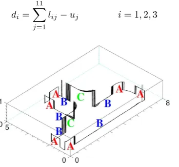
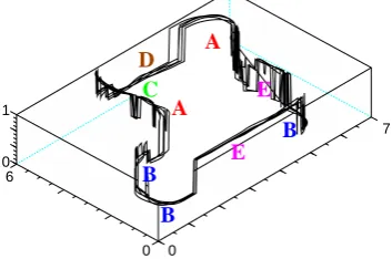
The second experiment is more complex than the first one. Here, the robot has to follow a particular route in a more complex environment, where the causal relationship between the sensory perception of the robot and the mo-tor responses varies along the trajecmo-tory (Figure 6). As in the previous experiment, first the programmer drives the robot manually using a joystick to demonstrate the desired route to the robot and during this run, laser perception of the robot (u₁−u11) and the desired motor responses were

Fig. 6. Experiment 2. The desired route for the robot to learn. The programmer drives the robot manually, using a joystick to demonstrate the desired route to the robot

Having obtained the training data set, we used the K -means algorithm to divide the perception space of the robot into five clusters,A,B,C,DandE.

Figure 7 shows the graphical illustration of these five centroids.

laser index magnitude

A

B

C

E

D

(m)

1 2 3 4 5 6 7 8 9 10 11 0.5

1.2

1.0

Fig. 7.Experiment 2. Graphical illustration of each centroid.

The internal map of the robot along the desired route which shows how the sensory data is clustered into 5 classes is illustrated in Figure 8.

6

0 0

7

0 1

B

B B

D

E E A

A

C

Fig. 8. Experiment 2. The internal map of the robot which clusters the environment into5different regions.

Once we had classified the sensory perception of the robot into distinctive classes, we then obtained one AR-MAX model for each cluster, which links the laser readings (u₁−u11) of the robot to the desired angular velocity (ω)

(to simplify the experiments, we clamped the linear veloc-ity of the robot at 0.15 m/s). The models for each cluster

A,B,C,DandEare given in Tables 2 and 3 respectively. These tables also present the error reduction ratio (ERR)

value of each term presented in the polynomial, where the ERR values provide an indication of the contribution that each term in the model makes to the desired output vari-ance.

Region A Region B Region C

ERR ω_A= ERR ω_{B =} ERR ω_C=

0.00 −0.053 0.00 −0.477 0.00 +1.208

1._{27 −0}._048·u1(n) 4.34 ₋0.533_·u1(n) 21.12₋0.436_·u1(n)

0.84 −0.051·u2(n) 1.50 +0.053_·u2(n) 1.38 ₋0.028_·u2(n)

0._{26 +0}._057·u3(n) 0.73 +0.027_·u3(n) 4.66 +0.708_·u3(n)

1.00 −0.064·u4(n) 3.18 −0.318·u4(n) 14.79−0.500·u4(n)

0.42 −0.029·u5(n) 0.13 +0.155_·u5(n) 1.65 ₋0.048_·u5(n)

30.₉₈₋₀._487·u6(n) 34.54 +0.399_·u6(n) 0.00 +0.000_·u6(n)

1.03 +0.595·u7(n) 8.94 +0.077_·u7(n) 0.26 +0.046_·u7(n)

3._{42 +0}._148·u8(n) 3.34 +0.264_·u8(n) 0.60 ₋0.110_·u8(n)

0.00 +0.000·u9(n) 0.39 +0.135_·u9(n) 0.26 +0.046_·u9(n)

0._{38 +0}._028·u10(n) 0.71 ₋0.100_·u10(n) 13.24₋0.886_·u10(n)

4._{41 −0}._145·u11(n) 4.60 +0.264·u11(n) 0.08 −0.091·u11(n)

Table 2

Experiment 2. The polynomial ARMAX models which relate the laser readings of the robot (u1 tou11) to the angular

velocity (ω_{) in regions}A_,B_andC_{respectively.}

Region D Region E

ERR ωD= ERR ωE=

0._{00 +7}._{443 0}._{00 −2}.₆₁₂

5.04 −0.040·u1(n) 5.10 +0.006_·u1(n)

12._{27 +0}._652·u2(n) 0.59 +0.503_·u2(n)

0._{46 −1}._029·u3(n) 16.14 +0.459·u3(n)

0.00 +0.000·u4(n) 0.15 ₋0.059_·u4(n)

0._{00 +0}._000·u5(n) 3.09 +0.001_·u5(n)

3.85 −0.052·u6(n) 1.37 +1.080_·u6(n)

21.₉₁₋₂._293·u7(n) 0.88 +0.063_·u7(n)

1._{68 −3}._967·u8(n) 5.62 +0.102·u8(n)

2.42 +0.373·u9(n) 8.68 +1.012_·u9(n)

0._{21 +0}._112·u10(n) 1.14 +0.542_·u10(n)

1.23 −0.190·u11(n) 3.18 ₋0.583_·u11(n)

Table 3

Experiment 2. The polynomial ARMAX models which relate the laser readings of the robot (u1 tou11) to the angular

velocity (ω) in regionsDandE.

correct polynomial obtained specifically for that region to drive the robot. Once the robot reaches the next region, the second polynomial is activated and the procedure goes on in this way.

The results show that the robot was successfull following the desired route without losing the track or crashing into obstacles. Note that when we tried to model the sensor-motor relationship with asinglepolynomial — rather than dividing the environment into subregions and obtaining one polynomial for each region — the resultant model failed to drive the robot successfully along the desired route.

Fig. 9.Experiment 2. The trajectory of the robot under the control of the polynomial ARMAX models given in Tables 2 and 3.

3. Modelling Complex Robot Training Tasks through Bootstrapping System Identification

In the previous section we discussed that it is important to have information about the present state of the robot to determine the robot’s next action. We therefore introduced a novel code generation method based on first recognizing distinctive landmarks in the environment, using unsuper-vised clustering algorithms, and then generating a different sensor-motor model for each landmark, using system iden-tification.

However, it is possible that for some of these landmarks, the desired task is still too complex to be modelled with a di-rect link between raw sensory data and the motor response of the robot. In these cases it is common that the raw input readings are preprocessed with the aid of the programmer to extract higher level information from the sensory data in order to simplify the problem even further. However, pre-processing makes the code-generation process programmer-dependent, and as it is a manual, non-deterministic pro-cess, may result in suboptimal models.

We argue that it is important to have a formal, algorith-micmethod to extract high level input information, mini-mizing the use of human knowledge. We therefore propose a bootstrapping behaviour generation method which uses low level behaviours and the information about the cur-rent state of the robot to generate more complex ones. The method has three phases:

Phase 1 For obtaining simple sensor-motor controllers, we use the main modelling approach given in Section 1. Some examples of such low level reactive-controllers are obstacle-avoidance, door traversal, wall-following, etc.

Phase 2 The controllers obtained in phase 1 are loaded into the robot in order to form a behaviour repertoire in the robot’s memory. We then obtain a NARMAX model, which models the new task as a function of these previously acquired behaviours. Here, the selection of behaviours is done using state variables which contain information about the state of the environment and the robot (see Figure 10).

Behaviour Repertoire

Variables State Perception

Sensor

Raw Polynomial NARMAX

Model

Motor Response

Fig. 10. The bootstrapping method of generating complex robot training tasks.

Phase 3 Once we have obtained the NARMAX model, we test it on the robot in order to validate its performance. If the new controller is successful it is added to the reper-toire so that it can be used to generate even higher level controllers in the future.

The viability of the proposed method is demonstrated by a set of real robot experiments where aScitos G5 mo-bile robot was trained methodically to accomplish various sensor-motor tasks starting from simple obstacle avoidance to complex route learning.

3.1. Experiment 3. Modelling Advanced Obstacle Avoidance Behaviour

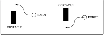
In the third experiment, we trained the robot to avoid obstacles towards the “obvious” side, as shown in Figure 11; if robot has more space on the right side, it turns to right, and if there is more space on the left, it turns to left.

OBSTACLE

ROBOT

OBSTACLE

ROBOT

Fig. 11. Experiment 3. The desired obstacle avoidance be-haviour.

16 times. During each run, laser readings and the motor commands of the robot were logged in every 250 ms.

Fig. 12.Experiment 3. The trajectory of the robot, guided by the programmer. The robot was started from point S and avoided boxes along the route until it reached the destina-tion point F.

Having obtained the training data, we coarse-coded laser readings into 11 sectors by averaging 62 readings for each 22◦ _{interval. Coarse-coded laser readings were clipped at}

1.5 m to avoid models taking far-away obstacles into ac-count, as these irrelevant to obstacle avoidance.

We then modelled the angular velocityωoof the robot as

a function of coarse-coded laser readings (u₁−u11) using

ARMAX system identification. The obtained model was a linear polynomial with 6 terms (Table 4).

ω₍n_{) = +0}.₁₈₃₋₀._187·u4(n)₋0.137_·u5(n)

−0.021·u6(n)₋0.045_·u7(n) + 0.265_·u8(n)

Table 4

Experiment 3. The ARMAX model which links the laser per-ception to the angular velocity of the robot to achieve ad-vanced obstacle avoidance behaviour.

Model Validation We tested the steering speed model on the robot in three different test environments. During the experiments the linear speed of the robot was clamped to 0.1 m/s.

In the first test environment, the robot was started from 20 different initial positions in front of two boxes put next to each other and was expected to avoid them towards the “obvious” side. The results (Figure 13 show that the robot was able to avoid obstacles as desired1_.

In the second (Figure 13b) and third (Figure 13c) test en-vironments, we tested if the obtained angular speed model captured the real essence of obstacle avoidance behaviour. The robot was started in front of the boxes arranged to sim-ulate a right and a left corner and in both cases the robot was successfull in avoiding the corners by turning the “ob-vious” side. Note that for both environment the robot was started from 16 different initial positions.

1

In three runs out of 20 the robot was not able to choose a side and failed to escape from the boxes (visible in figure 13a). A possible solution to this problem would be to train a linear speed model as well.

(a) (b) (c)

Fig. 13.Experiment 3. The three environments where the ob-tained angular speed model ωo given in table 4 was tested

for obstacle avoidance behaviour.

3.2. Experiment 4: Obstacle Avoidance based on Object Colour

In a fourth experiment, we trained the robot in such a way that it determined the turning direction according to the colour of the obstacle, rather than choosing the “obvious” side: while the robot approaches an obstacle, it identifies the colour of the obstacle, and avoids red obstacles by a right turn, green obstacles by a left turn.

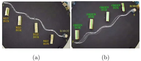
To obtain the training data set, we drove the robot in two environments. The first one contained boxes of red colour, resulting in right-turn obstacle avoidance (Figure 14a), the second environment contained green boxes, resulting in left-turn obstacle avoidance (Figure 14b). In each environment, we conducted the experiments 10 times starting the robot from initial point S, stopping at the final point F.

(a) (b)

Fig. 14.Experiment 4. The trajectories of the robot in two training environments. The first one, shown on the left, con-tained boxes of red colour, resulting in right-turn obstacle avoidance, the second environment, shown on the right, con-tained green boxes, resulting in left-turn obstacle avoidance.

During the experiments, we logged the coarse-coded laser readings and the motor responses of the robot as well as the colour indexci (ci = 1 for green,ci= 2 for red boxes)

of the closest obstacle to the robot every 250 ms.

After logging this perception-action data, we modelled the angular speedωtof the robot as a function of the

coarse-coded laser readings (u₁−u11) and the colour index of the

detected obstacle (ci), using NARMAX system

identifica-tion. The NARMAX model contained 21 terms (Table 5). The resultant polynomial modelωtis essentially the

com-bination of two polynomials, where each polynomial turns the robot to a different direction, and the transition be-tween the two is performed using the terms including state variableci(the last two rows in Table 5).

ωt(n) = +3.839−0.661·u4(n)₋0.212_·u5(n)

+0._650·u7(n)₋2.413_·u8(n)₋0.093_·u4(n)2

+0._150·u5(n)2₋0.002_·u7(n)2+ 0.050_·u8(n)2

−0.202·u4(n)_·u5(n)₋0.098_·u4(n)_·u6(n)

−0.546·u4(n)_·u7(n) + 1.121_·u4(n)_·u8(n)

−0.249·u5(n)_·u6(n) + 0.076_·u5(n)_·u7(n)

−0.129·u6(n)_·u7(n) + 0.130_·u6(n)_·u8(n)

−1.469·ci(n) + 0.263·ci(n)·u5(n)

+0.369·ci(n)·u6(n) + 0.280_·ci(n)∗u7(n)

Table 5

Experiment 4. The NARMAX model for the angular speed of the robot for colour-encoded obstacle avoidance.

Model Validation As before we validated the performance of the obtained angular speed model by testing it on the robot. We put the robot in front of red and green boxes and let the model drive the robot. For each coloured box, the model was tested 16 times and the resultant trajectories of the robot are given in Figure 15. They confirm that the model given in Table 5 achieves the desired behaviour.

(a) (b)

Fig. 15.Experiment 4. The resultant trajectories of the robot guided by the angular speed modelωtgiven in Table 4 when

it is confronting the: (a) red coloured boxes and (b) green coloured boxes.

In order to quantify the performance of the angular speed modelωt, we computed the strength of the association

be-tween the colour of the detected obstacle and the direc-tion of the corresponding turning speed of the robot using

Cramer’s Vtest. To do so, we checked the sign of the resul-tant turning speed according to the colour of the detected obstacle during the test runs. When the robot detected a green obstacle, the resultantωt>0 (indicating to turn left)

97.651% of the time, and when the detected obstacle is red,

ωt<0 (indicating to turn right) 98.837% of the time. The

results showed that there is a significant correlation (V = 0.96, note thatV varies between 0 and 1, corresponding to “no association” and “perfect association” respectively). 3.3. Experiment 5. Colour Encoded Route Learning Behaviour

The previous experiment demonstrates how different be-haviours can be embodied in a single polynomial where the transition between behaviours is done using state variables

containing information about the current state of the envi-ronment. We will now show that this can be used to achieve more complex tasks.

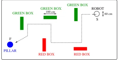
Scaling up from the 3rd and 4th experiment, the fifth task was to generate a polynomial which can guide the robot to follow a particular route in order to reach a desired object. The experimental scenario is given in Figure 16, the environment is populated with red and green boxes in order to guide the robot to the destination pointF, where the target object, a blue pillar, is present.

60 cm 100 cm

ROBOT

PILLAR

RED BOX GREEN BOX GREEN BOX

RED BOX GREEN BOX

F

S

Fig. 16.Experiment 5. The experimental scenario where the desired task is to teach the robot to follow a particular route in order to reach the blue pillar at point F.

To collect the training data, the programmer drove the robot manually in the target environment (Figure 17) 10 times starting the robot from the initial position S and stopping the robot in front of the blue pillar (destination pointF). During the training, laser readings, camera im-ages and the motor commands of the robot were logged in every 250 ms.

Fig. 17.Experiment 5. The trajectories of the robot guided manually by the human operator in order to obtain the train-ing data.

Bootstrapping from Low-Level Controllers After logging the training data we processed the laser readings and the raw images to extract three low level controllers which were then be fed to the polynomial NARMAX models as inputs. These controllers are:

(i) Obstacle avoidance controllerThe first controller in the behaviour repertoire guides the robot to avoid obstacles. Here we used the polynomial model ωo

(ii) Colour encoded turning controller The second behaviour turns the robot to the right if the colour of the detected object is red, and to the left if the colour is green. Here we used the polynomial modelωtgiven

in table 5, obtained during experiment 4.

(iii) Object seeking controllerWe also implemented a simple object seeking controller which looks for the nearest object in front of the robot and guides the robot towards it.

Having identified the controllers, we also obtained three state variables which will help the system identification pro-cess to link the low level controllers to achieve the desired task:

(i) didefines if the target object is detected or not;d= 0

represents target object is not detected, and di = 1

represents target object is detected.

(ii) oi defines if there is an obstacle close to the robot;

oi = 0 represents there is no obstacle detected, and

oi= 1 represents the presence of an obstacle.

(iii) ci states the colour of the detected obstacle; ci = 1

represents green, ci = 2 represents red, and ci = 0

represents all other colours.

We then obtained two polynomial models; one for the linear speed vr and one for the angular speed ωr of the

robot — as a function of the predefined behaviours (ωo,ωt

andωw) and the state variables (di,oiandci) (Figure 18).

The obtained models are given in Table 6.

ω

ci

oi di

]

ω

ω

ω

]

[

[

NARMAX model

Fig. 18.Experiment 5. The bootstrapping method of generat-ing complex route learngenerat-ing behaviour usgenerat-ing predefined low level controllers; obstacle avoidance (ωo), left/right

turn-ing (ωt) and object seeking (ωw). In order to link the

be-haviours we also present three state variables indicating the presence of the target object (di), presence of the obstacles

(oi) and the colour of the detected obstacles (ci).

vr(n) = +0.100₋0.100_·di(n)

ωr(n) = +0.100·d(n) + 1.000·ωw(n)

−1.000·oi(n)·ωw(n) + 1.000·oi(n)·ωo(n)

−1.000·oi(n)·ci(n)·ωo(n) + 1.000·oi(n)·ci(n)·ωt(n)

+1._000·di(n)·oi(n)·ωw(n)−1.000·di(n)·oi(n)·ωo(n)

+1._000·di(n)·oi(n)·ci(n)·ωo(n)

−1.000·di(n)·oi(n)·ci(n)·ωt(n)

Table 6

Experiment 5. The polynomial models for the linear vr and

angular speedωr of the robot.

3.3.0.1. Model Validation Having obtained the percep-tion modelsvr and ωr, we tested them on the robot. We

let the models drive the robot in the target environment 10 times. Figure 19 shows the resultant trajectories, where in each run the robot was successful to reach the target object.

Fig. 19. Experiment 5. The trajectories of the robot under the control of the perception models given in Table 6.

3.4. Extended Bootsrapping Method

In experiment 3 we demonstrated how simple NARMAX models can be used to achieve more complex tasks. One interesting question here is “what happens if the low level controllers found in the behaviour repertoire are not ade-quate to generate the desired task?”

To address this question, we extended the proposed method by adding raw sensory perception to the modelling process. In this way, we let the polynomial model combine raw sensory data with the low-level controllers automat-ically. Again, the transition between the controllers and the raw sensory data is controlled according to the state of the environment and the robot (Figure 20).

Behaviour Repertoire

Perception Sensor

Raw

Model NARMAX Polynomial

Variables State

Motor Response

Fig. 20. The extended bootstrapping method of generating complex robot training tasks. In the extended version we also give raw sensory data as inputs to the system.

3.5. Experiment 6. Complex Route Following combined with Door Traversal Behaviour

pillar, it has to wait with zero linear and angular speeds until the pillar is removed from the environment (stage 2). Once the pillar is removed, the robot must complete the route by traversing the two consecutive door-like openings to reach the destination point F.

GREEN BOX

RED BOX PILLAR

1m

1m

2m 2m

ROBOT

S

F

W BOX

BOX

BOX BOX

Fig. 21.Experiment 6. The experimental scenario for the de-sired complex route learning task.

As before we obtained the training data by driving the robot manually in the target environment shown in Fig-ure 22. Starting the robot at initial position S, first we drove the robot to point W. Then the robot was stopped in front of the pillar until the pillar was removed by the human oper-ator. We then continued driving the robot to pass through two consecutive door-like openings. The experiments were repeated 10 times and for each run we logged the laser per-ception, camera images and the motor commands of the robot in every 250 ms.

Fig. 22. Experiment 6. The trajectories of the robot under the manual control of the human operator for training data collection.

Obtaining Sensor Based Models After logging the training data, we fed the raw perception data to low-level controllers present in the behaviour repertoire of the robot to generate higher level inputs for the desired task. But this time we also coarse-coded the laser readings into 11 sectors (u₁−u11)

by averaging 62 readings for each 22◦_{in order to enrich the}

system inputs, since there is no dedicated door traversing controller in the behaviour repertoire of the robot. Also for the transition between the behaviours, we computed a state flagsiwhich indicates if the blue pillar is removed from the

front of the robot (si= 1) or not (si= 0).

We then obtained two NARMAX models, expressing

vc and ωc as a function of coarse-coded laser readings

(u₁. . . u₁₁), route following controllersvrandωrobtained

in Section 3.3, and state variablesi. The obtained models

are given in Table 7.

vc(n) = +vr+ 0.1·si(n)

ωc(n) =−0.033 + 1.016·ωr(n) + 0.144·u4(n)

−0.088·u5(n) + 0.004_·u6(n)₋0.131_·u7(n)

+0._014·u8(n) + 0.208_·ωr2(n)−0.026·u24(n)

+0.029·u25(n) + 0.062·u 2 7(n)

2

−0.025·u4(n)_·u8(n)

+0.394·si(n)−1.051·si(n)·ωr(n)

−0.145·si(n)·u4(n)₋0.060_·si(n)·u5(n)

−0.040·si(n)·u6(n) + 0.026_·si(n)·u7(n)

Table 7

Experiment 6. The polynomial models for the linear and angu-lar speed of the robot for complex route learning and door traversal behaviour. The last three rows show the terms in-cluding state variablesi.

Model Analysis and Validation Once we obtained the sen-sor based models, we used them drive the robot in the tar-get environment in order to validate the performance. Fig-ure 23 shows the trajectories of the robot for 10 runs, where the robot completed the track successfully in each attempt.

Fig. 23.Experiment 6. The trajectory of the robot under the control of the perception models given in Table 7.

Transparent Models Having transparent models like the ones given in Table 7 has a number of advantages, for exam-ple the possibility to analyse the robot behaviour formally. Here, for instance, one can see that the model of Table 7

ωc has two components. The first one is the colour-based

route following behaviour which was previously obtained in section 3.3, taking the control of the robot when state flagsi equals 0. The second behaviour is a door traversal

controller activated whensi = 1.

4. Conclusion

This paper demonstrates, in theory and practical robotics experiments, how system identification can be used to generate complex robot training tasks, i.e. tasks that are context-dependent, and require memory for successful completion. Those tasks cannot normally represented by a single model, and we show how several models can be combined into one by a simple bootstrapping method.

In Section 2, we emphasize the importance of detecting these transitions and propose a novel method to estimate them. The method relates distinctive locations in the en-vironment to the state of the robot, using an unsupervised clustering algorithm.

Once we estimate the current state of the robot accu-rately, the next step is to combine this state information with the perception of the robot to generate the essential motor commands, to accomplish the desired complex robot training tasks. One way of addressing this issue is to gener-ate a separgener-ate sensor-motor couplings for each stgener-ate of the robot. The viability of this method has been demonstrated by modelling right wall following and complex route learn-ing behaviours.

However there are cases where for some of these land-marks, the desired task is still too complex to be modelled with a direct link between raw sensory data and the mo-tor response of the robot. Therefore, in Section 3, we intro-duce a bootstrapping method of generating complex robot training tasks using polynomial NARMAX structures. The method is based on obtaining hierarchical polynomial mod-els which model the desired task by combining predefined low level sensor motor controllers and raw sensory data.

This allows us to combine different low level controllers in a single polynomial to achieve more complex tasks. The transition between these controllers is done using state vari-ables which contain information about the state of the en-vironment. To demonstrate the viability of the proposed method, we generated a complex route following polyno-mial which computes the desired motor responses of the robot based on the inputs from low level controllers (such as obstacle avoidance and colour encoded turning controllers). The method also allows as to combine the raw sensory data of the robot with the previously defined low level trollers. This does not only produce robust high level con-trollers to achieve the desired task, but also enables us to extract new low-level controllers from the generated con-troller. The obtained polynomial model for the complex route learning behaviour includes a door traversal con-troller generated automatically using raw sensory data for the second part of the desired route.

Future Work In Section 2, we estimate the the state of the robot based on its current sensory perception assuming that state information is observable through robot sensors. However there are cases where multiple states are indis-tinguishable to the robot because of the perceptual

simi-larities (perceptual aliasing [26]).

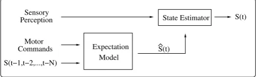
In these kind of situations, state estimation can not be based on only the current sensory perception of the robot, but some extra information is needed. One way of dealing with the perceptual aliasing problem is to incorporate an expectation model — a model which estimates the next state of the robot based on the previous states and the ac-tions of the robot — into the recognition of locaac-tions (Fig-ure 24). With the incorporation of the expectation model, the robot would have a rough idea about which state it is going to and would be able to combine this information with its current sensory readings to estimate the next state accurately. Therefore we are currently investigating ways of developing a formal method to obtain expectation models automatically and incorporating them into the state esti-mation process.

State Estimator Sensory

Perception

S(t)

S(t)

Commands Motor

Model Expectation

S(t−1,t−2,...,t−N)

Fig. 24.The incorporation of the expectation model to the process of estimating the current state of the robot. The expectation model predicts the next stateSˆ₍t_{)of the robot,} based on the previous states and the actions of the robot. The state estimation model then combines the current sensory readings of the robot with the expected state information to predict the next stateS(t)of the robot.

Furthermore we are working on the integration of the state estimation process with robot training and the NAR-MAX system identification methods in a single framework in order to develop a formal method of generating com-plex robot training tasks automatically and algorithmically without needing explicit knowledge of robot programming. The work already carried out and that proposed forms part of our ongoing research in universities of Ulster, Essex and Sheffield.

Acknowledgments

We express our thanks to Emre ¨Ozbilge for his contribu-tion to the experimental work presented in this paper.

References

[1] U. Nehmzow,Mobile Robotics: A practical introduction, 2nd ed. Springer Verlag, 2003.

[2] ——, “Quantitative analysis of robot-environment interaction – towards “scientific mobile robotics”,” International Journal of Robotics and Autonomous Systems, vol. 44, pp. 55–68, 2003. [3] U. Nehmzow and K. Walker, “The behaviour of mobile robot is

chaotic,”AISB Journal, vol. 1(4), pp. 373–388, 2003.

[4] T. Kyriacou, U. Nehmzow, R. Iglesias, and S. A. Billings, “Task characterization and cross-platform programming through system identification.” International Journal of Advanced Robotic Systems, vol. 2, pp. 317–324, 2005.

[5] R. Iglesias, T. Kyriacou, U. Nehmzow, and S. Billings, “Robot programming through a combination of manual training and system identification,” in Proc. of ECMR 05 - European Conference on Mobile Robots 2005. Springer Verlag, 2005. [6] U. Nehmzow, O. Akanyeti, C. Weinrich, T. Kyriacou, and

S. Billings, “Robot programming by demonstration through system identification,” inIROS, San Diego, USA, 2007. [7] O. Akanyeti, U. Nehmzow, C. Weinrich, T. Kyriacou, and

S. Billings, “Programming mobile robots by demonstration through system identification,” in ECMR, Freiburg, Germany, 2007.

[8] S. Lauria, G. Bugmann, T. Kyriacou, J. Bos, and E. Klein, “Training personal robots using natural language instruction,”

IEEE Intelligent System, vol. 16, pp. 38–45, 2001.

[9] A. Dearden and Y. Demiris, “Learning forward models for robots,” inProceedings of the International Joint Conference on Artificial Intelligence, Edinburgh, UK, 2005, pp. 1440–1445. [10] A. Billard and G. Hayes, “Learning to communicate through

imitation in autonomous robots,” in In 7th International Conference on Artificial Neural Networks. Springer-Verlag, 1997, pp. 763–768.

[11] O. Akanyeti, U. Nehmzow, and S. Billings, “Robot training using system identification,” Int. J. Robotics and Autonomous Systems, 2008, (in press).

[12] R. Iglesias, U. Nehmzow, and S. Billings, “Model identification and analysis in robot training,” in Proc. of TAROS 2007, (Towards Autonomous Robotic Systems). Springer Verlag, 2007, pp. 40–47.

[13] P. Eykhoff, System Identification: parameter and state estimation. London: Wiley-Interscience, 1974.

[14] ——,Trends and Progress in System Identification. Pergamon Press, 1981.

[15] S. Chen and S. Billings, “Representations of non-linear systems: The narmax model,”International Journal of Control, vol. 49, pp. 1013–1032, 1989.

[16] S. Billings and S. Chen, “The determination of multivariable nonlinear models for dynamical systems,” in Neural Network Systems, Techniques and Applications, C. Leonides, Ed. Academic press, 1998, pp. 231–278.

[17] I. Sobol, “Sensitivity estimates for nonlinear mathematical models,” Mathematical Modelling and Computational Experiments (MMCE), vol. 1, pp. 407–414, 1993. [18] K. Chan, A. Saltelli, and S. Tarantola, “Sensitivity analysis of model output: Variance-based methods make the difference,” in Proc. of 1997 Winter Simulation Conference, (Towards Autonomous Robotic Systems), 1997, pp. 261–268.

[19] R. Iglesias, U. Nehmzow, T. Kyriacou, and S. Billings, “Modelling and characterization of a mobile robot’s operation,” inCAEPIA 2005, 11th conference of the Spanish association for Artificial Intelligence, Santiago de Compostela, Spain, 2005. [20] A. Saltelli, K. Chan, and E. M. Scott, Sensitivity analysis.

Wiley, 2000.

[21] U. Nehmzow, O. Akanyeti, and S. Billings, “A proposal of a methodology for the analysis of robot-environment interaction

through system identification,” inTAROS, Edinburgh, Scotland, 2008.

[22] U. Nehmzow,Robot Behaviour — Design, Description, Analysis and Modelling. Heidelberg, New York, London: Springer, 2009. [23] O. Akanyeti, T. Kyriacou, U. Nehmzow, R. Iglesias, and S. Billings, “Visual task identification and characterization using polynomial models,”Int. J. Robotics and Autonomous Systems, vol. 55, pp. 711–719, 2007.

[24] H. I. Christensen, “Slam paper repository,” 2005. [Online]. Available: http://www.cas.kth.se/SLAM/slam-papers.html [25] J. B. MacQueen, “Some methods for classification and

analysis of multivariate observations,” in Proc. of 5-th Berkeley Symposium on Ma5-thematical Statistics and Probability, Berkeley, USA, 1967, pp. 281–297.