promoting access to White Rose research papers
White Rose Research Online
Universities of Leeds, Sheffield and York
http://eprints.whiterose.ac.uk/
This is an author produced version of a paper accepted for publication in Journal of Intelligent Material Systems and Structures.
White Rose Research Online URL for this paper: http://eprints.whiterose.ac.uk/8881/
Published paper
Batterbee, D. and Sims, N.D. (2009) Temperature sensitive controller
performance of MR dampers. Journal of Intelligent Material Systems and
Structures, 20 (3). pp. 297-309.
http://dx.doi.org/10.1177/1045389X08093824
Batterbee, D., and Sims, N. D. (2009). "Temperature Sensitive Controller Performance of MR
1
INTRODUCTION
It is well known that smart fluids (electrorheological (ER) and magnetorheological (MR))
provide an effective means to implement semi-active vibration control. This is achieved
through alteration of the fluid’s yield stress on the application of an electric or magnetic field.
MR based devices have received particular commercial success for over a decade, and recent
examples include the suspension systems featured on the 2007 Ferrari 599 GTB Fiorano
(Delphi Press Release, 2006b), and the 2007 Audi TT (Delphi Press Release, 2006a). One
aspect of the design that has received relatively little attention is related to the effects of
temperature. Changes in temperature will alter the smart fluid’s properties, but control
systems are often designed without due consideration of this fact. The highly non-linear
behaviour of smart fluid dampers has also meant that there is still little consensus on how to
best perform control. The present study aims to address these issues.
Smart fluid dampers exhibit temperature changes due to the heating associated with energy
dissipation. This effect will be particularly significant in a continuously excited system such
as a vehicle suspension. Choi, et al. (2005) noted that in a passenger vehicle, ER dampers
could reach temperatures of up to 100°C. Harsh operating environments will also have an
influence: In aircraft or building applications there will be large temperature variations.
Previous work has to a certain degree illustrated the effects of temperature on smart fluid
dampers. Gordaninejad and Breese (1999) presented experimental results on different sized
MR dampers, and illustrated significant reductions in peak force with rising temperature.
This was attributed to the reduced viscosity of the fluid, although the authors did not consider
control system effects. The work was later extended to show how fins can be used to
augment heat transfer and minimise the rise in temperature (Dogruoz et al., 2003). Choi, et
an increase with rising temperature. The data was used to construct a quasi-steady
temperature dependant model of an ER damper, and subsequently included within a quarter
car simulation. Sliding mode control was shown to be effective at two temperatures. Liu, et
al. (2003) developed a temperature dependant skyhook controller for an MR vehicle
suspension. Using a quasi-steady damper model, simulations were performed to show how
temperature feedback can improve performance by adjusting the controller for variations in
viscosity.
In light of the above it is clear there are some limitations in the work related to temperature
effects in smart fluid dampers. More specifically:
• Previous work has only considered the variation of a single fluid property with
temperature e.g. viscosity or yield stress. In practice, all of the fluid properties could be
affected and impact on control system performance.
• Investigations are usually based on quasi-steady damper models. Temperature
dependant dynamic affects, e.g. fluid compressibility, are likely to be important.
• Control studies have been based on numerical modelling, and have not been validated
experimentally. Furthermore, different control strategies have not been compared.
The present contribution aims to address the above issues through a numerical and
experimental investigation of an MR vibration isolator subject to temperature variation. The
paper is organised as follows. First, an experimental facility used to perform MR damper
tests at different temperatures is described. Experimental data is then used to identify the MR
damper’s fluid properties as a function of temperature. Next, a temperature dependant MR
damper model that accounts for dynamic effects is developed and experimentally validated.
single-degree-of-freedom (SDOF) mass isolator is used as a case study and experiments are performed using
the hardware-in-the-loop-simulation (HILS) method. Various control strategies are
investigated in order to assess their relative performance and robustness against temperature
uncertainty. Using the temperature dependant MR damper model, simulations are also
performed to help explain the observed behaviour.
2
DESCRIPTION OF THE DAMPER TEST FACILITY
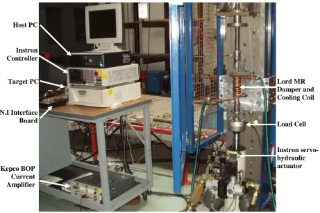
A photograph of the experimental setup is shown in Figure 1. This comprised an Instron
servo-hydraulic actuator (Instron Structural Testing Systems, 2007), which was used to excite
Lord Corporation’s RD-1005 MR damper (Lord Corporation, 2007). The actuator was rated
at ±25kN, ±50mm and ±1ms-1, and included a built-in inductive displacement transducer and dynamic load cell. The MR damper is shown schematically in Figure 2. Here, fluid flows
through an annular orifice, and the magnetic field is generated via a coil wrapped around a
steel bobbin. An accumulator is also included to accommodate for the change in working
volume as the piston rod displaces. Current was supplied to the damper using a Kepco BOP
amplifier (Kepco Inc., 2007), which was used in current control mode. This ensured that the
magnetic field was independent of temperature, despite changes in the coil’s resistance. To
cool the damper after testing at high temperatures, copper tubing was wrapped around the
body and fed with cold water (see Figure 1). This also dictated the minimum temperature for
the damper tests (≈11°C). The temperature was measured using a thermocouple positioned at
the centre of the damper’s body. The thermocouple was insulated from the surrounding
copper tubing in order to prevent inaccurate temperature measurements. To increase the MR
damper’s temperature, successive 5mm-4Hz sine wave cycles were applied and the current
was set to 0.25A. Once the desired temperature was reached, the data from a particular test
by the maximum safe operating value for the device. Data acquisition was achieved using a
National Instruments PCI-MIO-16XE-10 card.
3
TEMPERATURE SENSITIVE MR DAMPER BEHAVIOUR AND
MODELLING
Some typical experimental force/velocity and force/displacement responses for temperatures
in the range of 14-71°C are shown in Figure 3. The data corresponds to a 10mm, 8Hz
sinusoidal excitation and the current was set to 1A. Clearly, there is a significant change in
the MR damper’s behaviour, and this could have major implications on the performance of a
control system.
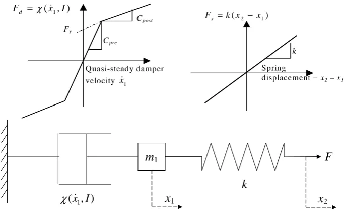
A numerical model can help us better understand the behaviour shown in Figure 3. One
modelling format, which has been developed and investigated extensively by the present
authors (Batterbee and Sims, 2005, Sims et al., 2004), is illustrated in Figure 4. Here, a
bi-viscous damper is connected in series with a mass and a linear spring. This is a reasonably
straightforward model in comparison to other frequently adopted modelling formats, for
example Bouc-Wen (Spencer Jr. et al., 1997). However, the model can be strongly linked to
the constitutive behaviour of the device, which makes it highly suitable for understanding the
effects of temperature. For example, the valve flow (which is assumed to be quasi-steady) is
represented by the non-linear function χ and is a function of the quasi-steady velocity x&1 and
the control signal I to the smart damper. This non-linear function contains information about
the MR damper’s yield force Fy and the fluid’s viscosity, which has two parts – a linear
pre-yield viscosity Cpre and a linear post-yield viscosity Cpost. Thedamper stiffness k accounts for
fluid and accumulator compressibility and this dictates the size of the hysteresis loop in the
force/velocity response. This damper stiffness term will be influenced by the fluid’s bulk
lumped mass m1 represents fluid inertia and gives rise to the oscillations when the piston
velocity changes direction. This maintained a constant value equal to 2kg, which was shown
to correlate well in previous work (Sims et al., 2004). Finally, the co-ordinate x2 corresponds
to the displacement of the damper piston.
With the help of this model description, the three key effects of rising temperature on the
response shown in Figure 3 can be described as follows:
• There is a reduction in the yield force Fy, which corresponds to a reduction in the MR
fluid’s yield stress.
• The slope of the post-yield force/velocity response decreases (see Figure 3(a)), which
is associated with a reduction in the fluid’s viscosity.
• The size of the hysteresis loop in the force/velocity response reduces. This is
associated with a change in the damper’s stiffness caused by the rising accumulator
pressure. The effect can also be observed in the force/displacement response when the
damper changes direction. As shown in Figure 3(b), the slope of the
force/displacement curve increases with temperature in this region.
Through more careful observation of Figure 3, it can also be seen that the offset in the
response slightly increases with temperature due to the rising gas accumulator pressure. This
is best observed in Figure 3(a) by noting that the difference in the force at minimum velocity
is greater than that at maximum velocity. The model given in Figure 4 does not account for
this static gas spring force. Nonetheless, it has generally been found that this accumulator
offset has an insignificant effect on the performance of MR suspension systems. This is
because the parallel stiffness of the accumulator is usually insignificant in comparison to the
statement holds and thus the effect of the accumulator offset was neglected in the numerical
modelling in this paper.
The next stage is to identify the model’s parameters and to establish their relationship as a
function of temperature. Sims et al. (2004) described a formal approach for identifying the
parameters of the model shown in Figure 4. A more straightforward approach was adopted in
the present study, and for each stage in the identification process, the most appropriate
excitation condition was chosen for the parameter under consideration. It will later be
important to validate the model against a range of excitation conditions. For simplification
purposes, the pre-yield viscosity Cpre was assumed to be independent of temperature. This
maintained a constant value equal to 100kNsm-1, which was found to be accurate in previous work (Sims et al., 2004). The post-yield viscosity Cpost was determined as the slope of the
MR damper’s force/velocity response after yield. Only decelerating data was used in order to
remove the effects of fluid inertia, and a 10mm-8Hz sine wave was chosen as the input
excitation to identify the variable. This velocity amplitude (0.5ms-1) approximately corresponded to the range observed in the controlled suspension system investigations
(Section 4). Furthermore, the relatively high velocity excitation maximised the number of
data points in the post-yield region thus improving the accuracy of the identification. The
yield force Fy was calculated by taking the intercept of a straight line fit to the decelerating
post-yield force/velocity data. The accumulator offset in the force/velocity data was also
removed such that the resulting yield forces in the compression and extension phases were
approximately equal. As yield force is a parameter defined at zero velocity, a lower velocity
5mm-4Hz input excitation was used for the identification. The chosen input also minimised
the dynamic effects in the yield region (i.e. at low velocities), thus improving the validity of
the calculation. Finally, the damper stiffness term k was identified by fitting a straight line to
direction. Higher current data was used as this amplifies the compressibility effect, and
provides a better correlation with the experimental data.
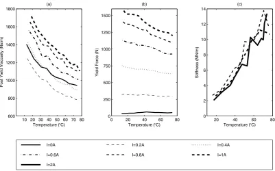
The identified parameters are shown as a function of temperature in Figure 5 for input
currents between 0-1A. Figure 5(a) shows the post-yield viscosity data and illustrates a
significant reduction with increasing temperature. For example, at 0.8A there is a 34%
decrease in post-yield viscosity between 15°C and 75°C. For a given temperature, also note
how viscosity initially falls and then rises with increasing current. The yield force data is
shown in Figure 5(b). It can be observed that the reduction in yield force with temperature
becomes increasingly significant as the current magnitude is raised. Again taking 0.8A as an
example, there is a 22% reduction in yield force between 15°C and 75°C. It is also worth
drawing attention to the yield force that occurs in the zero amps case. This could be due to a
combination of seal friction forces and residual magnetism in the device. Furthermore, this
zero amp yield force increases slightly with temperature. This is most likely due to an
increase in seal friction caused by a change in seal geometry with the rising accumulator
pressure.
Finally, the identified stiffness parameter k is presented in Figure 5(c), where approximately a
300% increase can be observed over the temperature range investigated. As mentioned
earlier, this stiffness increase is associated with the pressure change of both the gas
accumulator and the entrained air in the fluid. Furthermore, damper stiffness appears to be
independent of current magnitude, which can be explained as follows. The volume of fluid
within the MR valve is relatively small and thus fluid compressibility effects (in the valve) are
negligible (Sims et al., 2004). Compressibility effects mainly occur in the large chambers
either side of the MR valve (particularly on the gas accumulator side), which are not
current. In Figure 5(c), this is illustrated using a wide range of current magnitudes 0.8A, 1A,
and 2A. As stated previously, only higher current data was used because it maximised
correlation with the empirical fitting curve. It is also worth drawing attention to the apparent
fluctuations of damper stiffness with temperature. These fluctuations are attributed to errors
in the identification methodology. For example, the stiffness calculation was found to be
fairly sensitive to the data points used in the identification. The use of a more formal
identification approach, such as that described by Sims, et al. (2004), may provide better
results.
The above data was used to construct the numerical model shown in Figure 4. The post-yield
viscosity and yield force were formulated as three-dimensional lookup tables, with current
and temperature as the inputs. The tables were constructed using straight line fits to the data
(see Table 1), which correlates well with the trends observed in Figure 5. As damper stiffness
was largely independent of current, the one ampere data shown in Figure 5(c) was used to
obtain the linear fit.
To validate the model, a range of simulations with different excitation conditions were
performed and compared to equivalent experimental data. A series of results are presented in
Figure 6. For simplicity, temperatures are quoted in terms of an average value Tavg over the
range of current amplitudes. In practice the measured temperature varied around the nominal
value by a few degrees. Figure 6(a) shows the results for a 10mm-8Hz sine wave and Tavg =
15°C. Good correlation is achieved between model and experiment. Figure 6(b) presents
results for the same mechanical excitation but Tavg = 75°C. Here, good agreement is observed
in terms of damper stiffness and viscosity, but the correlation in yield force is less accurate,
Tavg = 15°C and 75°C are shown in Figures 6(c) and (d). In both cases, the correlation is good
in terms of yield force and damper stiffness, but poorer in terms of the post-yield viscosity.
The less accurate predictions for Fy in Figure 6(b), and Cpost in Figures 6(c) and 6(d) are due
to complex frequency dependant behaviour that the present MR damper model does not
account for. Consequently, the identification of Cpost using the 10mm-8Hz input (as described
above) has resulted in a good Cpost prediction at 10mm-8Hz (Figures 6(a) and 6(b)), but a less
accurate Cpost prediction for the lower frequency 5mm-4Hz input (Figures 6(c) and 6(d)).
Similarly, the yield force predictions are particularly good for the 5mm-4Hz excitation case as
used in the identification. Despite this frequency dependant behaviour, the model was still
considered to be of sufficient accuracy to gain some insight into the effects of temperature
uncertainty on the performance of MR control systems.
4
SDOF CONTROL SYSTEM CASE STUDY
In this section, experiments are performed to investigate the effects of temperature on a
single-degree-of-freedom (SDOF) mass isolator incorporating MR damping. Various control
strategies are investigated in order to assess their relative robustness against temperature
variation. Furthermore, the temperature dependant model developed in Section 3 is used to
perform simulations in order to help explain the observed behaviour.
This section begins with a description of experimental set-up. The mass isolation system and
control strategies are then described before proceeding to the key experimental and numerical
results.
4.1 The Experimental Setup
The experiments were performed using the hardware-in-the-loop-simulation (HILS) method.
components are modelled in real-time. The HILS test facility is shown schematically in
Figure 7, and the various hardware components correspond to those shown previously in
Figure 1. Here, a host PC running xPC target is used to both implement the damper control
strategies and model the non-physical system parameters (the isolated mass and suspension
stiffness). The model is then downloaded onto a target PC, which performs the real-time
simulation by communicating to and from the hardware via a National Instruments data
acquisition card. Essentially, the desired damper displacement calculated by the simulation is
sent to the Instron controller, whilst a load cell provides the force data required to solve the
equations of motion. It should be noted that due to the dynamics of the servo-hydraulic
actuator, the actual damper displacement will differ in phase and magnitude to the desired
value. A final output is sent to the Kepco BOP amplifier, which provided high bandwidth
dynamic current control.
4.2 The SDOF Mass Isolation System
The configuration of the mass isolator is shown in Figure 8(a) and the parameters were
chosen to give a natural frequency equal to 5Hz, and an off-state damping ratio approximately
equal to 0.2. The base was excited by a broadband displacement input, generated by passing
white noise through a low-pass Butterworth filter, designed with cut-off frequency at 25Hz.
Furthermore, the input signal was limited to a duration of five seconds in order to prevent
significant variation in temperature during a single test. The skyhook damping principle,
which is illustrated in Figure 8(b), was used to develop the control strategies. Here, the
damping force is directly proportional to the absolute velocity of the vibrating mass, that is:
m sky Dx
F = & (1)
where Fsky is the damping force, D is the skyhook damping rate and x&m is the velocity of the
1974), but it can only be fully realised using an active control system. For an MR damper,
the control current should be switched off when an energy input is required thus minimising
the energy dissipated. This condition was common to all of the controllers in this study and is
governed by the following equation:
I = 0A when x&m(x&m−x&b)<0 (2)
where I is the control current andx&b is the velocity of the base input.
Numerous strategies to control the MR damper when energy dissipation is required can be
found in the literature. To name just a few, methods include inverse damper functions using
neural networks (Xia, 2003) and polynomials (Du et al., 2005), feedback controllers such as
PID (Lee and Choi, 2000) and proportional control (Sims et al., 1999), sliding mode control
(Choi et al., 2003, Choi et al., 2005), as well as more straightforward techniques such as
on-off control (Simon and Ahmadian, 2001) and gain scheduling (Choi et al., 2003, Yoshida and
Dyke, 2004). In general, there is a lack of consensus on to how to best perform control, and
few investigations attempt to compare methods (Batterbee and Sims, 2005). The present
study helps to rectify this issue by comparing four commonly used strategies which are as
follows.
• Proportional, Integral, Derivative Control (PID Control)
The PID controller dictates the input to the MR damper as follows:
e K e K e K
I = p + i
∫
+ d& (3)where e is the error or the difference between the desired force Fd (given by Equation (1)) and
the actual damping force F. The proportional, integral and derivative gains are represented by
Ziegler-Nichols method (Ziegler and Ziegler-Nichols, 1942). This tuning led to the values Kp = 5×10⁻⁴ AN-1,
Ki= 0.2 AN-1s-1, and Kd = 3.13×10⁻⁷AsN-1. Furthermore, to prevent integral wind-up when an
energy input was required, the integral’s initial condition was reset when x&m(x&m−x&b)changed
sign. This prevented excessive currents being applied to the damper.
• Proportional Control (P Control)
This is a more straightforward form of feedback control where the input current to the MR
damper is given by:
(
F BF)
GI = d − (4)
where B is the feedback gain, and G is the feedforward gain. This control strategy, which is
often referred to as feedback linearisation, was pioneered for use with smart fluid dampers by
the present authors some years ago (Sims et al., 1999). Recent numerical (Batterbee and
Sims, 2005) and experimental (Batterbee and Sims, 2007) studies have shown the technique
to be particularly robust against changes in the severity of broadband excitation inputs, but the
controller’s robustness to temperature variation remains to be seen. The values for the
feedforward and feedback gain were optimised experimentally as B = 0.6, and G=0.0012AN-1. Details regarding the choice of controller gain can be found in references (Sims et al., 2000)
and (Sims, 2006).
• Gain Scheduling Control (GS Control)
In gain scheduling control, an approximate relationship between the damping force and
control current is assumed. This avoids the need to measure damping force but the control
input is not a function of the damper velocity or the damper’s dynamics. Consequently, the
In this study, the force/current relationship was derived using the quasi-steady yield force and
post-yield viscosity parameters that were identified at 15°C (see Section 3). For each current
magnitude, the resulting quasi-steady damping force Fq was calculated as:
p post y
q I F I C I v
F ( )= ( )+ ( ) (5)
where vp is the piston velocity, which was chosen as 0.25ms-1. This approximately
corresponds to half the maximum value observed in the SDOF simulations, and ensured that
the controller would equally underestimate or overestimate the force if the velocity was not
equal to this value. The resulting function was then used as a lookup table in the controller
with Equation (1) as the input and current as the output.
• On/Off Control (OO Control)
For on/off control, the current to the MR damper is switched to a pre-determined and constant
value Imax when the skyhook control law requires energy dissipation, that is:
I = Imax when x&m(x&m−x&b)≥0 (6)
This does not require force feedback and represents the most straightforward controller investigated in this study,
In the pure simulation, the dynamics of the current supply and MR fluid rheology were
modelled using a first order lag term with a 3ms time constant. This value was found to be
accurate in previous work (Sims et al., 2004). In the HILS experiments, there are
complications due to the dynamics of the hydraulic actuator. In particular, the phase delay
between the desired and actual displacement should be compensated for so that the controller
does not pre-empt motion. Further details regarding this issue can be found in references
4.3 Results
Two important performance indicators for an SDOF vibration system are the acceleration of
the massx&&m, and the suspension working space, xm-xb. An effective means to represent these
data is through the use of a conflict diagram. Here, the RMS value of one performance
indicator is plotted against the other as a function of the input variable(s). This enables the
inevitable trade-offs in performance to be readily identified. Figure 9 shows a full set of
conflict curves for the HILS experiment with proportional skyhook control. The variable
parameters are temperature (varied between 15°C and 75°C) and the skyhook set-point gain D
(varied between 1kNsm-1 and 3.5kNsm-1). The indicated temperature corresponds to the average value over the range of set-point gains. In practice the true temperature varied by a
few degrees around this average value. With increasing set-point gain, it can be observed
how the acceleration performance must be traded-off with the suspension working space.
Moreover, increasing temperature has the tendency to enhance the RMS acceleration, whilst
degrading the RMS working space. For example, when D = 2kNsm-1, there is an 8% reduction in acceleration and a 6% increase in working space as the temperature rises from
15°C to 75°C.
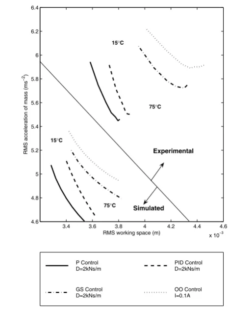
To compare control strategies, selected curves from each of the controller’s full conflict
diagram have been plotted on a single figure. The HILS experimental results are also
compared to equivalent simulations that incorporate the temperature dependant model
developed in Section 3. To begin, Figure 10 presents the conflict curves for selected
controller gains as a function of increasing temperature. The various controllers appear to be
equally sensitive to temperature variation but a significant difference is that the experimental
and simulated conflict curves appear in separate parts of the diagram. This phenomenon was
2005), and is not an indication of an invalid model. Using a validated model of the hydraulic
actuator, Batterbee et al. replicated this behaviour and illustrated good agreement between a
HILS experiment and a simulated HILS test (Batterbee et al., 2005). By subsequently
removing the actuator from the model, it was shown that the actuator dynamics (particularly
phase delay) had degraded performance but the relative performance between controllers
remained unchanged. This validated the use of the HILS method and is exactly the
observation that can be made in Figure 10. For example, despite the general shift in
performance levels, both simulated and experimental results display similar trends. Given the
result from this previous work, it was deemed unnecessary to include actuator dynamics in the
present study since its inclusion would have served to significantly complicate the numerical
analysis without adding significant value to the results.
To better compare the relative performance between controllers, Figure 11 plots the conflict
curves obtained at the highest and lowest temperatures as a function of the control parameter.
At low temperature (Figure 11(a)), except for the overall shift in the conflict curves (which
was explained previously), the simulated and experimental results display similar trends and
the relative performance between controllers is very similar. In general, P and PID control
have a similar performance, and outperform both GS and OO controllers. GS control
significantly outperforms OO control. At high temperature (Figure 11(b)), the conflict curve
trends between simulation and experiment compare favourably. The most noticeable
discrepancy is that GS control appears to have a better performance in the simulation, where it
can be seen to approach the P and PID controllers. This can be explained because the GS
controller gain terms were based on the numerical model. This model did not account for
frequency dependant behaviour (see Figure 6), which has resulted in sub-optimal controller
performance in the experiment. On the other hand, the use of feedback control desensitises
both simulation and experiment. In general, the trends of the experimental and simulated
conflict curves in Figure 11 show good agreement.
The above analysis has demonstrated a general shift to lower acceleration, and higher
suspension working space levels as the temperature rises. Furthermore, each controller
appears to be equally affected by this temperature variation. Given the good similarity
between the experimental and simulated results, the model can be regarded as a valid tool to
investigate the cause of this temperature sensitive performance.
Figure 12 presents a numerical sensitivity analysis that illustrates the individual effects of the
model parameters on the conflict diagram as the temperature rises. Here, each temperature
sensitive parameter (τy, Cpost and k) is varied in turn, whilst the remaining parameters are held
constant at their lowest temperature values. This analysis was carried out for each control
system, and for selected controller gains which were held constant. It can be observed that
the main affect of increasing the damper stiffness k is to decrease RMS acceleration. This is
because of the reduced hysteresis in the force/velocity response, which enhances the
controllability of the device. In contrast, the drop in yield stress τy degrades RMS
acceleration because of a reduction in device controllability. The post-yield viscosity Cpost
clearly has the most notable affect on all controllers, where rising temperature causes a
significant reduction in RMS acceleration and an increase in RMS working space. This
performance change occurs when the MR damper current is switched off (i.e. when an energy
input is required (Equation (2)), which explains why each controller is equally affected. The
lower viscosity reduces the off-state damping rate and hence the lower ‘clipped optimal’
control bound of the device. The energy dissipated when the skyhook law requires an energy
input is therefore minimised, and the controller behaves more closely to an ideal semi-active
acceleration, whilst increasing the RMS suspension working space as a result of the lower
off-state damping.
5
CONCLUSIONS
This paper has shown that the effects of temperature variation on an MR damper can be
significant. Temperature dependant behaviour was quantified between 15-75°C by
identifying the parameters in a physically meaningful MR damper model. Under certain
conditions, the analysis demonstrated a 34% drop in viscosity, a 22% reduction in yield stress,
and a 300% increase in damper stiffness with rising temperature. The model was validated
against experimental data for various temperatures and sinusoidal mechanical input
excitations. Good agreement was achieved although there was some frequency dependant
behaviour that was not accounted for by the model.
Control systems are often designed without this temperature sensitive behaviour in mind.
Consequently, the aim was to assess the influence of temperature on a broadband excited
single-degree-of-freedom (SDOF) mass isolator. Various controllers were compared in order
to assess their relative robustness against temperature uncertainty. These were proportional,
PID, gain scheduling and on/off control. Each system was configured to implement a
semi-active skyhook control law.
Control system experiments were performed at different temperatures using the
hardware-in-the-loop-simulation method. Here, the MR damper was physically tested, whilst the
remaining suspension system components were modelled in real-time. Each of the controllers
appeared to be equally sensitive to temperature. It was shown that the main affect of rising
temperature was to enhance the RMS acceleration, whilst degrading the RMS working space.
increase in RMS working space. The same conclusions were also drawn from a pure
simulation study, which utilised the temperature dependant MR damper model. The main
benefit of the model was that it enabled the cause of the observed behaviour to be explored in
greater detail.
A numerical sensitivity analysis demonstrated that the increase in damper stiffness enhanced
RMS acceleration, whilst the reduction in yield stress degraded it. The most significant affect
on RMS performance was a result of the change in fluid viscosity. This is because of the
change in the lower off-state damping level, which modifies the lower ‘clipped optimal’
control bound of the device. This lower bound determines how closely any control system
can perform to the ideal semi-active case, and thus all types of controller are equally affected.
Although it was not shown, it is also likely that sliding mode control, which is inherently
robust against parameter uncertainty, would be just as sensitive to temperature variations.
The choice of control strategy for smart fluid dampers still remains an unresolved problem,
and the present study also provided an opportunity to explore this further. Proportional and
PID control outperform the gain scheduling and on/off methods, although they are more
difficult to implement because of the requirement for force feedback. Furthermore,
proportional and PID control compare favourably. The added complexities when
implementing PID control (e.g. due to differentiated noise and integral wind up) may
therefore be difficult to justify. A gain scheduling control scheme is significantly superior to
on/off control, despite the relatively similar level of controller complexity. For example, both
controllers require similar sensing hardware and do not require force feedback.
Future work could focus on more complex control systems and ER/MR devices with different
modes of operation e.g. shear/mixed. Such investigations could yield different results
to investigate sliding mode control, which may be robust to temperature variation but would
still be subjected to changes in the off state damping.
ACKNOWLEDGEMENTS
The authors would like to acknowledge the support of the EPSRC under grant references
EP/D078601/1 (DC Batterbee and ND Sims) and GR/S49841/01 (ND Sims).
REFERENCES
Batterbee, D.C. and Sims, N.D. 2005. "Vibration isolation using smart fluid dampers: A benchmarking study." Smart Structures and Systems, 1(3):235-256.
Batterbee, D.C. and Sims, N.D. 2007. "Hardware-in-the-loop-simulation of
magnetorheological dampers for vehicle suspension systems", Proceedings of the Institution of Mechanical Engineers, Part I: Journal of Systems and Control Engineering, 221(2):265-278.
Batterbee, D.C.Sims, N.D. and Plummer, A. 2005. "Hardware-in-the-loop-simulation of a vibration isolator incorporating magnetorheological fluid damping", 2nd ECCOMAS Thematic Conference on Smart Structures and Materials, Lisbon, Portugal.
Choi, S.-B.Song, H.J.Lee, H.H.Lim, S.C.Kim, J.H. and Choi, H.J. 2003. "Vibration control of a passenger vehicle featuring magnetorheological engine mounts", International Journal of Vehicle Design, 33(1-3):2-16.
Choi, S.B.Han, S.S. and Han, Y.M. 2005. "Vibration control of a smart material based damper system considering temperature variation and time delay", Acta Mechanica, 180 (1-4):73-82.
Delphi Press Release 2006a. "Delphi's MagneRide semi-active suspension helps increase comfort and handling on the new Audi TT",
http://delphi.com/news/pressReleases/pressReleases_2006/pr_2006_06_01_001/. Delphi Press Release 2006b. "Ferrari 599 GTB driving experience boosted by Delphi
Technology", http://delphi.com/news/pressReleases/pressReleases_2006/pr72389-03012006/.
Dogruoz, M.B.Wang, E.L.Gordaninejad, F. and Stipanovic, A.J. 2003. "Augmenting heat transfer from fail-safe magneto-rheological fluid dampers using fins", Journal of Intelligent Material Systems and Structures, 14(2):79-86.
Du, H.Yim Sze, K. and Lam, J. 2005. "Semi-active H∞ control of vehicle suspension with magneto-rheological dampers", Journal of Sound and Vibration, 283(3-5):981-996. Gordaninejad, F. and Breese, D.G. 1999. "Heating of magnetorheological fluid dampers",
Journal of Intelligent Material Systems and Structures, 10(8):634-645.
Instron Structural Testing Systems 2007. 825 University Ave., Norwood, MA 02062-2643, USA, http://www.instron.com.
Karnopp, D.Crosby, M.J. and Harwood, R.A. 1974. "Vibration control using semi-active force generators." Journal of Engineering for Industry, 96(2):619-626.
Kepco Inc. 2007. 131-138 Sanford Avenue, Flushing, NY 11352, USA,
Lee, H.-S. and Choi, S.-B. 2000. "Control and response characteristics of a magneto-rheological fluid damper for passenger vehicles", Journal of Intelligent Material Systems and Structures, 11(1):80-87.
Liu, Y.Gordaninejad, F.Evrensel, C.A.Dogruer, U.Yeo, M.-S.Karakas, E.S. and Fuchs, A. 2003. "Temperature dependent skyhook control of HMMWV suspension using a failsafe magneto-rheological damper", SPIE Annual International Symposium on Smart Structures and Materials, 5054:332-340.
Lord Corporation 2007. Materials Division, 406 Gregson Drive, Cary, NC 27511, USA,
http://www.lord.com.
Simon, D. and Ahmadian, M. 2001. "Vehicle evaluation of the performance of
magnetorheological dampers for heavy truck suspensions", Journal of Vibration and Acoustics, 123(3):365-375.
Sims, N.D. 2006. "Limit cycle behaviour of smart fluid dampers under closed-loop control", Journal of Vibration and Acoustics, 128(4):413-428.
Sims, N.D.Holmes, N.J. and Stanway, R. 2004. "A unified modelling and model updating procedure for electrorheological and magnetorheological dampers", Smart Materials and Structures, 13:100-121.
Sims, N.D.Peel, D.J.Stanway, R.Bullough, W.A. and Johnson, A.R. 1999. "Controllable viscous damping: An experimental study of an electrorheological long stroke damper under proportional feedback control", Smart Materials and Structures, 8(5):601-605. Sims, N.D.Stanway, R.Peel, D.J.Bullough, W.A. and Johnson, A.R. 2000. "Smart fluid
damping: Shaping the force/velocity response through feedback control." Journal of Intelligent Material Systems and Structures, 11(12):945-949.
Spencer Jr., B.F.Dyke, S.J.Sain, M.K. and Carlson, J.D. 1997. "Phenomenological model for magnetorheological dampers", Journal of Engineering Mechanics, 123(3):230-238. Xia, P.-Q. 2003. "An inverse model of MR damper using optimal neural network and system
identification", Journal of Sound and Vibration, 266(5):1009-1023.
Yoshida, O. and Dyke, S.J. 2004. "Seismic control of a nonlinear benchmark building using smart dampers", Journal of Engineering Mechanics, 130(4):386-392.
Ziegler, J.G. and Nichols, N.B. 1942. "Optimum settings for automatic controllers", Transactions of the ASME, 64:759-768.
Current Viscosity change per degree Viscosity Intercept Yield force change per degree Yield Force Intercept Stiffness change per degree Stiffness intercept
(A) (Ns/m/°C) (Ns/m) (N/°C) (N) (kN/m/°C) (kN)
0 -6.78 1400 0.19 41 150 1500
0.2 -7.07 1265 -0.53 331 " "
0.4 -8.11 1451 -1.87 766 " "
0.6 -8.74 1616 -3.47 1178 " "
0.8 -8.91 1734 -5.26 1481 " "
[image:22.595.102.522.576.709.2]1 -9.43 1824 -6.42 1667 " "
Instron Controller Host PC
Target PC
Kepco BOP Current Amplifier N.I Interface
Board
Lord MR Damper and Cooling Coil
[image:23.595.76.538.99.407.2]Instron servo-hydraulic actuator Load Cell
Figure 1: Photograph of the MR damper test facility.
Accumulator
Annular orifice Piston seal
Coil
Rod seal
Magnetic flux lines
[image:23.595.86.510.532.648.2]−0.4 −0.2 0 0.2 0.4 0.6 −3000 −2000 −1000 0 1000 2000 3000 Velocity (m/s) Force (N) (a)
T = 14 °C T = 71 °C
T = 37 °C
−10 −5 0 5 10
[image:24.595.95.494.95.344.2]−3000 −2000 −1000 0 1000 2000 3000 Displacement (mm) Force (N) (b)
Figure 3: MR damper force/velocity (a) and force/displacement (b) curves at different temperatures. 10mm, 8Hz sinusoidal excitation, I = 1A.
Cpre
Cpost
Fy
) , (x1 I Fd = χ &
Quasi-steady damper velocity x&1
Spring
displacement = x2 – x1
)
(x2 x1
k
Fs = −
k
m1
x1 x2
k
F
) , (x&1 I
χ
[image:24.595.122.465.424.633.2]I=0A I=0.2A I=0.4A
I=0.6A I=0.8A I=1A
I=2A
10 20 30 40 50 60 70 80 600
800 1000 1200 1400 1600 1800
Post Yield Viscosity (Ns/m)
Temperature (°C) (a)
0 20 40 60 80 0
250 500 750 1000 1250 1500
Temperature (°C)
Yield Force (N)
(b)
20 40 60 80 0
2 4 6 8 10 12 14
Stiffness (MN/m)
[image:25.595.91.493.94.344.2]Temperature (°C) (c)
Figure 5: Identified model parameters as a function of temperature and current. (a) Post-yield viscosity
Cpost and (b) yield force Fy, and (c) damper stiffness k. Figures 5(a) and 5(b) show data up to 1A. Figure
(a) (b)
−0.5 0 0.5
−2000 −1000 0 1000 2000
Velocity (m/s)
Force (N)
−0.5 0 0.5
−2000 −1000 0 1000 2000
Velocity (m/s)
Force (N)
(c) (d)
−0.1 0 0.1
−2000 −1000 0 1000 2000
Velocity (m/s)
Force (N)
−0.1 0 0.1
−2000 −1000 0 1000 2000
Velocity (m/s)
[image:26.595.76.514.78.603.2]Force (N)
Figure 6: Experimental (solid lines) and simulated (dotted lines) force/velocity curves for 0, 0.4, and 0.8A.
(a) 10mm-8Hz, Tavg = 15°C, (b) 10mm-8Hz, Tavg = 75°C, (c) 5mm-4Hz, Tavg = 15°C and (d) 5mm-4Hz,
Manifold Servo-valves Hydraulic power supply Lord MR damper IST 8400 Controller IST Actuator Position feedback MR actuation current Kepco Amplifier
Analogue inputs and outputs
INTERFACE BOARD TARGET PC
RUNNING REAL-TIME SIMULATION
N.I. DAQ Card
D/A Converter A/D Converter Download C-code Upload HILS data Transducers
(Load cell, LVDT)
Desired actuator position
HOST PC RUNNING XPC TARGET
•Model of ‘simulated’ isolator components and controller
[image:27.595.122.471.114.428.2]Measurement data Desired MR damper current Damper force (from hardware) M Kiso C-COMPILER
Figure 7: Schematic diagram of the HILS testing facility (see Figure 1 for photograph).
(a) (b)
‘Skyhook’ damper M Base Excitation xb Response xm Spring Stiffness,
K = 78.5kN/m
MR damper,
ζmin ≈ 0.2
Mass, M = 80kg
K
[image:27.595.105.492.528.668.2]3.2 3.4 3.6 3.8 4 4.2 4.4 4.6 x 10⁻³ 5.4 5.5 5.6 5.7 5.8 5.9 6 6.1 6.2 6.3 6.4
RMS working space (m)
RMS acceleration of mass (ms
−
2)
15.5°C
22.9°C
33.2°C 43.1°C
[image:28.595.127.464.96.370.2]53.6°C 63.8°C 74.4°C 1kNs/m 1.5kNs/m 2kNs/m 2.5kNs/m 3kNs/m 3.5kNs/m
Figure 9: Experimental conflict curves for proportional skyhook control.
`
P Control
D=2kNs/m PID ControlD=2kNs/m
GS Control
D=2kNs/m OO ControlI=0.1A
3.4 3.6 3.8 4 4.2 4.4 4.6
x 10−3
4.6 4.8 5 5.2 5.4 5.6 5.8 6 6.2 6.4
RMS working space (m)
RMS acceleration of mass (ms
−
2)
Experimental
Simulated
15°C
75°C
15°C
75°C
[image:28.595.173.406.404.721.2]3 3.2 3.4 3.6 3.8 4 4.2 4.4 4.6 4.8 5 x 10⁻³ 4.5 5 5.5 6 6.5 7
RMS working space (m)
RMS acceleration of mass (ms
−
2 )
(b)
P Control PID Control
GS Control OO Control
3 3.2 3.4 3.6 3.8 4 4.2 4.4 4.6 4.8 5 x 10⁻³ 4.5 5 5.5 6 6.5 7
RMS working space (m)
RMS acceleration of mass (ms
[image:29.595.80.516.87.366.2]− 2) (a) Simulated Experimental Direction of increasing gain Simulated Experimental Direction of increasing gain
Figure 11: Conflict curves as a function of the control parameter for (a) low and (b) high temperature. D = 1-4kNsm-1, Imax=0-0.2A.
Variable yield stress
Variable damper stiffness
Variable post−yield viscosity
3.2 3.3 3.4 3.5 3.6 3.7 3.8
x 10−3 4.5 4.6 4.7 4.8 4.9 5 5.1 5.2 5.3 5.4 5.5
RMS working space (m)
RMS acceleration of mass (ms
− 2) PID D=2kNs/m GS D=3.5kNs/m OO Imax=0.1A
P D =2kNs/m
[image:29.595.197.404.420.731.2]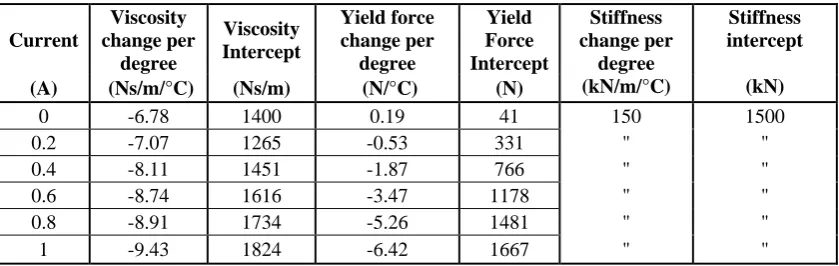


![Genetic correlations among psychiatric and immune-related phenotypes based on genome-wide association data [preprint]](data:image/gif;base64,R0lGODlhAQABAIAAAP///wAAACH5BAEAAAAALAAAAAABAAEAAAICRAEAOw==)