Image based automatic vehicle damage detection

(1)

Srimal Jayawardena

A thesis submitted for the degree of

Doctor of Philosophy at

The Australian National University

(2)

(3)

person nor material which to a substantial extent has been accepted for the award of any other

degree or diploma of a university or other institute of higher learning, except the following: (1)

I received much advice from my supervisory panel, Marcus Hutter, Stephen Gould, Hongdong

Li and Richard Hartley for the preparation of the thesis as a whole, and technical advice from

Nathan Brewer to implement some of the work presented in Chapter 4; (2) Section 3.3 was

based on work done collaboratively with Di Yang.

. . . .

Srimal Jayawardena

(4)

(5)

Research Outcomes

The following research outcomes have resulted from the work presented in this thesis.

Publications

• JAYAWARDENA, S.; HUTTER, M.; AND B REWER , N., 2011. A novel illumination-invariant loss for monocular 3D pose estimation. In Digital Image Computing

Tech-niques and Applications (DICTA), 2011 International Conference on, 37–44.

• JAYAWARDENA, S.; Y ANG , D.; AND H UTTER, M., 2011. 3D model assisted image

segmentation. In Digital Image Computing Techniques and Applications (DICTA), 2011

International Conference on, 51–58.

• JAYAWARDENA, S.; GOULD , S.; LI, H.; AND HUTTER , M., 2013. 3D epipolar

ge-ometry recovery from images dominated by highly reflective and largely homogeneous

regions. In Computer Vision and Pattern Recognition (CVPR), 2014 IEEE Conference

on. (Under Review)

• JAYAWARDENA, S.; BREWER, N.; HUTTER, M.; GOULD , S.; LI , H.; AND

HART-LEY , R. 3D CAD model based monocular pose recovery. Machine Vision and

Appli-cations. (Under Review).

Software

Prototype software developed based on this research have been handed over to the industry

partnerControlexpert, which is protected by a non-disclosure agreement.

Invited talks

(6)

2011

• CVC Lab, Barcelona, Spain – November 2011

(7)

(8)

(9)

unintentional.

I would like to graciously acknowledge our industry partner Controlexpert, for funding my work and scholarship. I would also like to thank the Australian National University for

providing my tuition fee scholarship.

I am very grateful to my primary supervisor and panel chair, Prof. Marcus Hutter. Thank

you for helping me to see problems in completely new ways and turn impossibilities into

possibilities. I cannot thank you enough for honing my research skills, as well as for your

friendship, guidance and support throughout my PhD candidature.

I had the incredible good fortune to be advised by Prof. Richard Hartley. Thank you for

your clear direction and candid opinion which saved me a lot of valuable time; time which

might have otherwise been used unproductively. Thank you very much for your critical

feed-back which helped shape my research.

I am deeply indebted to Dr. Stephen Gould for his valuable mentoring and guidance.

Thank you for being more than approachable; for always being there. You have helped me

learn much; both from our individual meetings and through the reading group sessions which

not only broadened my research horizons but also my network of colleagues.

I am truly grateful to Dr. Hongdong Li for providing valuable guidance during my

candi-dature. Much have I benefited from your advice, guidance and critical feedback which helped

me focus on important aspects of scientific research. Thank you very much.

Many other academic and technical staff at the ANU have been very helpful during my

PhD candidature. Thank you, Prof. Robert Mahony for allowing me to use the 3D printer and

also thank you Alex Martin for helping me with the 3D printing. Thank you very much Hugh

Fisher for introducing me to OpenGL during my first year and for liberally sharing your copies

of the OpenGL super bibles. Many thanks to everyone who’s critical feedback during my talks

have shaped my research in one way or another.

I have greatly benefited from discussions with my friends and fellow students. Thank you

Di, Nathan, Jan, Phuong, Wen and many others whom I have not mentioned specifically. Many

(10)

procedures, processed funds in time and who saw to it that PhD students were lavished with

free food whenever possible.

My research would not have been possible if not for many friends who graciously allowed

me to photograph their damaged vehicles. Thank you Heather, Revantha, Ali and many others

whom I am incapable of enumerating at this moment.

Settling down in Canberra would not have been the same if not for the many friends in

Canberra who welcomed us warmly and helped us settle in. Thank you very much Sean and

Dulamani for your kind friendship, the gentle introduction to Canberra and also for the

de-licious meals which saved me much cooking woes. A special thank you to our two foster

families in Canberra. Thank you very much Indra and Ranjit Gajanayake, for your loving care;

particularly for hosting Dinelie’s birthday party three years in a row, starting from her first

birthday. Thank you very much Kumu and Vasanthe Vithanage for your help; thank you Kumu

Aunty for babysitting Dinelie and practically being a grandmother to her. Many thanks to our

friends at the Church of Christ, Lyons for their supportive fellowship.

I would like to thank my wonderful parents; thank you for all your love, support and

constant encouragement over the past three decades. I am also thankful to my wife’s parents

and sister for their support and hospitality. I owe much gratitude to my loving wife Nirasha;

without your constant support and encouragement I may have never completed my PhD. While

I simply had to do a PhD, you had to run a home with a toddler and a PhD student; a very

demanding and challenging task which you did exceptionally well. Thank you for leaving

our comfortable lives back in Colombo to embark on this wonderful adventure; an adventure

which we will cherish for years to come. To our sweet little daughter Dinelie for providing me

a healthy distraction. As much as your tantrums and late night wakeup calls challenged my

(11)

age assessment and insurance claim processing done automatically. However, such a solution

remains a challenging task due to a number of factors. For a start, the scene of the accident is

typically an unknown and uncontrolled outdoor environment with a plethora of factors beyond

our control including scene illumination and the presence of surrounding objects which are not

known a priori. In addition, since vehicles have very reflective metallic bodies the photographs

taken in such an uncontrolled environment can be expected to have a considerable amount

of inter object reflection. Therefore, the application of standard computer vision techniques

in this context is a very challenging task. Moreover, solving this task opens up a fascinating

repertoire of computer vision problems which need to be addressed in the context of a very

challenging scenario. This thesis describes research undertaken to address the problem of

au-tomatic vehicle damage detection using photographs. A pipeline addressing a vertical slice of

the broad problem is considered while focusing on mild vehicle damage detection.

We propose to use 3D CAD models of undamaged vehicles which are used to obtain ground

truth information in order to infer what the vehicle with mild damage in the photograph should

have looked like, if it had not been damaged. To this end, we develop 3D pose estimation

algorithms to register an undamaged 3D CAD model over a photograph of the known

dam-aged vehicle. We present a 3D pose estimation method using image gradient information of

the photograph and the 3D model projection. We show how the 3D model projection at the

recovered 3D pose can be used to identify components of a vehicle in the photograph which

may have mild damage. In addition, we present a more robust 3D pose estimation method by

minimizing a novel illumination invariant distance measure, which is based on a Mahalanobis

distance between attributes of the 3D model projection and the pixels in the photograph.

In principle, image edges which are not present in the 3D CAD model projection can be

considered to be vehicle damage. However, since the vehicle body is very reflective, there is a

large amount of inter object reflection in the photograph which may be misclassified as damage.

In order to detect image edges caused by inter object reflection, we propose to apply multi-view

geometry techniques on two photographs of the vehicle taken from different view points. To

(12)

photographs which are dominated by large reflective and mostly homogeneous regions.

The performance of the proposed methods are experimentally evaluated on real photographs

using 3D CAD models of varying accuracy. We expect that the research presented in this thesis

will provide the groundwork for designing an automatic photograph based vehicle damage

de-tection system. Moreover, we hope that our method will provide the foundation for interesting

(13)

1 Introduction 1

1.1 Objective . . . 1

1.2 Motivation . . . 1

1.3 Challenges . . . 2

1.4 Contribution . . . 3

1.4.1 Monocular 2D/3D pose estimation . . . 3

1.4.2 3D model assisted segmentation . . . 3

1.4.3 Reflection detection . . . 4

1.4.4 Obtain reliable point correspondences across photographs with largely reflective and homogeneous regions . . . 4

1.5 Thesis outline . . . 4

2 Background and Related Work 7 2.1 Pose estimation . . . 7

2.1.1 Image gradient based methods . . . 9

2.1.2 Feature based methods . . . 9

2.1.3 Distance measures . . . 10

2.1.4 Optimization for pose estimation . . . 10

2.1.4.1 Downhill Simplex . . . 11

2.2 Two-view geometry . . . 13

2.3 Point correspondences between images . . . 16

2.4 Chapter summary . . . 17

3 Pose Estimation and Segmentation 19 3.1 Introduction . . . 19

3.2 3D model registration . . . 20

3.2.1 Gradient based distance measure . . . 20

(14)

3.2.3 Gaussian smoothing . . . 22

3.2.4 Choosing the normp . . . 22

3.2.5 Representation of the pose . . . 22

3.2.5.1 Perspective projection . . . 26

3.2.6 Distance measure optimization . . . 27

3.2.6.1 The optimizer . . . 27

3.2.6.2 Normalised pose parameters . . . 27

3.2.6.3 Initialization . . . 29

3.2.6.4 Background removal . . . 29

3.3 Contour detection . . . 30

3.4 Results . . . 31

3.4.1 Sensitivity of the estimated pose to the initial pose . . . 32

3.4.2 Pose and segmentation of real photographs . . . 35

3.4.2.1 Pose estimation . . . 35

3.4.2.2 Segmentation . . . 35

3.4.2.3 Accuracy . . . 38

3.4.2.4 Benchmark tests . . . 38

4 Robust Pose Estimation 41 4.1 Introduction . . . 41

4.1.1 Motivation . . . 41

4.1.2 Main contribution . . . 43

4.2 Registering a 3D Model over a 2D photograph . . . 44

4.2.1 Problem statement . . . 44

4.2.2 Theoretical formulation . . . 45

4.2.3 Lambertian reflection model . . . 45

4.2.4 Illumination invariant distance measure . . . 46

4.3 Derivation of the illumination invariant distance measure . . . 47

4.3.1 Notation . . . 47

4.3.2 Unknown noisy relationship . . . 47

4.3.3 Linear relationship . . . 48

4.3.4 Linear invariant distance . . . 49

4.3.5 Explicit expression of the distance measure . . . 49

(15)

4.6.1 Sensitivity to the initial pose . . . 53

4.6.2 Results on real photographs . . . 55

4.7 Implementation details . . . 57

4.7.1 3D rendering . . . 58

4.7.2 Running times . . . 58

5 Reliable Point Correspondences 61 5.1 Introduction . . . 61

5.2 Problem formulation and proposed solution . . . 63

5.2.1 Putative point matches . . . 63

5.2.2 Selecting candidate points . . . 63

5.2.3 Edges in the image . . . 65

5.2.4 Sift on edge points . . . 65

5.2.5 Edge feature ambiguities . . . 65

5.2.6 Recovery of the epipolar geometry (EPG) . . . 66

5.2.7 RANSAC . . . 66

5.2.8 Spatial Constraint . . . 67

5.3 Experiments . . . 67

5.3.1 Quantitative results and comparison with baseline methods . . . 67

5.3.2 Compared methods . . . 69

5.3.3 Qualitative results . . . 69

5.3.4 Matching Distance . . . 75

5.3.5 Scale . . . 75

6 Reflection Edge Detection 81 6.1 Introduction . . . 81

(16)

6.2.1 Problem formulation . . . 83

6.2.1.1 Image warping via texture mapping . . . 84

6.2.1.2 A simple distance measure . . . 85

6.2.1.3 Offset based distance measure . . . 87

6.2.1.4 A distance measure accounting for local shape information . 89 6.2.1.5 Adjoining pixel color as a feature . . . 90

6.2.2 Experiments . . . 90

6.2.2.1 Statistics used for evaluating the performance . . . 91

6.2.2.2 Evaluating the overall performance . . . 92

6.2.2.3 Qualitative results . . . 93

6.2.3 Limitations . . . 93

6.2.3.1 Point distances . . . 93

6.2.3.2 Fragmented edges . . . 95

6.2.3.3 Image warping . . . 97

6.3 Reflection classification via homography estimation . . . 97

6.3.2 Problem formulation . . . 98

6.3.3 Proposed solution . . . 99

6.3.4 Symmetric Transfer Error (STE) . . . 99

6.3.5 Estimating the homography transformationHand the STE . . . 99

6.3.6 Experiments and quantitative evaluation of results . . . 101

6.3.6.1 Learned threshold and cross-validation . . . 101

6.3.6.2 Logistic classifier . . . 101

6.3.6.3 Overall performance . . . 103

6.3.7 Qualitative evaluation of results . . . 103

6.3.8 Photographs of complete vehicles . . . 105

7 Conclusions and Future Directions 109 7.1 Summary and contributions . . . 109

7.1.1 Monocular 2D/3D pose estimation . . . 109

7.1.2 3D model assisted segmentation . . . 110

7.1.3 Reflection detection . . . 110

(17)

7.2.4 Other components of the project . . . 112

7.3 Conclusions . . . 112

A Distance Measure Landscapes for a Synthetic and a Real Photograph 113

B Epipolar Geometry Recovery Results 137

(18)

(19)

2.1 The simplex for a 2D function . . . 11

2.2 Corresponding points and epipolar geometry . . . 14

3.1 Result and benchmark comparison . . . 20

3.2 Visualisations of surface normal components for the Mazda 3 withn=0 . . . 23

3.3 Visualisation of image gradients of car photographs . . . 24

3.4 Overlays ofGN(θ)andGN(θ)for Mazda 3 photographs . . . 25

3.5 1-norm and2-norm gradient based distance measure landscapes . . . 25

3.6 Pose representation . . . 26

3.7 Rendering with perspective projection . . . 28

3.8 Sensitivity analysis plots - 1 . . . 32

3.9 Correct initial pose, background removal and the resulting incorrect final pose . 34 3.10 Pose estimation results . . . 36

3.11 Pose estimation results - close ups . . . 37

3.14 Results for a semi-profile view . . . 40

4.1 Results using a laser scanned 3D Model . . . 42

4.2 Distance measure landscapes for synthetic and real photographs . . . 52

4.5 3D CAD Models . . . 56

4.6 Results using cheap 3D CAD models from the Internet . . . 57

5.1 Limitations in existing point correspondence approaches . . . 62

5.2 Quantitative evaluation on the DAISY dataset . . . 68

5.3 Results of our method on a pair of images from the Middlebury dataset . . . 70

(20)

5.5 Results from our method . . . 72

5.6 Results of Daisy on Harris key-points . . . 73

5.7 Results of Daisy on SIFT key-points . . . 73

5.8 Results of SIFT key point detection and matching . . . 74

5.9 Our EPG results for a car door . . . 76

5.10 Recovered EPG and inlier point correspondences from a photograph of a highly reflective building . . . 77

5.11 Our EPG results for an SUV . . . 78

5.12 Our EPG results for the rear of a car . . . 79

6.1 Types of image edges . . . 83

6.2 Motivation based on relative motion . . . 84

6.3 Image warping using a 3D CAD model and texture mapping . . . 86

6.4 Different possible ordering of edge points . . . 87

6.5 Distance measure with an offset . . . 88

6.6 Predicted edge points . . . 94

6.7 Limitations of the distance measure . . . 95

6.8 Area based distance measure . . . 96

6.9 Fragmented edges . . . 96

6.10 Motivation based on apparent depth . . . 98

6.11 Mode ofdSTEvalues . . . 102

6.12 PR curve . . . 104

6.13 Predicted edge points . . . 106

A.1 Photographs used to generate distance measure landscapes . . . 114

A.2 Distance measure landscape with respect toµx andµy . . . 115

A.3 Distance measure landscape with respect toµx andδx . . . 116

A.4 Distance measure landscape with respect toµx andδy . . . 117

A.5 Distance measure landscape with respect toµx andφx . . . 118

A.6 Distance measure landscape with respect toµx andφy. . . 119

A.7 Distance measure landscape with respect toµx and f . . . 120

A.8 Distance measure landscape with respect toµyandδx . . . 121

A.9 Distance measure landscape with respect toµyandδy . . . 122

A.10 Distance measure landscape with respect toµyandφx. . . 123

(21)

A.16 Distance measure landscape with respect toδxand f . . . 129

A.17 Distance measure landscape with respect toδyandφx . . . 130

A.18 Distance measure landscape with respect toδyandφy . . . 131

A.19 Distance measure landscape with respect toδyand f . . . 132

A.20 Distance measure landscape with respect toφxandφy. . . 133

A.21 Distance measure landscape with respect toφxand f . . . 134

A.22 Distance measure landscape with respect toφyand f . . . 135

B.1 Results on the car dataset. Subfigures are explained in Table B.1. Color code: cyan lines - epipolar lines, yellow dots - matched points, magenta lines - point correspondences. Best viewed in color. . . 139

(22)

cyan lines - epipolar lines, yellow dots - matched points, magenta lines - point

correspondences. Best viewed in color. . . 147

B.10 Results on the car dataset. Subfigures are explained in Table B.1. Color code:

(23)

(24)

(25)

6.1 Performance statistics (image warping) . . . 92

6.2 Performance statistics (homography) . . . 103

B.1 Descriptions of subfigures. . . 137

(26)

(27)

1 .

1 Objective

Automatically detecting vehicle damage after an accident using photographs taken at the

acci-dent scene, is potentially a very useful yet challenging task. Moreover, solving this task opens

up a fascinating repertoire of computer vision problems which need to be addressed in the

con-text of a very challenging scenario. For instance, since vehicles have very reflective metallic

bodies and the photographs are taken in an uncontrolled environment, it is very challenging to

apply standard computer vision techniques in this context.

This research was done forControlexpert, an industry partner company based in Germany. The industry partner is in the business of processing insurance claims and therefore, sees a lot

of potential in automating the process of handling insurance claims for vehicles which suffer

mild damage following an accident.

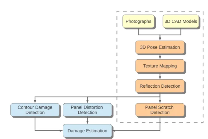
The overall objective of this research is to be able to automatically detect mild damage in

vehicles using photographs taken at the scene of the accident. The photographs would typically

be taken from a device such as a mobile phone. Anticipated components of this ambitious task

and their interdependencies are illustrated in Figure 1.1. The work presented in this thesis

addresses a vertical slice of the project where the scope is limited to detecting scratch damage

in the vehicle as indicated by the dashed box in Figure 1.1.

1 .

2 Motivation

A vehicle meets with an accident. At the moment what happens next would be as follows.

The vehicle owners/drivers call the relevant insurance companies. They wait till the insurance

agents arrive at the scene of the accident. The agents take photographs of the accident scene

and forms need to be filled out. A lot of time is wasted while all this takes place. More

importantly the insurance companies spend a lot of money in employing staff to drive down to

(28)

3D CAD Models

Photographs

3D Pose Estimation

Texture Mapping

Reflection Detection

Panel Scratch Detection

Panel Distortion Detection

Contour Damage Detection

Damage Estimation

[image:28.595.99.438.108.334.2]

Damage Estimation

Figure 1.1: Components of the overall project with the components within the vertical slice addressed by this research indicated by the dashed box

the scene of the accident. The grand vision of this work therefore, is as follows. In contrast to

the previous scenario, with the proposed technology, the driver would simply take photographs

of the damaged vehicle which will be directly uploaded to the company server via a mobile

phone application and drive away. The photographs will be automatically assessed for damage

using advance computer vision and machine learning techniques, thereby greatly automating

the insurance claims process; saving a lot of time and money. Other benefits which could

also result from such an automatic system include reducing human error, avoiding subjective

decisions by human damage assessors and preventing fraud.

1 .

3 Challenges

The fact that the photographs are taken in an uncontrolled environment makes this task very

challenging. The scene illumination is very complex and hard to predict before hand. To make

things worse, vehicles typically have very reflective metallic bodies which cause a lot of inter

object reflections. These can be easily confused as damage, even by trained human experts. In

addition, since the photographs are taken from a customer’s mobile phone at the scene of the

accident, information about the camera setup is not known a priori. If information about the

(29)

1 .

4 Contribution

The motivation behind the proposed solution is to use a library of 3D CAD models of

undam-aged vehicles as ground truth information, in order to detect mild damage in a vehicle using

photographs. The ground truth 3D model needs to be registered over the photograph in order

to know what the vehicle in the photograph should have looked like if it had not been

dam-aged. In principle, image edges which are not present in the 3D CAD model projection can

be considered to be vehicle damage. However, since the vehicle body is very reflective, there

is a large amount of inter object reflection in the photograph which may be misclassified as

damage. Therefore, we use robust image feature detection and matching combined with

multi-view geometry techniques to detect inter object reflections in vehicles using photographs taken

from two views. Based on this rationale, we make the following contributions.

1.4.1 Monocular2D/3D pose estimation

We propose methods to recover the 3D pose of a known object in a given image (in particular

the pose of a known vehicle). In other words, we propose methods to obtain the 3D pose

parameters required to register a 3D CAD model of a known object over a photograph of the

object. To this end we derive distance measures which can be optimized with respect to the

3D pose parameters, in order to obtain the final 3D pose. We present two methods; one in

Chapter 3 and a more robust method in Chapter 4. The work was published in Jayawardena

et al. [37] and Jayawardena et al. [36], respectively. An extended version of the pose estimation

work, Jayawardena et al. [34] is currently under review.

1.4.2 3D model assisted segmentation

We propose a method to use the 3D CAD model projection to help in segmenting and

sepa-rating components of a vehicle body like the doors and fenders which are separated by weak

boundary cues (e.g., parts consisting of the same color and paint). This work which is presented

(30)

We propose methods to detect reflections appearing on the vehicle body using photographs of

the vehicle taken from two views. Using this approach, we separate image edges caused by

reflections from edges on the surface of vehicle panels. Since image edges on the surface of

the vehicle can be identified with the aid of the 3D CAD model projection as developed in

Chapter 3, identifying reflection edges helps isolate mild damage to the vehicle in the form of

scratches, peeled off paint, etc,. The reflection detection work which is explained in detail in

Chapter 6.2, relies on the work presented in Chapter 5 which is used to obtain reliable point

correspondences between the two photographs.

1.4.4 Obtain reliable point correspondences across photographs with largely

reflective and homogeneous regions

Photographs of vehicles are dominated by large amounts of inter object reflections as the

metal-lic vehicle body tends to be very reflective. Apart from this, the body of a vehicle tends to have

large homogeneous regions which are relatively feature impoverished. Given photographs

from two views of the vehicle, traditional methods find it challenging to obtain

correspond-ing points across the images that are reliable enough to perform typical structure from motion

tasks like fitting a homography or estimating the epipolar geometry of the scene. We propose

a method which can find point correspondences that are reliable enough for our work using an

approach which compares feature descriptors along image edges in Chapter 5. A publication

based on this work, Jayawardena et al. [35], is currently under review.

1 .

5 Thesis outline

The remainder of this thesis is organized as follows.

In Chapter 2 we present the technical background and a review of related work. This

includes related work done on pose estimation, work related to the recovery of epipolar

ge-ometry and related work on obtaining reliable point matches between photographs of a scene

taken from two views.

We discuss a 3D pose estimation method and our model assisted segmentation method

in Chapter 3. Experiments are conducted to evaluate the sensitivity of the estimated pose to

variations in the initial pose used to seed the optimizer. Results on real car images are compared

with baseline methods.

In Chapter 4 we present our novel illumination invariant distance measure which can be

(31)

fol-The reflection detection approach is discussed in Chapter 6.2. Following the theoretical

formulation, we include reflection detection results on a dataset of real vehicle photographs.

The proposed approach utilizes a method to obtain reliable point correspondences across

pho-tographs with largely reflective and homogeneous regions which is presented in Chapter 5.

(32)

(33)

In this chapter we introduce background material necessary to discuss the work in the chapters

that follow. In doing so we also review related work. As we intend to register a 3D CAD

model of a vehicle over a photograph in our work, we begin this chapter by reviewing

litera-ture on 3D pose estimation. Since we use photographs obtained from two different views to

detect reflections on the vehicle surfaces, we proceed to discuss two view geometry and point

correspondences across two views, in the remainder of this chapter.

2 .

1 Pose estimation

Interest in the use of 3D CAD models has a long history in computer vision. For the sake of

completeness, we include literature spanning at least 50 years from now, when such research

spurred a lot of interest. Although widely used in computer graphics, the use of realistic 3D

CAD models (i.e., 3D models consisting of a large number of polygons) in computer vision

research has been limited by computational constraints. Hence, computer vision researchers

tend to have resorted to other computationally feasible methods over the more recent past. With

the advent of more powerful computing resources, realistic 3D CAD models are becoming

popular [9, 8] once more.

We begin our discussion based on a survey by Chin and Dyer [15] which shows that model

based object recognition algorithms generally fall into three categories based on the type of

object representation used; namely, 2D representations, 2.5D representations and 3D

represen-tations.

2Drepresentations store the information of a particular 2D view of an object (a characteristic

view) as a model and use this information to identify the object from a 2D image. Global

feature methods have been used by Gleason and Algin [25] to identify objects like spanners

and nuts on a conveyor belt. Such methods use features such as the area, perimeter, number of

holes visible and other global features to model the object. Structural features like boundary

(34)

graph method has been used by Yachida and Tsuji [90] to match objects to a 2D model using

graph matching techniques. These 2D representation based algorithms require prior training

of the system using a ‘show by example’ method.

2.5Dapproaches are also viewer centered, where the object is known to occur in a particular

view. They differ from the 2D approach as the model stores additional information such as

intrinsic image parameters and surface-orientation maps. The work done by Poje and Delp [70]

explain the use of intrinsic scene parameters in the form of range (depth) maps and needle (local

surface orientation) maps. Shape from shading [31] and photometric stereo [87] are some other

examples of the 2.5D approach used for the recognition of industrial parts.

A range of techniques for such 2D/2.5D representations are described by Forsythe and

Ponce [22], by posing the object recognition problem as a correspondence problem. These

methods obtain a hypothesis based on the correspondences of a few matching points in the

image and the model. The hypothesis is validated against the remaining known points.

3Dapproaches are utilized in situations where the object of interest can appear in a scene from

multiple viewing angles. Common 3D representation approaches can be either an ‘exact

repre-sentation’ or a ‘multi-view feature reprerepre-sentation’. The latter method uses a composite model

consisting of 2D/2.5D models for a limited set of views. Multi-view feature representation is

used along with the concept of generalized cylinders by Brooks and Binford [12] to detect

dif-ferent types of industrial motors in the so called ACRONYM system. The models used in the

exact representation method, on the contrary, contain an exact representation of the complete

3D object. Hence a 2D projection of the object can be created for any desired view.

How-ever, exact representation methods have been typically considered to be too costly in terms of

processing time.

The 2D and 2.5D representations are insufficient for general purpose applications. For

example, in the case of vehicle damage detection, a vehicle may be photographed from an

arbitrary view in order to indicate the damaged parts. Similarly, the 3D multi-view feature

rep-resentation is unsuitable as it restricts the pose of the object to a limited set of views. Therefore,

an exact 3D representation is preferred. Little work has been done to date on identifying the

pose of an exact 3D model from a single 2D image.

Huttenlocher and Ullman [32] use a 3D model that contains the locations of edges. The

edges/contours identified in the 2D image are matched against the edges in the 3D model to

calculate the pose of the object. The method has been implemented for simple 3D objects.

However, it is unclear if this method will work well on objects with rounded surfaces without

(35)

hedral models are compared against image gradients in video images. The pose is formulated

using three degrees of freedom; two for position and one for angular orientation. Tan and

Baker [82] use image gradients and a generalized Hough transform [3] based algorithm for

estimating vehicle pose in traffic scenes. The generalized Hough transform is used to collect

votes on possible pose candidates and to select the best pose. They too use a pose

representa-tion consisting of three degrees of freedom. Pose estimarepresenta-tion using three degrees of freedom is

adequate for traffic image sequences, where the camera position remains fixed with respect to

the ground plane. However, this approach does not provide a full 3D pose estimate required

for a general purpose application.

2.1.2 Feature based methods

Work done by Arie-Nachimson and Basri [2] makes use ofImplicit Shape Modelsto recognize 3D objects from 2D images. The model consists of a set of learned features, their 3D locations

and the views in which they are visible. The learning process is further refined using

factor-ization methods. The pose estimation consists of evaluating the transformations of the features

that give the best match. A typical model requires around 65 images to be trained. However,

it is unclear if such a learnedImplicit Shape Modelscan be used as undamaged ground truth information for the purposes of detecting damage in vehicles. We choose to use 3D CAD

models of undamaged vehicles to obtain ground truth information. Possibilities of using other

methods are discussed as future work in Section 7.2.

Other methods like the work by David et al. [17] and the work by Moreno-Noguer et al.

[65] attempt to simultaneously solve the pose and point correspondence problems. The work

by David et al. [17] attempts to simultaneously find the pose and correspondences for simple

3D scenes consisting of straight line segments like imagery of a corridor inside a building.

However, it would be challenging to apply this approach to vehicles which have more complex

and curved shapes. In addition, it is not straightforward to define correspondences between the

vehicle in the 2D photograph and the matching 3D CAD model, unlike with a corridor scene

with clear corners. Moreno-Noguer et al. [65] demonstrate an interesting approach to

incorpo-rate pose priors to simultaneously find the pose and correspondences. However, in their work,

corresponding 2D and 3D feature points are obtained for the real data initially by registering

(36)

photo-can be expected to be sensitive to the initial manual registration and in our work we would

prefer to have a fully automatic process. Moreover, the success of these methods are affected

by the quality of the features extracted from the object. Objects like vehicles have large

ho-mogeneous regions which yield very sparse features. Also, the highly reflective surfaces in

vehicles generate a lot of unreliable and noisy features. Our methods discussed in Chapter 3

and Chapter 4 on the contrary, do not depend on feature extraction. In addition, we present a

robust way to generate more reliable 2D point correspondences across photographs from two

views of such highly reflective surfaces in Chapter 5.

2.1.3 Distance measures

Distance measures can be used to represent a distance between two data sets, and hence give

a measure of their similarity. Therefore, a distance measure can be used to measure similarity

between different 2D images, as well as 2D images and 2D projections of a 3D model. A naive

distance measure could be the sum of theEuclidean Distances between corresponding points of the two datasets. However, this has the disadvantage of being dependent on the scale of

measurement. We use theMahalanobis Distance[54] for our work, which is a scale-invariant distance measure. It is used by Xinget al. [89] for clustering. It is also used by Deriche and Faugeras [18] to match line segments in a sequence of time varying images.

2.1.4 Optimization for pose estimation

Optimization refers to finding the minima (or maxima) of a given objective function. We

optimize a distance measure in Chapter 3 and Chapter 4 to obtain the 3D pose of a known

vehicle in a given image. Ifweak perspective projectionorscaled orthography[22] is used (i.e., a parallel projection with constant magnification/scale), the projective transformation that

describes the pose will have six degrees of freedom. With full perspective projection, however,

the 3D pose will have seven degrees of freedom and the objective function to be optimized will

have seven dimensions. In a camera centered coordinate system, there will be three degrees of

freedom for 3D rotation of the object, three degrees of freedom for 3D position of the object

and one degree of freedom for focal length of the camera lens (resulting in the perspective

distortion), resulting in seven degrees of freedom in total. We do not consider intrinsic camera

parameters like radial distortion in the lens which will add more degrees of freedom. We

(37)

to use a popular direct search method known as thedownhill simplexmethod [66].

The downhill simplex method [66], also known as the ‘amoeba algorithm’ or the

‘Nelder-Mead simplex algorithm’, is based entirely on function value evaluations. According to Nelder

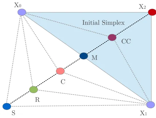
and Mead [66], the gist of the method is as follows. The algorithm uses a so called simplex

consisting ofn+1points for anndimensional function. This consists of the initial starting point

X0 andnother points obtained by shifting each of thendimensions in the starting point by a

predetermined step size. The points in the simplex are sorted from the best to the worst in terms

of function values (in the case of a minimization, the best point would have the lowest function

value). The worst point is replaced by a new point which is computed from the remaining

points (by applying the so called reflection, expansion and contraction operations) in order to

obtain a new simplex. The process is repeated iteratively until a termination criteria is reached.

Details of the procedure are shown in Algorithm 1. Possible choices of replacing the worst

point in Algorithm 1 are shown in Figure 2.1 for a two dimensional function.

X0 _X₂

X1 M

CC

C

R S

[image:37.595.173.447.433.639.2]

Initial Simplex

Figure 2.1: The figure shows the simplex for a 2D function. X0 is the initials starting point.

Assuming that the worst point isX2, the diagram shows possible ways of replacingX2as per

Algorithm 1.

There are several candidates when selecting the termination criteria. Nelder and Mead [66]

(38)

f X X0 x1,x12, . . . ,xn R Output: Xminwhich minimizes f(X)

fori=1tondo ifx_i 6=0then

Xi = [x1,x12, . . . , 1.05xi, . . . ,xn]T else

X_i = [x1,x12, . . . , 0.00025, . . . ,xn]T end if

end for

reorder points such that f(X0)≤ f(X1)≤. . .≤ f(Xn) initial simplex←X0,X1, . . . ,Xn

whiletermination criteria reacheddo

findM =_∑Xi/nfori=0, . . . ,(n−1) find reflected pointR=2M−Xn if f(X0)≤ f(R)< f(Xn−1)then

Xn+1←R

terminate iteration // reflect end if

if f(R)< f(X0)then

find expansion pointS← M+2(M−Xn) if f(S)< f(R)then

Xn+1 ←S

terminate iteration // expand else

Xn+1 ←R

terminate iteration // reflect end if

end if

if f(R)≥ f(Xn−1)then

if f(R)< f(Xn)then

findC←M+ (R−M)/2

iff(C) < f(R) then

Xn+1←C

terminate iteration // contract outside end if

end if

if f(R)≥ f(Xn)then

findCC← M+ (Xn−M)/2 if f(CC)< f(Xn)then

Xn+1←CC

terminate iteration // contract inside end if

end if

end if // shrink

findVi =X0+0.5(Xi−X0)fori∈1, . . . ,n

new simplex←X0,V1, . . . ,Vn find f(Vi)fori∈1, . . . ,n

(39)

estimate for the number of iterations required for convergence as,

I =3.16(n+1)2.11 (2.1)

whereIis the number of iterations required andnis the number of dimensions in the

indepen-dent variable.

The algorithm is a popular direct search method for unconstrained multidimensional

op-timization. For constrained optimization, Nelder and Mead [66] have suggested two ways of

integrating constraints into the optimization. One methods is to modify the function such that

undesired values of the independent variable result in very large function values. The other

method is to transform the independent variable (e.g., use logarithms to exclude negative

val-ues).

2 .

2 Two-view geometry

Epipolar geometry [28] is commonly used to describe the projective geometry of a 3D scene

observed from two views. It is independent of the scene structure, and only depends on the

in-ternal parameters and relative pose of the cameras. As such it is useful in inferring information

about the cameras.

The epipolar geometry can be conveniently represented algebraically using a three by three

matrix of rank two. This matrix is known as theFundamental MatrixF.

When dealing with multi-view geometry, it is convenient to use projective coordinates in Pn_{such that for the Euclidean point}_X

R = (X1,X2, . . . ,Xn)∈Rnthe projective equivalent is

XP =λ(X1,X2, . . . ,Xn, 1)∈Pnwhereλis an arbitrary non-zero scalar. As an aside,

equal-ity in projective coordinates are typically considered only up to a scale factor. For example

(X1,X2, . . . ,Xn, 1) = (2X1, 2X2, . . . , 2Xn, 2) = (λX1,λX2, . . . ,λXn,λ)are all considered

to be projectively equivalent.

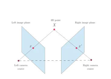
Suppose a point in 3D space X ∈ _P3_{is imaged by the left and right cameras as} _x _∈ _P2

andx0 ∈P2_{respectively, as illustrated in Figure 2.2.}

For noise free measurements of corresponding 2D points x↔ x0, the following condition holds

(40)

X

x

x'

Left camera centre

[image:40.595.93.461.110.373.2]

Right camera centre Left image plane 3D point Right image plane

Figure 2.2: Corresponding points and epipolar geometry

whereFis the fundamental matrix.

F can be computed using a set of known point correspondences x ↔ x0 such that the condition in Equation 2.2 holds. Extensive work has been done on recovering F using point

correspondences including the works by Longuet-Higgins [52], Zhang [91] and Hartley [27].

In most practical situations, the presence of wrong and noisy correspondences can severely

affect the accuracy of the computed F. Therefore, robust estimation techniques based on the

RANSAC approach [20] are typically employed to rule out noisyoutlierswhich do not agree with the F that describes the given data. The point correspondences that satisfy the F are

termedinliers. The workings of a typical RANSAC algorithm are shown in Algorithm 2. In the context of estimating the fundamental matrix, evaluating the modelM in Algorithm 2 would

mean finding anF using a method like the normalized 8 point algorithm as per Hartley [27].

In this case the sampleswould be obtained by picking eight point correspondences. Amongst

other candidates, the distance threshold t can be evaluated using an algebraic distance or a

geometric distance. We use the Sampson distance [77] in our work, which is of the latter type.

Fis said to be degenerate when it fails to uniquely define the epipolar geometry. There are

several situations when the resultingFmay become degenerate. As per Hartley and Zisserman

(41)

Step 2: Find the set of points Si which are within a distance thresholdt of the model; the remaining points inSwill be the set of outliersSo

Step 3:If|Si|>Tthen re-estimateMusing all points inSi and terminate Step 4:If|Si| ≤Tthen repeat from Step 1 up to a maximum ofNtrials

Step 5:Select the largest consensus set obtained so far asSiand re-estimateMwith thisSi

the 3D points are on a ruled quadric or when all the 3D points lie on a plane in 3D. The latter

is of interest to us in Chapter 6 and in such situations it is possible to compute a homography

Hinstead ofF. We may estimate a homographyHsuch that

Hx=x0 (2.3)

Once more it is possible to use robust estimation methods based on the RANSAC approach by

Fischler and Bolles [20] to computeHfrom noisy correspondences. TheSymmetric Transfer Error (STE)[28] is a commonly used distance to measure how much a given point correspon-dence agrees withH. The STE is defined as follows by Hartley and Zisserman [28]. The STE

between point pairsxi ↔ x0i under the homographyHis given as

dSTE(i) =d(xi,H−1xi0)2+d(xi0,Hxi)2 (2.4)

whered(., .)is the Euclidean distance between the inhomogeneous points (inR2) represented

byxi,H−1x0i ∈P2andx0i,Hxi ∈P2. In terms of Algorithm 2, instantiating and re-estimating the model Mwould involve selecting a sets, of four random point correspondences in order

to computeHas per Equation 2.3. In our work, we evaluate the distance thresholdtusing the

STE (Equation 2.4).

However, the degree to which the recovered ForHrepresents the true data when using a

RANSAC based method, is affected by the ratio of inliers to outliers. It is shown by Hartley and

Zisserman [28] that for a given sample size, the number of samples which need to be evaluated

in order to ensure that at least one sample is free from outliers, increases exponentially with

the proportion of outliers (Table 4.3 in Hartley and Zisserman [28]). The requirement, then, is

(42)

Structure from Motion (SfM) algorithms, which estimate the 3Dstructureof the scene and the camera motion given photographs from two or more views, typically require the knowledge of corresponding points across the 2D images. Much work has been done on detecting and

identifying correspondences between multiple views of a 3D scene. However, much of this

work is targeted towards images of non-reflective and well textured objects and scenes.

For example, recent work which has received much attention includesPhoto Tourism[78], which employs the SIFT [53] key point detection and matching algorithm to find point

cor-respondences. This work was originally intended for tourist images commonly found on the

Internet which include outdoor landscapes and historic buildings. As such it does not work

well with images of highly reflective objects containing largely homogeneous regions.

It is worth noting at this point that feature detection and description are two separate tasks

although some algorithms like SIFT [53], SURF [4] and BRISK [48] do both. Other

meth-ods like the key point and edge detector by Harris et al. [26] focus only on the detection aspect. Some common feature descriptors include the use of a histogram of oriented gradients

(HoG) [16] and Phog/Phow descriptors [7] which are commonly used in image classification

and recognition. Similarly work done by Kingsbury [39] shows the utility of a rotation

in-variant feature descriptor based on complex wavelets which can be evaluated on Harris corner

points [26].

Detecting regions covariant with a certain class of transformations can be useful in

find-ing correspondences between views and Mikolajczyket al. [63] have compared some common affine region detectors including MSER, IBR, EBR, Hessian-Affine and Harris-Affine.

De-scriptors for finding wide-baseline correspondences also exist [61, 58, 84]. However, these

methods by themselves are not well suited for images of reflective objects with largely

homo-geneous regions like cars.

Recent work by Linet al. [51] finds correspondences and camera pose using motion coher-ence on scenes which were previously regarded as feature impoverished SfM scenes;

contain-ing largely edge cues but few corners. Their work gives good results on scenes consistcontain-ing of

long edges and few corners such as images of buildings and cupboards. Edge based features

have also been used by Mikolajczyket al. [64] for shape recognition. Good results have been reported from their method on simple smooth shapes like bicycles and tennis rackets, where

edges tend to give strong cues in otherwise poorly textured scenes. Our car images on the other

hand, do not guarantee reliable edges that can be matched across images as edges, since the

(43)

pixel so that descriptors can be read at the desired edge points in the image. Although, dense

implementations of SIFT [53] and SURF [4] exist, we prefer to use the DAISY [84] descriptor

which is faster and also better suited for wide-baseline images. Faster rotation invariant GPU

implementations of the DAISY also exist [19], although we have not used them in our work.

Reflections are not necessarily harmful for the recovery of the epipolar geometry (EPG)

between two images. Work done by Saminathanet al. [81] shows that the epipolar deviations of specularities on convex surfaces which are not highly undulating are usually quite small.

2 .

4 Chapter summary

In this chapter we discussed some background material related to 3D pose estimation, two view

geometry and obtaining reliable point correspondence across photographs from two views. In

the process, an overview of related work was provided. As described in the chapters to follow,

the 3D pose is used to register a 3D CAD model of the vehicle over the photograph. A 2D

projection of the registered 3D CAD model is used as ground truth information when detecting

vehicle damage using the photograph. Our work on 3D model assisted image segmentation

is presented next in Chapter 3, which is used to detect parts of the car in the photograph. We

present a more robust 3D pose estimation method using a novel illumination invariant distance

measure in Chapter 4. Parts of the vehicle in the photograph which were originally not in

the undamaged 3D CAD model can be expected to be vehicle damage. However, based on

this rationale, reflections of the surroundings appearing on the vehicle body can also be

clas-sified as vehicle damage. Therefore, we explore ways to detect such reflections in Chapter 6,

which is based on the work done in Chapter 5 to obtain reliable point correspondences from

(44)

(45)

3 .

1 Introduction

In line with our proposition to use a 3D CAD model to identify parts of the vehicle in a

photograph, we present in this chapter a method to register the 3D model over the photograph

using a gradient based distance measure. In order to identify components of the vehicle in the

photograph, we present a method to segment different parts of a vehicle in the photograph with

the help of the 3D model projection. We address challenging segmentation scenarios where

parts of the car have boundary cues which are difficult for existing segmentation methods. The

work presented in this chapter was published in Jayawardena et al. [37].

Image segmentation is a fundamental problem in computer vision. Most standard

unsuper-vised image segmentation techniques rely on exploiting differences between pixel regions such

as color and texture. Hence, segmenting sub-parts of an object which have similar

character-istics with difficult boundary cues (particularly parts car body with the same color and paint)

can be a challenging task. We propose a method that performs such sub-segmentation with

minimal user interaction and without using any prior training. The only form of additional

input required is the make and model of the vehicle. In our target application of analyzing

vehicle photographs for processing insurance claims, this information is already present in the

insurance policy details, so there is no added burden on the end user to provide extra

infor-mation other than identifying themselves. A result from our method is shown in Figure 3.1

with the car sub-segmented into a collection of parts. These parts include the hood of the car,

windshield, fender, front and back doors/windows.

Sub-segmenting parts of an object which share the same color and texture is very hard with

conventional segmentation methods. However, prior knowledge of the shape of the known

object and its components can be exploited to make this task easier. Based on this rationale we

propose a novelModel Assisted Segmentationmethod for image segmentation.

We propose to register a 3D model of the known object over a given photograph/image in

(46)

Figure 3.1: The figure shows ‘Model Assisted Segmentation’ results for a semi-profile view of a car.

order to initialize the segmentation process. The segmentation is performed over each part of

the object in order to obtain sub-segments from the image. A major contribution of this chapter

is a novel gradient based distance measure, which is used to estimate the full 3D pose of the

object in the given image. The projected parts of the 3D model may not perfectly match the

corresponding parts in the photograph due to dents in a damaged vehicle or inaccuracies in the

3D model. Therefore, a level-set [50] based segmentation method is initialized using initial

contour information obtained by projecting parts of the 3D model at this 3D pose. We focus

our work on sub-segmentation of known car images. Cars present a difficult segmentation task

due to the highly reflective surfaces in the car body. Our method can be adapted to work on

any other object as well.

The remainder of this chapter is organized as follows. We describe the method used to

estimate the 3D pose of the object in Section 3.2. The contour based image segmentation

approach is described next in Section 3.3. This is followed by results on real photographs

which are benchmarked against state of the art methods in Section 3.4.

3 .

2

3 D model registration

We describe the use of a featureless gradient based distance measure which is used to register

the 3D model over the 2D photo. Our method uses triangulated 3D CAD models with a large

number of polygons (including 3D models obtained from laser scans) and utilizes image

gra-dients of the 3D model surface normals rather than considering simple edge segments as done

by Kollnig and Nagel [42].

3.2.1 Gradient based distance measure

We define a gradient based distance measure that has a minimum at the correct 3D poseθ0 ∈

(47)

d=3ifWis an RGB image) having elementsW(u,v)∈ IR . We define thepnorm ‘gradient magnitude’ matrix ofW as

||∇W(u,v)||k

k :=∑di=1

|∂Wi(u,v)

∂u |

k₊_|∂Wi(u,v)

∂v |

k _(3.1)

Based on this we have the gradient magnitude matrixGI for a 2D photo/imageIas

GI(u,v) =||∇I(u,v)||k_k (3.2)

Letφ(x,y,z,θ) = φx φyφz

T

∈ IR3be the unit surface normal at the 3D pointp= (x,y,z)

of the 3D model at poseθ. The model is rendered with the surface normal components values

φx,φyandφzused as RGB color values in the OpenGL renderer to obtain the projected surface

normal component matrixΦsuch thatΦ(u,v,θ)∈ IR3has surface normal component values at the 2D point(u,v)in the projected image. Based on this we have the gradient normal matrix for the surface normal components as

GN(θ)(u,v) =||∇Φ(u,v,θ)||k_k (3.3)

We define the distance measureLg(θ)for a given poseθas

Lg(θ):=1−(corr(GN(θ),GI))2∈ [0, 1] (3.4)

wherecorr(GN(θ),GI)is the Pearson’s product-moment correlation coefficient [74] between

the matrix elements of GN(θ)and GI. This distance measure has a convenient property of

ranging between0and1. Lower distance measure values imply a better 3D pose.

3.2.2 Visualisation

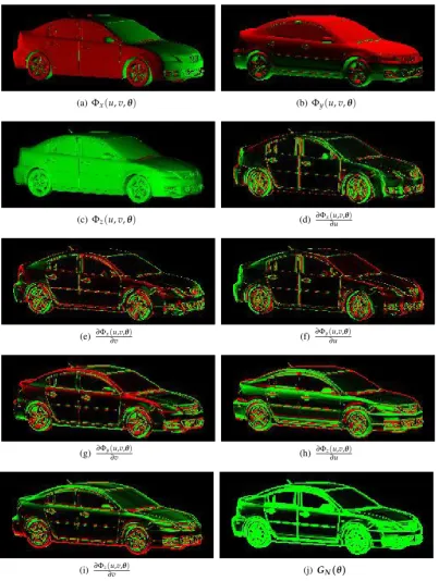
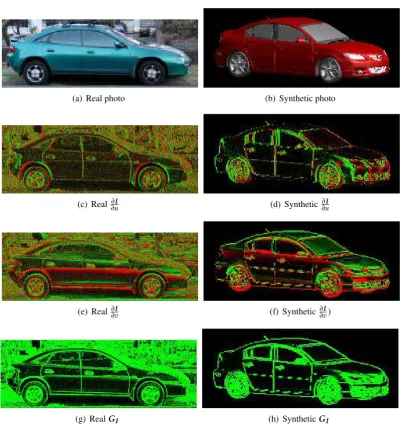
We illustrate intermediate steps of the distance measure calculation for a 3D model of a Mazda

3 car. The surface normal componentsΦx(u,v,θ)Φy(u,v,θ)andΦz(u,v,θ)are shown in Figure 3.2(a-c). Their image gradients are shown in Figure 3.2(d-i) and the resultingGN(θ)

matrix image is shown in Figure 3.2(j). Similarly intermediate steps in the calculation of GI

are show in Figure 3.3 for a real photograph and a synthetic photo. We show overlaid images

(48)

real and synthetic photo. The synthetic photograph was made by rendering the Mazda 3 model

at a known poseθ. The real photograph is of a Mazda Astina. An accurate 3D model obtain

from a laser scan is used with this real photograph. The model projections steps for for the

Astina are not included but are similar to what is shown in Figure 3.2(a).

The correlation will be highest in Equation 3.4 when the 3D model is projected with pose

parametersθ0that match the object in the photographF, as this has the best overlap. Therefore

the distance measure will be lowest at the correct pose parametersθ0, for values ofθreasonably

close toθ0. We see this in the distance measure landscapes in Figure 3.5.

3.2.3 Gaussian smoothing

We apply Gaussian smoothing on the photograph and rendered surface normal component

images before calculatingGI(Equation 3.2) and GN(θ)(Equation 3.3). This is done by

con-volving with a 2D Gaussian kernel followed by down-sampling [22]. This makes the distance

measure landscape less steep and noisy, thus making it easier to optimize. However, the global

optimum tends to deviate slightly from the correct pose at high levels of Gaussian smoothing.

Compare the 1D distance measure landscapes shown in Figure 3.5 for different levels of

Gaus-sian smoothingn. Therefore, we hierarchically perform a series of optimizations starting from

the highest level of smoothing, using the optimum found at levelnas the initialization for level

n−1, recursively.

3.2.4 Choosing the norm p

We have a choice when selecting the norm for Equations 3.2 and 3.3. Having tested both1

-norm and2-norm cases we have found the1-norm to be less noisy (as shown in Figure 3.5)

and hence easier to optimize.

3.2.5 Representation of the pose

Careful selection of pose parameters can aid the optimizer when finding the best pose. The pose

of a generic object may be represented by translations along the X,Y and Z axes and a suitable

rotation representation. According to Lepetit and Fua [47], an Euler angle based rotation

representation may give rise to ill-conditioned optimization problems due to a situation known

as the Gimbal Lock, which occurs when two of the three rotations axes align and rotations around the third axis ceases to have any effect. A quaternion or exponential map rotation

representation may be used to avoid this problem. Since we work with vehicles, the following

(49)

(a)Φx(u,v,θ) (b)Φy(u,v,θ)

(c)Φz(u,v,θ) (d) ∂Φx(_∂u_u,v,θ)

(e) ∂Φx(u,v,θ)

∂v (f)

∂Φy(u,v,θ)

∂u

(g) ∂Φy(u,v,θ)

∂v (h)

∂Φz(u,v,θ) ∂u

(i) ∂Φz(u,v,θ)

[image:49.595.119.523.114.649.2]

∂v (j) GN(θ)

Figure 3.2: The visualizations showsGN(θ)for a Mazda 3 3D CAD model in (j). The x,y and

z component matrices of the surface normal vector are shown in (a)-(c). Their image gradients are shown in (d)-(i). The resultingGN(θ)matrix is shown in (j). No Gaussian smoothing has

been applied. Color representation: green=positive, black=zero and red=negative. We use a horizontalxaxis pointing left to right, verticalyaxis and pointing top to bottom and anzaxis

(50)

(a) Real photo (b) Synthetic photo

(c) Real ∂I

∂u (d) Synthetic

∂I

∂u

(e) Real ∂I

∂v (f) Synthetic∂

I

∂v)

[image:50.595.77.483.177.602.2]

(g) RealGI (h) SyntheticGI

Figure 3.3: Intermediate steps in calculatingGIfor a real (column 1) and synthetic photograph

(column 2). The synthetic photograph was made by projecting the 3D model. Image gradients (rows 2 and 3) andGI (row 4) are shown. Colour representation: green=positive, black=zero

(51)

(a) Real (b) n=0 (c) n=2

(d) Synthetic (e) n=0 (f) n=2

Figure 3.4: Overlaid images of GI andGN(θ)for a real photograph (row 1) and a synthetic photograph (row 2) obtained by rendering a 3D model are shown. The first column shows the photographs I. The overlaid images ofGI andGN(θ)with no Gaussian smoothing (column

2) and 2 levels of Gaussian smoothing (column 3) are shown. The photograph is in the green channel and 3D model is in the red channel, with yellow showing overlapping regions.

0.975 0.98 0.985 0.99 0.995 1

-15 -10 -5 0 5 10 15

Los

s V

al

ue

Percentage shift in x direction from known pose n = 0 n = 1 n = 2

(a) 2-norm

0.75 0.8 0.85 0.9 0.95 1

-15 -10 -5 0 5 10 15

Los

s V

al

ue

Percentage shift in x direction from known pose n = 0 n = 1 n = 2

(b) 1-norm

Figure 3.5: We compare1-norm and2-norm gradient based distance measure landscapes ob-tained by shifting the 3D model along the x direction from a known 3D pose. The horizontal axis shows the percentage deviation along the x axis. This is obtained by varyingµx in the pose representation give in Section 3.2.5. The numbers in the legend show the level of Gaus-sian smoothing napplied on the gradient images before calculating the distance measure in Equation 3.4. We note that the1-norm distance measure is less noisy compared to the2-norm distance measure. The actual distance measure is seven dimensional and graphs of the other

(52)

Figure 3.6: The pose representation θortho used for 3D car models. We use the rear wheel centerµ, the vector between the wheel centersδand unit vectorψin the direction of the rear

wheel axle.

representation is consistent with pose representation used in the rough pose estimation method

of Hutter and Brewer [33], which we use for our work.

θortho:= µx,µy,δx,δy,ψx,ψy

(3.5)

In this representation, µ = (µx,µy) is the visible rear wheel center of the car in the 2D projection. δ = (δx,δy)is the vector between corresponding rear and front wheel centers of the car in the 2D projection. The 2D image is a projection of the 3D model on to the XY

plane. ψ = ψx,ψy,ψz

is a unit vector in the direction of the rear wheel axle of the 3D

car model. Therefore,ψz = −

√

1−ψ2_x−ψ2_yand need not be explicitly included in the pose

representationθ. This representation is illustrated in Figure 3.6. This pose is converted to

OpenGL translation, scale and rotation as per Hutter and Brewer [33] to transform and project

the 3D model. As we directly optimize Equation 4.5 with respect to θ(Section 4.5) explicit

knowledge of intrinsic camera parameters etc,. are not required.

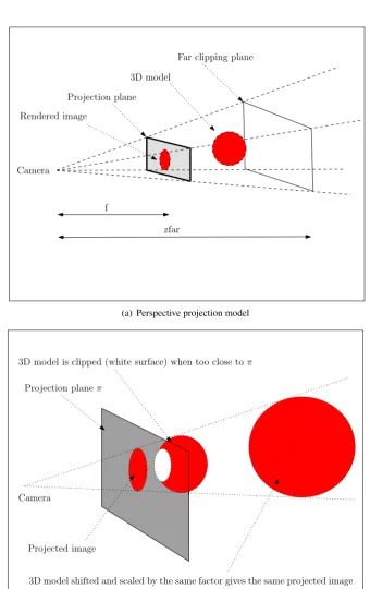
3.2.5.1 Perspective projection

We extend the pose estimation to handle perspective projection as follows. The 3D model is

rendered using the OpenGL perspective projection model. The degree of perspective distortion

can be changed by varying the focal length parameterf (Figure 3.7(a)) in the OpenGL frustum.

Therefore, we include the parameter f as a pose parameter during the optimization. We now

have the following perspective pose representation (with seven degrees of freedom) instead of

the previous representation given in Equation 3.5.

θpersp:= µx,µy,δx,δy,ψx,ψy,f