Quantum discord, EPR steering and Bell-type correlations for secure CV quantum communications

Quantum Discord, EPR Steering

and Bell-type Correlations for

Secure CV Quantum

Communications

Sara Hosseini

A thesis submitted for the degree of

Doctor of Philosophy of the

The Australian National University

Declaration

This thesis is an account of research undertaken between February 2012 and Febru-ary 2016 at the Department of Quantum Sciences, The Research School of Physics and Engineeringat theAustralian National University, in Canberra, Australia.

Except where acknowledged in the customary manner, the material presented in this thesis is, to the best of my knowledge, original and has not been submitted in whole or part for a degree in any university.

Sara Hosseini 15 February 2017

Acknowledgments

My PhD at Quantum Optics group led by Prof. Ping Koy Lam at the Australian National University was a great opportunity for me to learn and work on one the advanced field of science and technology. This was a challenging, beautiful and ex-tremely fruitful journey for me that I will remember and cherish through all my life. Many people played an important role during this journey helping me to accomplish it that I would like to thank them here.

At first, I would like to sincerely thank Prof. Ping Koy Lam, the head of my super-visory panel and head of the group. Ping Koy has always been very kind, positive, encouraging and supportive to me, wanting the best for me and for all the group members. The level of support that he provided and the kindness that he showed to me, were more than what I expected. Without his moral, scientific and financial supports this would not be possible for me to accomplish this program.

Secondly I would like to thank my parents Akhtar Mirza and Mir. Mohammad Hos-seini who have loved me unconditionally and supported me through all my life. This happened due to their encouragement and their tolerance and scarifice during these four years while I was far from them in order to peruse my passions. I also would like to thank my two sisters; Narjis Hosseini and Mona Hosseini, the true friends and supporters in my life, whose love warms my heart in the most difficult situa-tions. Mona’s two years presence in Canberra specially made my PhD much more enjoyable. Those years surely remain one of the most memorable time in our lives. In addition, I would like to thank Thomas Symul, my very kind supervisor. It was a great opportunity for me to know Thomas and work under his supervision. He has always been very gentle and supportive. I also would like to thank Ben Buchler for his kind and positive attitude towards me.

I sincerely thank Syed M Assad, the kindest and the most intelligent person I know, and Jiri Janousek, the hero in the lab. From the beginning of my PhD both Assad and Jiri provided incredible level of support to me. I deeply enjoyed working and discussing scientific issues with them.

I also would like to thank all my colleagues and the post-doctoral fellows in our group, who I have had the chance to work with, for their productive collaboration and kind support including Jing Yan Haw, Seiji Armstrong, Oliver Thearle, Geng Jiao, and the ones who I have not had the chance to collaborate, but I extremely enjoyed their company and friendship including Alexandre Brieussel, Giovanni Guc-cione, Pierre Vernaz-Gris, Zhao Jie, Geoff Campbell, Jesse Everett, Shen Yong and Daniel Higginbottom. Besides, I would like to thank the theorists that I have collab-orated with; Prof. Timothy C Ralph, Prof. Howard M Wiseman, Nathan Walk and Saleh Rahimi-Keshari.

students.

My sincere thanks to my best friends Farzaneh Kordbacheh and Mona Golestanfar for supporting me like a family members through all the years of my PhD.

Abstract

Quantum states can be correlated in ways beyond what is possible for classical states. These correlations are considered as the main resource for quantum compu-tation and communication tasks. In this thesis, I present my studies on the different forms of Quantum Correlations known as "Quantum Discord", "Einstein-Podolsky-Rosen(EPR) Steering" and "Bel-type correlations" in the continuous-variable quantum states and investigate their practical applications for the secure quantum communi-cation.

While previously quantum entanglement was considered as the only form of quan-tum correlation, in the recent years a notion known as quanquan-tum discord which cap-tures extra quantum correlations beyond entanglement was introduced by Ollivier and Zurek. This sort of non-classicality that can exist even in separable states, has raised so much aspiration for the potential applications, as they are less fragile than the entangled states. Therefore, of especial interest is to know if a bipartite quan-tum state is discordant or not. In this thesis I will describe the simple and efficient experimental technique that we have introduced and experimentally implemented to verify quantum discord in unknown Gaussian states and a certain class of non-Gaussian states. According to our method, the peak separation between the marginal distributions of one subsystem conditioned on two different outcomes of homodyne measurement conducted on the other subsystem is an indication of nonzero quan-tum discord. We implemented this method experimentally by preparing bipartite Gaussian and non-Gaussian states and proved nonzero quantum discord in all the prepared states.

Though quantum key distribution has become a mature technology, the possibil-ity of hacking the devices used in the quantum communications has motivated the scientists to develop the schemes where one or non of the devices used by the com-municating parties need to be trusted. Quantum correlations are the key to de-velop these schemes. Particularly, EPR steering is connected to the one-sided-device-independent quantum key distribution in which devices of one party are solely trusted and Bell-type correlations to the fully device-independent quantum key dis-tribution where non of the apparatuses of the communicating parties is trusted. Here, I will present the result of our theoretical and experimental research to de-velop one-sided-device-independent quantum key distribution in continuous vari-ables. We identify all Gaussian protocols that can in principle be one-sided-device-independent. This consists of 6 protocols out of 16 possible Gaussian protocols, which surprisingly includes the protocol that applies only coherent states. We ex-perimentally implemented both the entanglement-based and coherent state proto-cols and manifested their loss tolerance. Our results open the door for the practical secure quantum communications, asserting the link between the EPR-steering and

one-sided-device-independence.

Contents

Declaration ii

Acknowledgments vii

Abstract ix

1 Introduction 1

1.1 Publications (Article and Conference paper) . . . 3

1.2 Thesis Outline . . . 3

2 Theoretical Background 7 2.1 Quantum Optics . . . 7

2.2 Quantisation of the electromagnetic field . . . 7

2.3 Quadratures of the electromagnetic field . . . 8

2.4 Quantum States of Light . . . 9

2.4.1 Quadrature States . . . 10

2.4.2 Fock States . . . 10

2.4.3 Coherent States . . . 11

2.4.4 Squeezed States . . . 12

2.4.5 Thermal States . . . 13

2.5 Wigner Function . . . 14

2.6 Gaussian States . . . 15

2.6.1 Symplectic Transformations and the Gaussian Unitaries . . . 16

2.6.2 Williamson Theorem and Symplectic Spectrum . . . 16

2.6.3 Standard form of two-Mode Gaussian states . . . 17

2.7 Quantum Measurements . . . 17

2.7.1 Positive-Operator-Value-Measurement (POVM) . . . 18

2.8 Measurement in Quantum Optics . . . 18

2.8.1 Quadrature Measurement . . . 19

2.8.2 Simultaneous Measurement of Two Quadratures . . . 20

2.9 Phase and Amplitude Modulation . . . 20

2.9.1 Phase Modulation . . . 21

2.9.2 Amplitude Modulation . . . 22

2.10 Information Theory and Entropy . . . 22

2.10.1 Shannon Entropy . . . 22

2.10.2 Relative Entropy . . . 23

2.10.3 Shannon Entropy of Continuous Random Variable . . . 23

2.10.4 Joint Entropy . . . 23

2.10.5 Conditional Entropy . . . 23

2.10.6 Mutual Information . . . 24

2.10.7 von Neumann Entropy . . . 24

2.10.8 Quantum Mutual Information and Conditional Entropy . . . 25

2.10.9 Holevo Bound . . . 25

2.11 Quantum Correlations . . . 26

2.11.1 Entanglement and non-locality . . . 26

2.11.2 Entanglement Criteria for Pure Bipartite States . . . 26

2.11.3 Entanglement Criteria for Mixed States . . . 27

2.11.4 Duan Inseparability Criterion . . . 28

2.11.5 EPR Paradox Criterion . . . 28

2.11.6 Quantum Discord . . . 29

2.12 Summary . . . 29

3 Experimental Verification of Quantum Discord in Continuous-Variable States 31 3.1 Introduction . . . 31

3.2 Definition of Quantum Discord . . . 33

3.3 Gaussian Quantum Discord . . . 33

3.4 Verification of Quantum Discord in General . . . 34

3.5 Experimental Method to Verify Quantum Discord in CV Systems . . . . 35

3.6 Theoretical Development of Verification of Quantum Discord in Continuous-Variables . . . 35

3.6.1 Theory: Gaussian States . . . 35

3.6.2 Theory: Non Gaussian States . . . 36

3.7 Experimental Implementation of Verification of Quantum Discord in Continuous-Variables . . . 37

3.7.1 Electro-Optic Modulators (EOM) . . . 37

3.7.2 Source Laser . . . 38

3.7.3 Seed Beam Preparation . . . 39

3.7.4 Producing a vacuum state with Gaussian distributed noise . . . 41

3.7.5 Experimental Implementation of Verification of Quantum Dis-cord in Gaussian States . . . 41

3.7.6 Experimental Implementation of non-Gaussian State . . . 44

3.8 Summary . . . 47

4 Secure Quantum Communication 49 4.1 Introduction . . . 49

4.2 A Generic QKD Protocol . . . 50

4.3 Device Independent Quantum Key Distribution . . . 51

4.3.1 Usual QKD protocols are not secure in the device-independent scenario . . . 52

4.3.2 How can DI-QKD possibly be secure? . . . 52

Contents xiii

4.4 Measurement-Device-Independent Quantum Key Distribution . . . 56

4.5 One-sided Device-Independent Quantum Key Distribution . . . 57

4.6 Summary . . . 58

5 Theoretical Development of 1SDI-QKD 61 5.1 Introduction . . . 61

5.2 Uncertainty Relations . . . 62

5.3 Quantum Cryptography in Continuous-Variable Regime . . . 63

5.3.1 Virtual Entanglement . . . 64

5.4 CV-QKD using entropic uncertainty relations . . . 65

5.5 Security proof with imperfect reconciliation efficiency . . . 68

5.6 One-sided device-independent CVQKD . . . 69

5.6.1 EPR Steering . . . 70

5.6.2 One-sided device-independent CV-QKD protocols and their con-nection to EPR steering . . . 70

5.7 Summary . . . 74

6 Experimental Implementation of 1SDI-QKD Protocols in EB Scheme 75 6.1 Introduction . . . 75

6.2 Experimental Setup . . . 75

6.3 Optical Parametric Amplifier . . . 76

6.3.1 Locking loops of the OPAs . . . 79

6.3.2 Alignment of the OPAs . . . 79

6.3.3 Characterization of the OPAs . . . 81

6.4 Entanglement Generation . . . 81

6.5 Control System and Data Acquisition . . . 83

6.6 Experimental Results . . . 84

6.7 Computer Modeling . . . 85

6.8 Summary . . . 87

7 Experimental Implementation of 1SDI-QKD Protocols in P&M scheme 91 7.1 Introduction . . . 91

7.2 Experimental Implementation of P&M Scheme . . . 91

7.2.1 Calibration of function generator outputs . . . 92

7.3 Control System and Data Acquisition . . . 94

7.4 Results . . . 94

7.5 Error Estimation . . . 95

7.6 Computer Modeling . . . 98

7.7 Summary . . . 100

8 Bell-like Correlations for Continuous-Variables 101 8.1 Introduction . . . 101

8.2 Mathematical Description of Bell’s Inequality . . . 101

8.3 CHSH Inequality . . . 103

8.5 Computer Modelling of two systems showing Bell type correlation in CV regime . . . 107 8.6 Summary . . . 111

9 Conclusion 113

9.1 Future Work . . . 114

List of Figures

1.1 Structure of this thesis. . . 6

2.1 Phase-space representation of a coherent state. . . 12

2.2 Phase-space representation of a squeezed state. . . 12

2.3 Schematic diagram of a balanced homodyne detection. . . 19

2.4 Schematic diagram of heterodyne (dual-homodyne) detection. . . 21

2.5 Venn diagram. . . 24

3.1 Schematic diagram of a mode cleaning ring cavity and the feed back control loop. . . 40

3.2 Vacuum state with Gaussian distributed noise. . . 41

3.3 (a) Schematic diagram of the experimental setup. (b) The uncondi-tioned (left) and condiuncondi-tioned (right) probability distributions of the bipartite Gaussian state with discord. . . 42

3.4 Variation of peak separations of marginal distributions conditioned on two different homodyne outcomes, versus modulation depth. (b) shows the zoom-in for small modulation depth. . . 45

3.5 Schematic diagram of the modulation and demodulation arrangements used in preparation of the non-Gaussian states. . . 46

3.6 Unconditional and conditional probability distributions of two differ-ent outcomes of the non-Gaussian states. . . 48

4.1 Schematic diagram of Standard QKD, DI-QKD, 1SDI-QKD and MDI-QKD . . . 59

5.1 Virtual entanglement. . . 65

5.2 Schematic diagram of steering task when Alice is affecting Bob’s state. . 71

5.3 Gaussian protocols which can potentially be 1SDI. . . 72

5.4 Schematic diagram of all the experimentally realised 1sDI protocols. . . 73

6.1 Schematic diagram of the general form of the experimental setup using an entangled source. . . 77

6.2 Schematic diagram of the three experimental setups using an entan-gled source. . . 78

6.3 Schematic diagram of the optical parametric amplifier bow-tie cavity. . 79

6.4 Schematic diagram of the Optical Parametric Amplifier and the feed back control loops. . . 80

6.5 Squeezing and anti-squeezing values of OPA1 and OPA2 measured at 3 MHz, as a function of the pump power. . . 81 6.6 Generation of two mode EPR state. . . 82 6.7 Schematic diagram of the model used to predict the pure squeezing. . . 83 6.8 Key rates versus the applied loss in dB scale for (a) DR and RR

proto-cols with EB source and homodyne-homodyne detections. . . 86 6.9 Schematic diagram of the modelling of the 1SDI-QKD experiment

us-ing entangled source and homodyne-homodyne measurements. . . 88 6.10 Predicted improvement of secure communication for the EB protocols. . 89

7.1 Schematic diagram of experimental setup implementing P&M scheme. 93 7.2 Simple diagram of P&M scheme showing only one quadrature. . . 93 7.3 Schematic diagram of the homodyne lock utilized in P&M experiment. 95 7.4 Variation of key rates versus effective modulation squeezing parameter

for 5 different values of the applied loss. . . 96 7.5 Key rates versus loss in dB scale for P&M coherent state DR protocol. . 97 7.6 Comparison of key rates resulted from optimum modulation variances

versus the applied loss in dB scale for our experimental system and an ideal system with out any imperfections. . . 99

8.1 Schematic diagram of a two channel CHSH Bell experiment. . . 104 8.2 Schematic diagram of a quantum optical system that can be used to

demonstrate the violation of Bell’s inequality. . . 105 8.3 Schematic diagram of system S1 using four squeezing sources

pro-posed in [1]. . . 107 8.4 Schematic diagram of system S2 using two squeezing sources

pro-posed in ref [2]. . . 108 8.5 Plots showing the maximum violation of Bell’s inequality (Bmax) as a

List of Tables

2.1 Classification of light based on the photon statistics [31] . . . 13

Chapter1

Introduction

The peculiar nature of quantum entanglement was first indicated by Einstein, Podol-sky and Rosen (EPR) in their famous seminal paper in 1935 [3]. This paradox which considers two main aspects of quantum mechanics; entanglement and uncertainty principle [4], was proposed to prove that the quantum mechanics was not complete in that current formalism and should includelocal hidden variabletheories. Their con-troversial proposal raised so many debates in physics until 1964 when John Stewart Bell quantified local realistic theories through his famous inequality [5]. The viola-tion of Bell’s inequality guarantees that a pair of particles are genuinely entangled and their correlation cannot be described by any form of local theories.

The concept of quantum entanglement, later received tremendous amount of atten-tion as the essential resource for quantum informaatten-tion tasks, including"Quantum Key Distribution (QKD)"[6, 7] which appeared by the proposals of Bennett and Brassard’s [8] in 1984, and Ekert’s [9] in 1991. This cryptographic technique which rely solely on the laws of quantum mechanics, promises unbreakable security, what human beings has endeavoured to achieve during the whole history!

Though the field of Quantum Key Distribution developed rapidly with so many suc-cess stories [10, 11, 12], it is soon realized that the real-life implementation might differ from the theoretical predictions. This means that unbreakable security will no longer be guaranteed, unless less or more realistic assumptions about the devices are considered. In order to tackle this problem, protocols with least amount of assump-tions on devices were developed, now known as Device Independent QKD (DI-QKD) [13, 14]. However, DI-QKD requires the strong form of quantum non-locality (Bell’s non-locality) to prove the unconditional security. The fact that the violation of the de-tection loop-hole free Bell test [15, 16] itself is a challenge to the experimental physics, makes a field implementation of the DI-QKD protocols currently troublesome. One may think that less stringent form of quantum correlation may be advantageous, which is indeed true. An asymmetric form of quantum correlation known as EPR-steering, which was first proposed by Schrödinger in 1935 as a generalization of the EPR paradox [17] is linked to the new kind of quantum security, so called one-sided device independent QKD (1SDI-QKD) [18, 19]. In these protocols only the appara-tuses of one of the communicating parties are reliable. In addition, the link between entanglement and uncertainty relations which was first mentioned by EPR has been quantified by Berta et al. in ref [20] by employing entropic version of uncertainty

relations [21, 22, 23, 24, 25]. This provided new means for cryptographers, which hand in hand with the concept of EPR-steering make the development of 1SDI-QKD protocols possible. The requirements to satisfy the 1SDI-QKD protocols are less strict than DI-QKD protocols which makes them an interesting candidate for practical ap-plications.

One of the main focus of my thesis is the advancement of 1SDI-QKD protocols in continuous-variables which are presented in Chapters 5, 6 and 7. By using en-tropic version of uncertainty relations in continuous variables [26, 27, 28] , we lower bounded the asymptotic secret key rate of all the 16 possible Gaussian OKD proto-cols, and showed that only 6 of them can manifest one-sided device-independence. We implemented 5 of these 6 protocols experimentally and demonstrated that the best system using entangled source and homodyne-homodyne measurements can tolerate an applied loss of up to 1.5 dB. Surprisingly, we implemented a protocol that utilizes only coherent states as the source, and showed that it can tolerate an applied loss of up to 0.6 dB. This was the first demonstration of 1SDI-CVQKD using coherent states. The ease and the low price of producing coherent states compared to the entangled states, make these sources a very interesting candidate for short-range networks. I also developed a detailed computer modelling to understand our experimental setups and the potential for further improvements. Our theoretical and experimental research, further strengthen the link between the 1SDI-QKD and EPR-streeing.

Though entanglement is regarded as the essential tool for quantum computation and communication, the research during the last decade has proven that it is not the unique form of quantum correlation. A form of quantum correlation which can exist even in the separable states was introduced and characterized by Henderson and Vedral in 2001 [29] and separately by Ollivier and Zurek in 2001 [30]. Ollivier and Zurek named it "Quantum Discord". This new form of quantum correlation which is more robust than entanglement has evoked large number of attention during the last decade, promising new asset for quantum information tasks. Due to the increas-ing interest in quantum discord and the difficulty of calculatincreas-ing it for an unknown quantum state, it is important to find a method to verify quantum discord in an unknown quantum state. We have introduced and implemented experimentally a straightforward method to verify quantum discord in unknown Gaussian states and non-Gaussian states that are prepared by overlapping a vacuum state and a statistical mixture of coherent states on a 50:50 beamsplitter. In Chapter 3, I present a through discussion on quantum discord and our discord verification method as well as the implementation and the results of our experimental survey .

§1.1 Publications (Article and Conference paper) 3

1

.

1

Publications (Article and Conference paper)

A large part of the material presented in the following chapters are published in the peer-review journals or presented in conferences. The list of publications and conference proceedings are as follows:

• N. Walk, S. Hosseini, J. Geng, O. Thearle, J. Y. Haw, S. Armstrong, S. M. Assad, J. Janousek, T. C. Ralph, T. Symul, H. M. Wiseman and P. K. Lam. "Experimental Demonstration of Gaussian Protocols for one-sided device independent quantum key distribution", Optica3(6), 634-642 (2016).

• S. Hosseini, S. Rahimi-Keshari, J. Y. Haw, S. M. Assad, H. Chrzanowski, J. Janousek, T. Symul, T. C. Ralph and P. K. Lam, "Experimental Verification of Quantum Discord in Continuous-Variable States", J. Phys. B: At. Mol. Opt. Phys. 47, 025503 (2014).

• H. Chrzanowski, N. Walk, S. M. Assad, J. Janousek, S. Hosseini, T. C. Ralph, T. Symul and P. K. Lam, "Measurement-based Noiseless Linear Amplification for Quantum Communication", Nature Photonics8, 333-338 (2014).

• S. Hosseini, S. Rahimi-Keshari, J. Y. Haw, A. M. Syed, H. M. Chrzanowski, J. Janousek, T. Symul, T. Ralph, P. K. Lam, M. Gu, K. Modi, and V. Vedral, "Ex-perimental Verification of Quantum Discord and Operational Significance of Discord Consumption", in CLEO: 2014, OSA Technical Digest (online) (Optical Society of America, 2014), paper FTh3A.6.

• H. Chrzanowski, N. Walk, O. Thearle, S. M. Assad, J. Janousek, S. Hosseini, T. C. Ralph, T. Symul, P. K. Lam, "Measurement-based Linear Amplification for quantum communication", Quantum and Nonlinear Optics III (2014).

• J. Janousek , H. Chrzanowski , S. Hosseini, S. M Assad, T. Symul, N. Walk, T. C Ralph, P. K. Lam,"Virtual Noiseless Amplification", CLEO/Europe-IQEC 2013 Conference on Lasers and Electro-Optics-Int Quantum Electronics Conference (2013) 1.

1

.

2

Thesis Outline

Chapter 2: Theoretical Background.

In this chapter I provide the theoretical background on quantum optics which are necessary to understand the rest of the thesis. This includes quantisation of the electromagnetic field, quantum states of light, Wigner function and Gaus-sian states, quantum measurements, phase and amplitude modulation, classical and quantum information theory and quantum correlations.

Chapter 3: Experimental Verification of Quantum Discord in CV States.

In this chapter I review the concept of Quantum Discord, Gaussian quantum discord, and a general method to verify quantum discord. Then I present the experimental method that we proposed and implemented to verify quantum discord in continuous-variable (CV) states. I describe our theoretical develop-ment of the technique as well as the details of our experidevelop-mental impledevelop-mentation including the description on different parts of our setup and present our results.

Chapter 4: Secure Quantum Communication.

In this chapter I looked at "Quantum Key Distribution" and the standard form of it. Then I introduce the proposed methods to close the gaps between the-ory and practical implementation of QKD protocols. These methods include "Device-Independent QKD", "Measurement-Device-Independent QKD" and "One-sided Device-Independent QKD". I reviewed large number of researches that developed these techniques.

Chapter 5: Theoretical Development of 1SDI-QKD Gaussian Protocols.

In this chapter I discuss the one-sided device-independent quantum key dis-tribution and its connection to EPR steering, I present our theoretical analy-sis to derive the key rates for 1SDI-QKD protocols using Gaussian states and measurements. I elaborate all the concepts that help to understand our theoreti-cal development; including entropic uncertainty relations, virtual entanglement and EPR-steering.

Chapter 6: Experimental Implementation of 1SDI-QKD Protocols in EB Scheme. In this chapter I detail our experimental implementation of 1SDI-QKD proto-cols using an entangled source. I describe the technique and equipments that we used to generate amplitude squeezed light and entanglement and explain our control system and data aqcusition. I elucidate our experimental results, error estimation and the computer model that I developed to simulate our ex-periments.

§1.2 Thesis Outline 5

Chapter 8: Bell-like Correlations for Continuous-Variables.

This chapter is a brief report on our research on the possibility of the experi-mental demonstration of Bell-like correlation for continuous variables. Due to the progress of CV regime in quantum information, it is of particular interest to perform a Bell test using continuous sources and detections. This experiment is based on the proposal of ref [1, 2]. I conducted a computer simulations to understand these experimental setups and investigate is Bell’s inequality can be violated using continuous variables. I present the details of my modelling and its result in this chapter.

Chapter 9: Conclusion.

Bell-like Correlations for Continuous-Variables Theoretical Background

Experimental Verification of Quantum Discord in CV States

Secure Quantum Communication

Theoretical Development of 1SDI-QKD Gaussian Protocols

Experimental Implementation of 1SDI-QKD Protocols in EB Scheme

Experimental Implementation of 1SDI-QKD Protocols in P&M Scheme

Conclusion Introduction

Chapter2

Theoretical Background

2

.

1

Quantum Optics

Quantum optics is a field in which the optical phenomena can only be described em-ploying the laws of quantum mechanics. The pioneering ideas of quantum theories of light started from 1901 with Planck’s description of black-body radiation as dis-crete energy packets called quanta, followed up in 1905 by Einstein’s explanation of the photoelectric effect applying Planck’s hypothesis. The precise theory of quantum optics appeared after the birth of quantum mechanics with Dirac’s seminal paper on quantum theory of radiation in 1927. However, looking for quantum effects as-sociated with optical field was not important till 1963 after Glauber described new states of light with different statistical properties from classical light. Non-classical properties of light like photon antibunching were demonstrated experimentally by Kimble, Dagenais and Mandel in 1977 and squeezing in 1985 by Slusher et al. These led to the birth of the new and fast growing field of Quantum Opticswith so many applications and other disciplines being involved with it like quantum information processing [31]. In this chapter I will review some of the key concepts of quantum optics and quantum information theory which will be used through out the entire thesis.

2

.

2

Quantisation of the electromagnetic field

Quantum description of light requires quantisation of the electromagnetic field. In order to quantize the electromagnetic field we can start from source free Maxwell equations [38]:

∇ · B=0, (2.1)

∇ ×E=−∂B

∂t, (2.2)

∇ · D=0, (2.3)

∇ ×H= ∂D

∂t , (2.4)

Where B = µ0H, D = ε0E, µ0 is the magnetic permeability and ε0 is the electric

permittivity of free space. Considering the Coulomb gauge,(∇ · A=0), electric and magnetic fields can be derived from a vector potentialA(r,t)as follows [38]:

B=∇ ×A, (2.5)

E=−∂A

∂t , (2.6)

Considering the equations (2.5) and (2.4), it is seen that the vector potential Aobeys the wave equation. Hence, the vector potential can be described as follows [38]:

A(r,t) =

∑

k

( ¯h 2ω_kε0

)1/2[akuk(r)e−iωkt+a†ku∗k(r)eiωkt] (2.7)

Where ¯his the Planck’s constant, uk(r)corresponds to the set of vector mode

func-tions with frequency ω_k which satisfy the wave equation. This leads to the corre-sponding electric field as follows [38]:

E(r,t) =i

∑

k

(¯hωk 2ε0

)1/2[akuk(r)e−iωkt−a†ku∗k(r)eiωkt] (2.8)

The normalization factors are chosen in a way to make the amplitudes ak and a†_k

dimensionless. These amplitudes are complex numbers in classical electrodynamics. In order to quantize the electromagnetic field these amplitudes need to follow the bosonic commutation relationship [38]:

[aˆ_k, ˆa_k0] = [aˆ†_k, ˆa†_k0] =0, [aˆ_k, ˆa†_k0] =δ_kk0 (2.9) Substituting equation (2.8) and the equivalent expression for H in the Hamiltonian of the electromagnetic field as H = 1₂R

(ε0E2+µ0H2)dr, and making use of the

commutation relations (2.9) one can write the quantum version of the Hamiltonian of the electromagnetic field as [38]:

H =

∑

k

¯

hωk(aˆ†kaˆk+

1

2) (2.10)

This quantum representation of the Hamiltonian suggests that the energy of the electromagnetic field consists of the sum of the energies of the number of photons plus the energy of the vacuum fluctuation in each mode.

2

.

3

Quadratures of the electromagnetic field

§2.4 Quantum States of Light 9

the optical field ˆak, quadrature operators are defined as:

ˆ q_k = √1

2(ˆa

†

k +aˆk) (2.11)

ˆ pk =

i

√

2(ˆa

†

k −aˆk) (2.12)

which implies that :

ˆ ak =

1

√

2(qˆk+ipˆk) (2.13) From the bosonic commutation relation (2.9), it is seen that ˆqk and ˆpk are canonically

conjugate observables, wherekandlare two different modes of the optical field [39]: [pˆk, ˆqk] =i¯hδkl. (2.14)

with the following uncertainty relationship :

∆pˆk∆qˆk ≥ ¯h/2. (2.15)

Hence the field quadratures fulfil the same uncertainty relation as the position and momentum operators of a harmonic oscillator. The uncertainty of field quadratures suggests that there must be some level of uncertainty in the estimation of the direc-tion and magnitude of the electric field vector in a phasor diagram [31].

We can group together the canonical operators in a vector as follows:

ˆ

R= (qˆ1, ˆp1, ..., ˆqN, ˆpN)T, (2.16)

using this vector we can write the compact form of the bosonic commutation relations between the quadrature operators as follows [32]:

[Rˆk, ˆRl] = i¯hΩkl, (2.17)

whereΩis defined as :

Ω=

N

M

k=1

ω, ω=

0 1

−1 0

(2.18)

I will use this compact form of quadrature operators later when I want to define the general form of Gaussian states.

2

.

4

Quantum States of Light

states, coherent states, thermal state and squeezed state.

2.4.1 Quadrature States

Quadrature states are the eigenstates of the quadrature operators ˆqand ˆp [39]. Con-sidering thekth mode of the optical field we have:

ˆ

qk|qki=qk|qki (2.19)

ˆ

pk|pki= pk|pki (2.20)

Due to the canonical commutation relation that the field quadratures obey, which is similar to the position and momentum, the spectrum of quadratures is unbounded and continuous. However, the quadrature states are not very useful as they are not exactly normalizable, while the quadrature wave functions ψ(q) = hq|ψi and φ(p) = hp|φi are useful and have physical meaning. In fact |ψ(q)|2 and |φ(p)|2 are the quadrature probability distributions which are measured in quantum optics experiments using homodyne detection (see section 2.8 for description on homodyne detection) [39].

2.4.2 Fock States

Fock states or number states are the eigenstates of the number operator N_k = aˆ† kaˆ

[38]:

ˆ

a†_kaˆ|nki=nk|nki (2.21)

ˆ

ak and ˆa†k are raising and lowering operators, which in respect of the photons they

correspond to the creation and annihilation of a photon with a wave vector k and polarization ˆek. The effect of these operators on the number states are illustrated as

follows [38]:

ˆ

ak|nki=

√

nk|nk−1i (2.22)

ˆ

a†_k|nki= p

nk+1|nk+1i (2.23)

The ground state or the vacuum state is defined as [38]:

ˆ

ak|0i=0 (2.24)

This aids to characterize the energy of the ground state as [38]:

h0|H|0i= 1

§2.4 Quantum States of Light 11

By employing the creation operator successively, the state vector of the higher excited states can be built from the vacuum state [38]:

|nki=

(aˆ†_k)nk

(n_k!)1/2|0i, nk =0, 1, 2, ... . (2.26)

The number states form a complete set of basis vector for a Hilbert space, as they are orthogonalhn_k|m_ki= δmn and complete∑∞nk=0 |nkihnk|= 1, and their norm is finite

[38] .

Although the number states are useful basis for several problems in quantum optics, they are not good representation of optical fields with large number of photons which are generated in most quantum optics experiments [38]. In the following, I will review more realistic states in quantum optics.

2.4.3 Coherent States

Coherent states are the closest quantum mechanical states to the classical monochro-matic electromagnetic wave. They consist infinite number of photons which make them suitable basis for many optical fields. The coherent states are generated by applying the unitary displacement operator on the vacuum state [38]:

|αi=D(α)|0i, D(α) =exp(αaˆ†−α∗a)ˆ (2.27) Besides coherent states are the eigenstates of the annihilation operator ˆa[38] :

ˆ

a|αi= α|αi (2.28)

Since the annihilation operator ˆa is not Hermitian, the eigenvalues of ˆaare complex. Hence, the coherent states have well-defined amplitude |α| and phase argα corre-sponding to the complex wave amplitude and phase in classical optics.

Coherent states are the minimum uncertainty states, while the uncertainty of both quadratures are equal [38]:

∆q=∆p=1. (2.29)

We assumed that they follow the commutation relation as[p, ˆˆ q] =2iwith ¯h=2 [38]. This effect is shown in figure 2.1 using the phase diagram.

Since coherent states contain an infinite number of photons they can be expanded in terms of the number states [38]:

|αi=e−|α|

2_/2

∑

Figure 2.1: Phase-space representation of a coherent state.

This leads us to find the probability distribution of the photons in a coherent state to be Poissonian [38]:

P(n) =|hn|αi|2 = |α|

2n_e−|α|2

n! . (2.31)

Further details on the coherent states can be found in references like [38, 39, 31].

2.4.4 Squeezed States

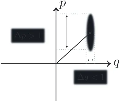
Squeezed states are another member of the family of the minimum uncertainty states. The uncertainty of one quadrature in these states is squeezed at the cost of the in-crease of the uncertainty at the other quadrature. This effect is shown in figure 2.2 using phasor diagram [38].

X

P

§2.4 Quantum States of Light 13

These states can be generated by applying the unitary squeezing operator [38]:

S(ε) =exp(1/2ε∗a2−1/2εa†2) (2.32) Whereε=re2iφ. The level of attenuation and amplification is given by the parameter r = |ε|, which is called the squeezing factor. To produce the squeezed state |α,εi, at first the vacuum state should be squeezed and then displaced [38]:

|α,εi=D(α)S(ε)|0i (2.33)

Further details on squeezed states can be found in references like [38, 39, 31].

2.4.5 Thermal States

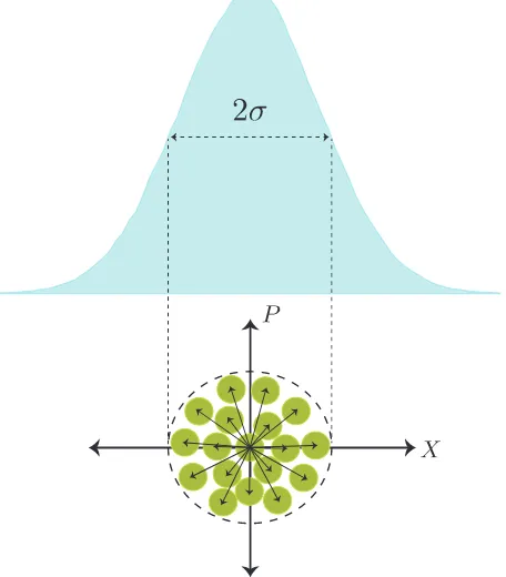
Before proceeding I will briefly mention the classification of the light based on "the standard deviation of their photon number distribution" [31]. This classification is illustrated in table2.1, where ¯n implies the mean value of the photon numbers [31]. As suggested by table 2.1, a perfect coherent light source provides a Poissonian

dis-Table 2.1: Classification of light based on the photon statistics [31] .

Photon statistics Classical equivalent ∆n Super-Poissonian Thermal or chaotic light >√n¯

Poissonian Coherent light √n¯ Sub-Poissonian non-classical <√n¯

tribution, while a sub-Poissonian distribution corresponds to the non-classical light. A super-Poissonian distribution of light appears when there are classical fluctuations in the intensity of light. This form of light is obviously noisier than the coherent light in terms of the classical intensity and quantum photon number fluctuations [31].

Thermal light, which is an electromagnetic radiation emitted from an object due to its temperature has super-Poissonian distribution. Its probability function for a single radiation mode consisting ofnphotons is defined as follows [31]:

Pω(n) =

1 ¯ n+1(

¯ n ¯ n+1)

n _(2.34)

Where ω, n and ¯n refer to the angular frequency of the single radiation mode, the photon number and the mean value of the photon number respectively. This distri-bution, which is famous as"Bose-Einstein distribution", has a variance of [31]:

in equation (2.35) arises from the quantum nature of light, while the second term emerges from the thermal fluctuations, hence has classical origin [31]. More details can be found in ref [31].

2

.

5

Wigner Function

The Wigner function which was initiated by Wigner in 1932, aims to define a prob-ability distribution in quantum mechanics. However, due to the restriction imposed by Heisenberg uncertainty relation [4] on the observation of conjugate variables, this is not in general possible. Hence, the probability distributions in quantum mechan-ics are called "Quasiprobability distributions" [39]. Since in quantum mechanics, the objective is to find the expectation values of the physical observables, it is possible to define a Wigner function in a way that can produce these expectation values. In fact, the correct Weyl inverse transform is also necessary to complete this picture, otherwise the Wigner function is more or less a tool to envisage the quantum states [40]. The inverse Weyl transform ˜Ais defined as follows [40]:

˜

A(x,p) = Z

e−ipy/¯hhx+y/2|Aˆ|x−y/2idy, (2.36) The main characteristic of the inverse Weyl transform is to feature the trace of the product of two operators as follows [40] :

Tr[AˆB] =ˆ 1 h

Z Z ˜

A(x,p)B(x,˜ p)dxdp. (2.37)

Hence, the expectation value of an observable Acan be illustrated as [40]:

hAi=Tr[ρˆA] =ˆ 1 h

Z ˜

ρA dxdp.˜ (2.38)

Where ˆρis the density operator of a pure state|ψibeing defined as ˆρ=|ψihψ|. This leads to designate the Wigner function as [40] :

W(x,p) =ρ˜/h= 1 h

Z

e−ipy/¯hψ(x+y/2)ψ∗(x−y/2)dy. (2.39) Obviously, the expectation value of an observable Anow can be written by employ-ing the Wigner function as [40]:

hAi=

Z Z

W(x,p)A(x,˜ p)dxdp. (2.40)

The projection of the Wigner function onto the x axis provides the probability dis-tribution along the x axis as R W(x,p)dp = ψ∗(x)ψ(x), and its projection on the p axis gives the probability distribution on this axis as R

§2.6 Gaussian States 15

[39].

2

.

6

Gaussian States

A Gaussian state is outlined as any state whose quasiprobabilty distribution, for example its Winger function is Gaussian on the quantum phase space. A general multi-variate Gaussian function has the following form [32]:

f(x) =Cexp(−1

2x

T_Ax+bT_{x), (2.41)}

herex= (x1,x2, ...,xN)T,b= (b1,b2, ...,bN)TandAis an N×Npositive-definite

ma-trix.

In spite of the fact that an infinite-dimensional Hilbert space is associated with continuous-variable quantum states, Gaussian states can be completely characterized through theirfirstandsecondcanonical moments, which are the mean and covariance matrix of their quadratures. Using the compact form of quadrature operators defined in relation 2.16, the first moment is designated as [32]:

da = hRˆaiρ, (2.42)

and the second moment or the so-called covariance matrix is defined as :

σ_ab = 1

2hRˆaRˆb + RˆbRˆaiρ − hRˆaiρhRˆbiρ. (2.43) wherehOˆi_ρ ≡tr[ρO]ˆ is the mean of the operator ˆOevaluated on the stateρ.

The covariance matrix is a real, symmetric, positive definite matrix. From the point of view of statistical mechanics, its elements are the two-point truncated correlation functions between the 2Ncanonical continuous variables [32].

For a bipartite Gaussian state, the covariance matrix can be written as follows:

σ(qˆa, ˆqb, ˆpa, ˆpb) =           

σaaqq σ_abqq σaaqp σ_abqp

σ_baqq σ_bbqq σ_baqp σ_bbqp

σaapq σ_abpq σaapp σ_abpp

σ_bapq σ_bbpq σ_bapp σ_bbpp

           (2.44)

requiresσ_abpq =σ_baqp.

The Wigner function of a Gaussian state has in general a Gaussian form as [32]:

W(X) = 1 πN

1

p

det(σ)

e(X−d)Tσ−1(X−d)_{, (2.45)}

whereX∈R2N_.

According to what mentioned, the covariance matrix contains all the locally-invariant information on a Gaussian state. Hence it is natural to expect that any genuine covariance matrix has to obey certain constraints in order to reflect the re-quirements that the associated density matrix is physical. These rere-quirements are positivity of the covariance matrix in addition to the canonical commutation rela-tions which is described as follows [32]:

σ+iΩ≥ 0 (2.46)

This relation is in fact the strong form of uncertainty principle on the canonical operators, and it is the necessary and sufficient condition that the covariance matrix σhas to meet in order to describe a physical density matrix [32].

2.6.1 Symplectic Transformations and the Gaussian Unitaries

Gaussian quantum information is build based on the symplectic transformations. The symplectic matrices are defined by the following condition [32]:

SΩST= Ω (2.47)

where Ω is the symplectic form described via 2.18. Symplectic matrices are always square(2N×2N), invertible matrices with determinant det(S) = +1 [32].

A very interesting feature of Gaussian states, is the way unitary transformations act on them. A unitary transformation is mapped to realsymplectic transformationson the first and second moments as follows[32]:

ρ0 = UˆρUˆ†−→ d0 = Sd (2.48)

σ0 =SσST (2.49)

hereSis thesymplectic matrixcorresponding to the action of the unitary operator on the Gaussian state. However, this transformation only holds for the unitary transfor-mations whose are at most quadratic in the mode operators {aˆk, ˆa†k}. Because these

unitary transformations preserve the Gaussian nature of the states [32].

2.6.2 Williamson Theorem and Symplectic Spectrum

§2.7 Quantum Measurements 17

described by a covariance matrix σ. This physically corresponds to a normal mode decomposition.The theorem is formalised as follows [32]:

THEOREM: Assume σbe a 2N×2Npositive-definite matrix. Then there exists a symplectic matrix S that diagonalisesσsuch that [32]:

σ= S

N

O

k=1

νk 0

0 νk

ST (2.50)

The N eigenvalues νk collected into ν = diag(ν1, ...,νN), is called the symplectic

spectrum of σ. For a state to be physical, the symplectic eigenvalues must obey ν_k ≥1∀k=1, ...,N. This is equivalent to the condition 2.46 [32].

2.6.3 Standard form of two-Mode Gaussian states

In section 2.6, I mentioned that the vector of first moments can be ruled out by the use of local-unitary operations. For a two-mode Gaussian state, this suggests that the covariance matrix can be described by only 10 elements. For the general case, 2N(2N+1)/2 real parameters are needed to build the covariance matrix (CM). The number of the necessary parameters can further be reduced by applying local unitaries. This will bring the CM to the so-called standard forms. Here, I only limit myself to the two-mode Gaussian states, where by employing a local symplectic operations Sl = S1⊕S2, a covariance matrix σ can be brought to its standard form σ_{s f} [33] :

ST_lσSl = σs f ≡

A C CT _B

(2.51)

where A = diag(a,a), B = diag(b,b), C = diag(c1,c2). The quantities Detσ = (ab−c2₁)(ab−c2₂), DetA=a2, DetB= b2, DetC =c1c2are the four local symplectic

invariants. Hence, the standard form of any CM is unique [33].

Using the standard form of the CM, the symplectic eigenvalues of a two-mode Gaus-sian state can be written as follows [35]:

ν±2 = 1 2[∆ ±

p

∆2_−4I

4] (2.52)

hereI1=DetA, I2 =DetB,I3=DetC, I4=Detσ and∆= I1+I2+2I3.

2

.

7

Quantum Measurements

Due to the usage of "Quantum Measurement", especially "POVM" measurement which implies the Positive Operator-Valued Measure in this thesis, I briefly discuss these concepts here. In quantum mechanics, the measurements are represented by a set of measurement operators like{Mm}, which perform on the state space of the

Considering that |ψi describes the state of the quantum system before the observa-tion, the probability of obtaining the result mfrom the measurement is represented as follows [41]:

p(m) =hψ|M†_mMm|ψi (2.53) With the post-measurement quantum state of the system|ψ0i, given by [41]:

|ψ0i= p Mm|ψi

hψ|M†_mMm|ψi

(2.54)

Besides, the measurement operators should meet thecompletenesscriterion as [41]:

∑

m

M†_mMm = I (2.55)

This guarantees the sum of all the probabilities to be equal to one [41]:

∑

m

p(m) =

∑

m

hψ|M†_mMm|ψi=1. (2.56)

2.7.1 Positive-Operator-Value-Measurement (POVM)

POVM measurement, which implies the "Positive Operator-Valued Measure", is a special case of the general formalism of quantum measurement. The purpose of defining it separately is to provide a straightforward tool to inspect the measure-ment statistics, without looking at the quantum state after the observation. This is applicable for the experiments where the system needs to be observed only once. Again we can assume that the measurement operators Mm function on the

quan-tum system being in the state|ψi, with the outcome probability defined as p(m) =

hψ|M†_mMm|ψi. We designate the operatorEm as [41]:

Em ≡ M†mMm. (2.57)

Considering what mentioned earlierEmis a positive operator, in a way that∑m Em =

I and p(m) = _∑mhψ|M†_mMm|ψi. The complete set of operator {Em} which are

enough to describe the probability distribution obtained from the different measure-ment outcomes is named as a "POVM". (See ref [41] for more details.)

2

.

8

Measurement in Quantum Optics

§2.8 Measurement in Quantum Optics 19

2.8.1 Quadrature Measurement

The homodyne detection technique for quadrature measurement is described in many quantum optics books and texts including ref [39]. Here I briefly review it. The schematic diagram of a balanced homodyne detection is shown in figure 2.3. As it is illustrated the signal beam is interfered with an intense coherent beam called lo-cal oscillator(LO). The local oscillator supplies the phase reference for the quadrature measurement. It should be much more powerful than the signal beam in order to be treated classically. The interested quantity is the subtraction of the two

photocur-LO

Signal

PD

PD

BS

Figure 2.3: Schematic diagram of a balanced homodyne detection. Here LO is the local oscillator, BS is beam-splitter and PD is photo-detector. ˆa_in shows the input mode,αLOis the amplitude of the local oscillator, ˆa0out,1and ˆa0out,2refer to the emerging

output modes of the beam-splitter interfering the signal and local oscillator

rents I1 and I2. These photocurrents are assumed to be proportional to the photon

numbers of the quantum mode reaching each detector defined as follows:

ˆ

n1 =aˆ0out1† aˆ0out1 and nˆ2= aˆ0out2† aˆ0out2. (2.58)

Here ˆa0_out1and ˆa0_out2are the output modes of the beam-splitter mixing the input signal and local oscillator. They are defined as [39]:

ˆ

a0_out1 = √1

2(aˆin−αLO), (2.59) ˆ

a0_out2 = √1

2(aˆin+αLO). (2.60) Hence, the subtracted photon numbers can be written as [39]:

ˆ

Considering the equation (2.11), this can be reduced to [39]:

ˆ n21 =

√

2|αLO|q.ˆ (2.62)

Since the local oscillator carries the phase information, equation (2.62), hence the balanced homodyne detector indeed measures the quadrature component.

2.8.2 Simultaneous Measurement of Two Quadratures

As we know quantum mechanics imposes restriction on the observation of the canon-ically conjugate quantities simultaneously and precisely. However, it is still possible to perform such measurement if we sacrifice the accuracy and allow some extra quantum noise to be involved. Consider we have two conjugate operators ˆq and ˆp, following the commutation relation:

[q, ˆˆ p] =i¯h, (2.63) The concurrent observation of ˆq and ˆp is possible through the definition of other observables described by the relation [39] :

ˆ

Q1 =qˆ+A,ˆ Pˆ2 = pˆ+B.ˆ (2.64)

The operators ˆA and ˆB recount the extra quantum fluctuations introduced to the system in order to perform the simultaneous measurement. They require not to carry any preexisting amplitude [39]:

hAˆi= h_Bˆi=0. (2.65)

And we demand that [39]:

[Qˆ1, ˆP2] =0. (2.66)

In order to fulfill this idea in the quantum optics experiments, the signal beam is divided into two, using a beamsplitter. Each part is then sent to a homodyne mea-surement station, one for observing ˆqand the other for observing ˆp. The key point is to ensure that the local oscillator signals sent to two homodyne detection should have π/2 phase shift. This is generally realized by dividing the same local oscillator into two, by employing a beamsplitter and then applying a phase shift on one arm via a λ/4 wave-plate [39]. This technique is calleddual-homodyne orheterodynedetection. A schematic diagram of the heterodyne (dual-homodyne) measurement is depicted in figure 2.4.

2

.

9

Phase and Amplitude Modulation

§2.9 Phase and Amplitude Modulation 21

LO

LO

Signal

Vacuum

Figure 2.4: Schematic diagram of heterodyne (dual-homodyne) detection. The ele-ments are the same as defined in figure 2.3

2.9.1 Phase Modulation

If we assume to be in a frame rotating at the carrier frequencyΩ, a phase modulated optical field can be written as :

aPM(t) =a0exp(iΩt)exp[iξCos(ωMt)] (2.67)

Where a0exp(iΩt) is the optical field prior to modulation, ωM is the frequency

of modulation, ξ is called "modulation’s depth". ξ = 1 corresponds to complete modulation andξ =0 to zero modulation.

For small modulation depth (ξ ≤ 1), the field aPM(t) can be decomposed into a

component at the laser carrier frequency Ω and sidebands at ωM and −ωM away

from the carrier:

aPM(t)≈a0exp(iΩt)(1+iξCos(ωMt))

=a0exp(iΩt) +i

ξ

2[exp(i(Ω+ωM)t) +exp(i(Ω−ωM)t)]

This shows that the phase modulation transfers optical power from the carrier into sidebands at frequencies ±ωM. These side bands only appear while the phase is

measured. Obviously the intensity will not be modulated as |aPM(t)|2 = a2₀. The

2.9.2 Amplitude Modulation

A beam of light which is amplitude modulated can be expressed as:

aAM(t) =a0exp(iΩt) (1−

ξ

2(1−Cos(ωMt))) (2.68) which can be written as:

aAM(t) =a0exp(iΩt)(1−

ξ 2) +a0

ξ

4[exp[i(Ω+ωM)t] +exp[i(Ω−ωM)t]] (2.69)

We see that the effect of amplitude modulation is to create new frequency compo-nents at±ωM, which are known as the upper and lower sidebands. For completely

modulated light with ξ = 1, the sidebands have exactly half the amplitude of the fundamental component. The resultant intensity is modulated and given by :

I(t) =|aAM(t)|2= I0(1−

ξ

2(1−Cos(ωMt)))

2 _(2.70)

Where I0= a20. More information on phase and amplitude modulation can be found

in ref [34].

2

.

10

Information Theory and Entropy

In this section I briefly review the basic concepts of the classical and quantum infor-mation theory which are based on the definition of entropy.

2.10.1 Shannon Entropy

Shannon entropyis the key concept of classical information theory. For a classical vari-able X with values x occurring with probability px, the Shannon entropy measures

how much information one gains after learning the value of X. There is another complementary view of entropy as a measure of one’s uncertainty before learning the value ofX [41].

The entropy of a random variable is characterized as a function of the probabilities of the different possible values that the random variable can take. The Shannon entropy related to these probabilities is defined as [41]:

H(X)≡ H(p1, ...,pn)≡ −

∑

pxlogpx. (2.71)

§2.10 Information Theory and Entropy 23

2.10.2 Relative Entropy

The relative entropy is a measure of closeness of two probability distributions, p(x) andq(x), on the same index set,x. It is defined as [41] :

H(p(x)||q(x))≡

∑

x

p(x)log p(x)

q(x) ≡ −H(X)−

∑

2.10.3 Shannon Entropy of Continuous Random Variable

Shannon’s entropy can be extended to continuous random variables. AssumeXbe a continuous random variable with the probability density function defined byp(x)on I, where I = (−∞,∞). Then the Shannon’s entropy for continuous random variables is given by [42] :

H(X) =−

Z

I p(x)logp(x)dx, (2.73)

Although it has many properties of Shannon’s entropy of discrete variables, un-like that it can become infinitely large or negative. In addition, the Shannon’s entropy for continuous random variables does not necessary remain invariant under a change of variable, while Shannon’s entropy of discrete variables remains invariant [42].

2.10.4 Joint Entropy

The joint entropy quantifies one’s total uncertainty about the pair of random variables (X,Y). It is naturally defined as [41]:

H(X,Y)≡ −

∑

x,y

p(x,y)logp(x,y). (2.74)

2.10.5 Conditional Entropy

If we have a pair of random variables (X,Y), by performing a measurement on the random variableYwe can learn its value and acquireH(Y)bits of information about the pair. The conditional entropy quantifies our lack of knowledge about the pair (X,Y), on average, given the fact that we know the value of Y. It is simply defined as [41]:

H(X|Y)≡ H(X,Y)−H(Y). (2.75) Another way to express It, is the lack of knowledge ofXwhen the state ofYis in the ythstate, weighted by the probability forythoutcome as [44] :

H(X|Y) =−

∑

y

whereyis the outcome of the measurement performed on subsystemY. Conditional entropy can be shown schematically using the ’entropy Venn diagram’ depicted in figure 2.5.

H(X)

H(Y)

H(X:Y)

H(X|Y)

H(Y|X)

Figure 2.5: Entropy Venn diagram, showing the relationship between different en-tropies [41].

2.10.6 Mutual Information

The mutual information quantifies how much information two random variables (X,Y)have in common [41]. It is defined as [30]:

H(X :Y) =H(X)−H(X|Y) (2.77) This can be seen in ’entropy Venn diagram’depicted in figure 2.5. The mutual infor-mation quantifies the average decrease of entropy ofXwhen the value ofYis known [30]. Using the ’Bayes’ rule, which defines the conditional probability for classical variables as p_x|y= pxy/py [43], equation (2.77) can be written equivalently as [30]:

H(X:Y)≡ H(X) +H(Y)−H(X,Y). (2.78) Further information can be found in ref [30, 41, 43]

2.10.7 von Neumann Entropy

In classical information theory we calculate the uncertainty of the classical probability distribution using Shannon entropy. Quantum state can be described similarly with density operatorsρ, and Shannon entropy can be generalized for quantum states to Von Neumann entropy [41].

§2.10 Information Theory and Entropy 25

S(ρ) =−Tr(ρlogρ) =H(λ) (2.79) Whereλ= λi are the eignevalues of the state. Here also the logarithms are taken to

base two and 0 log 0≡0.

2.10.8 Quantum Mutual Information and Conditional Entropy

Classical mutual information described by equation (2.78) can be easily generalized to quantum mutual information by simply replacing the Shannon entropy by Von Neumann entropy and the classical probability distributions by density matricesρas follows [30]:

I(ρXY) =S(ρX) +S(ρY)−S(ρXY) (2.80)

However, equation (2.77) cannot be easily generalized to quantum states, as to define the conditional entropy H(X|Y) one needs to define the state of X given the result of the measurement performed on the state ofY. This is more obvious by looking at the measurement-based version of conditional entropy defined by the relation 2.76. Such statement is ambiguous in quantum mechanics until the set of the measure-ment which will be performed on the stateY is selected [30]. In order to define the quantum analogue of the measurement-based conditional entropy a set of (POVM) with elements{Ey= M†yMy}is assumed to perform on subsystemYwithyto be the

outcome of the measurement (see subsection 2.7.1 for description on POVM). The probability of obtaining the outcome y is py = tr(ρxyEy) and subsystem Xis left in

the conditional state of ρ_X|y = trY(ρXYEy)/py. This allows us to write the quantum

version of measurement- based conditional entropy as S_{Ey}(X|Y) ≡ _∑y pyS(ρ_X|y). Hence, the quantum analogue of mutual information defined by equation (2.77) can be written as [43]:

max_{Ey}J(X|Y)≡S(X)−S_{Ey}(X|Y) (2.81) The quantity max{Ey}J(X|Y)which is maximized over all possible POVMs is called

one way classical correlations [29].

2.10.9 Holevo Bound

defined as follows [41] :

H(X:Y)≤S(ρ)−

∑

x

pxS(ρx), (2.82)

Whereρ =∑_xpxρx. This refers to the situation when Alice prepares a stateρX, while

X =0, ...,nwith probability of occurring asp0, ...,pn, and Bob operates a POVM

mea-surement on the state with elements{Ey}={E0, ...,Em}, andybeing the outcome of

the measurement [41]. (See ref [41] for more details).

2

.

11

Quantum Correlations

Since the focus of this thesis is on Quantum Correlations, I specify this section to describe the well-known forms of quantum correlations and the way to quantify them especially in Gaussian states.

2.11.1 Entanglement and non-locality

When two physical systems have an interaction with each other, some form of cor-relation with a quantum nature is created between them, which remains even when the two systems get specially separated. This suggests that, if one performs a mea-surement on a local observable on the first system, the state of the second system, no matter where it is, is modified instantaneously. This phenomenon, named by Ein-stein, Podolsky and Rosen as "spooky action at a distance" [3], is calledentanglement which is the non-classical and non-local quantum correlation. However, non-locality and entanglement are a bit different. It can be understood from the general frame-work of no-signalling theories which demonstrate more non-local features than the quantum mechanics [33, 36]. According to Bell [33, 37], non-locality is a channel in nature which allows one to distribute correlations between distant parties, in a way that the correlations are not pre-determined at the source, and the correlated random variables can be generated when distant parties perform local measurements on their subsystems. Quantum mechanics describes this channel as an entangled pair [33]. As I will describe in the following chapters this characteristic of nature is harnessed in secure quantum communications.

Considering the importance of quantum entanglement, it is desirable to have an op-erational criterion to examine if a given state is entangled or not. As I will show shortly, forpure statesof the composite quantum system, it is relatively easy to quan-tify entanglement. However, the situation is more complicated withmixed states, as a mixture can be in many different ways where no one can extract all the information it contains [33].

2.11.2 Entanglement Criteria for Pure Bipartite States

A pure quantum state |ψi ∈ H = H1⊗H2 is entangled if it cannot be written as a

§2.11 Quantum Correlations 27

|ψi= |φi1⊗ |χi2 ≡ |φ,χi. (2.83)

where|φi1 ∈H1and|χi2∈ H2.

In order to quantify entanglement one can write a pure quantum state in its unique Schmidt decomposition [41] as follows [33] :

|ψi=

d

∑

k=1

λk|uk,vki, (2.84)

where

d=min{d1,d2} , (2.85)

λk ≥0, d

∑

k=1

λ2_k =1. (2.86)

The local bases {|uki} ∈ H1 and {|vki} ∈ H2 are the Schmidt bases, the positive

numbers {λk}are the Schmidt coefficients and the number d of the non-zero terms

in the Schmidt number. It can be seen that the product states |ψi = |φ,χi can be automatically written in the Schmidt form whend= 1. In other words if a state can be written as Schmidt decomposition with only one coefficient, then it is necessarily a product state. Hence, a pure state|ψiof a bipartite system is entangled if and only ifd>1 [33].

2.11.3 Entanglement Criteria for Mixed States

A mixed state can be written as a convex combination of pure states :

ρ=

∑

k

pk|ψkihψk| (2.87)

Now the problem is that this decomposition is not unique, unless ρ is already a pure state. This means that the mixed states can be prepared in many different ways which makes the entanglement’s quantification very difficult. Considering the ambiguity on the state preparation, no one knowsa prioriif the correlations between the subsystems arose from a quantum interaction or were induced by means of LOCC (Local Operations and Classical Communications) which causes classical correlations [33].

A mixed quantum state of a bipartite system, described on the Hilbert space H=H1⊗H2, is separable if and only if it can be written as follows :

ρ=

∑

k

pk(σk⊗τk). (2.88)

en-tangled . However, this is a very impractical way of checking if a state is enen-tangled or not. Since deciding entanglement or separability according to this definition would require one checks all the infinitely many decomposition of a state ρand look for at least one of them to be in the form of 2.88. Hence, several operationalcriteria have been developed to check entanglement in mixed quantum states [33]. In addition, developing a criterion for checking the inseparability will be dramatically simplified if we restrict ourselves to the certain class of quantum states. Considering that the focus of this thesis is on the continuous-variables and particularly on Gaussian states, here I only present two entanglement criteria applicable to the two-mode Gaussian states. The first one is theDuan inseparability criterionintroduced by Duanet al. [47], which provides a necessary and sufficient condition for the inseparability of two-mode Gaussian states. The second one is the EPR-paradox criterion introduced by Reid [46] which quantifies the degree of EPR paradox of a state.

2.11.4 Duan Inseparability Criterion

The Duan inseparability criterion quantifies the strength of entanglement of a quan-tum state. For the case of two-mode quadrature entangled state, It is defined as [48]:

I =

q

∆2_xˆ

a±b∆2pˆa±b (2.89)

where∆2_Oˆ

a±b=minh(δOˆa±δOˆb)2i/2 . IfI <1, the state is inseparable. I =0

cor-responds to the best possible entanglement obtained from combining two perfectly squeezed beams [48].

2.11.5 EPR Paradox Criterion

EPR criterion measures the degree of the EPR paradox, introduced by Einstein, Podolsky and Rosen in 1935 [3]. It is based on the ability of a state to produce an apparent violation of the Heisenberg uncertainty relation between two conjugate variables. A quantifying measure of an EPR violation for the continuous variables was introduced by Reid in 1988 [45, 46]. This criterion which is more restrictive than the Duan inseparability criterion, is defined as the product of the conditional variances of the phase and amplitude quadratures as follows:

eab =∆qˆa|b∆pˆa|b <1 (2.90)

e_ba =∆qˆ_b|a∆pˆ_b|a <1 (2.91) The conditional variances are defined as :

∆qˆ_a|b =∆qˆa−

|σ_abqq|

∆qˆb

§2.12 Summary 29

whereσ_abqq is the covariance and∆qˆa and∆qˆbare the variances (please see 2.44).

Sim-ilar relation applies for other quadrature ˆp or the other direction of the conditional variances. The conditional variance quantifies the reduced uncertainty on subsystem afollowing a measurement on subsystemb. This gives a measure where the subsys-temsa andbare not perfectly correlated, but by performing a measurement on one subsystem some information can be gained about the other subsystem.

A state demonstrates an EPR paradox if the product of the conditional variances of the two orthogonal quadratures is below one. Satisfying this criterion is a sufficient but not the necessary condition for a state to be entangled.

2.11.6 Quantum Discord

While it was thought previously that the absence of entanglement implies the classi-cality of the states, recent research has shown that some form of quantum correlations can exist even in the separable states. This notion of quantumness which was first discovered by Ollivier and Zurek [30] is calledquantum discord. This is an important form of quantum correlations that attract lots of attentions during recent years. This concept will be elaborated in the next chapter.

2

.

12

Summary