Indium Recovery in an Electrochemical Flow Reactor. Simulation and Experiment

Int. J. Electrochem. Sci., 12 (2017) 3516 – 3536, doi: 10.20964/2017.04.24

International Journal of

ELECTROCHEMICAL

SCIENCE

Indium Recovery in an Electrochemical Flow Reactor.

Simulation and Experiment

Yung-Fu Wu* and Yu-Sheng Wang

Department of Chemical Engineering, Ming Chi University of Technology, 84 Gungjuan Rd. Taishan, Taipei 24301, Taiwan

*

E-mail: [email protected]

Received: 10 January 2017 / Accepted: 17 February 2017 / Published: 12 March 2017

This study investigated the numerical simulation and experiment of a continuous indium removal process from wastewater by using an electrochemical flow reactor. The competition between hydrogen evolution and indium reduction was taken into consideration. The simulated residual indium distribution accompanying with flow field corresponds to the removal performance of experiments. The concentration field indicates a two-stage development between the electrodes. In the second stage, an apparent removal of indium takes place, but a steady state reached after a long-term incubation at a low flow rate. However, the removal ratio rises quickly and levels off after a short-term incubation at a high flow rate. At 762 mL/min, 90% or more of indium in wastewater can be removed, but only 50% or less of indium can be reduced at 7620 mL/min. The flow cell takes a compromise between throughput and efficiency if an optimal operation is adopted. The optimization on the basis of energy consumption and equipment cost shows that two flow cells in series operated at 3810 mL/min may be more economical than a unit cell at any flow rate in the influence of hydrogen evolution.

Keywords: Numerical simulation; Electrochemical Flow Reactor; Indium; Wastewater.

1. INTRODUCTION

application is getting involved in the field of solar cells, electrochromic devices and biochips [4-6]. Consequently, reducing the use of indium currently has few chances of success but recovering from a large amount of indium waste might be feasible. If not recovered, the waste may cause adverse impacts to the environment and public health. It is known that indium and its compounds might damage the heart, kidney, liver, joint or bone [7-9]. Therefore, indium removal from waste and then reuse in manufacture should be a best way for sustainable use and environmental protection.

The indium waste mainly comes from fabrication and disposal of optoelectronics including ITO films. The primary method of depositing ITO films on substrates is by sputtering. However, roughly 70% of indium leaves on the used target or falls on the sputtering chamber when the used target is replaced. Accordingly, the used target and chamber residue are the first type of indium recovery source. Deposited ITO film is patterned using lithographic methods during mass production, so the second recovery source of indium comes from the etching wastewater. Although the wastewater generally contains indium less than 2 wt%, the residual indium can be recovered straightforward using wet-type techniques. This type of wet techniques can be implemented in-line, but the solid waste only can be treated off-line. In addition, the third type of the recycling indium source can be found in discarded displays [10]. Although the procedure is more complicated than the treatment of used targets, the available amount of indium from an annual LCD disposal is considerable.

The first step to obtain indium powders from waste is mainly by scraping and grinding [11-13]. The powders experience size classification to enrich indium, followed by dissolving in aqueous solution for subsequent refining. The solution process includes extracting indium by solvents [14-17], leaching the scraps in strong acid [18-20], and adding alkaline to form indium precipitate [21-23]. Afterward the indium-contained solution experiences electrorefining to form highly pure indium. For the 2nd type of waste, recovering indium from etching solution is straightforward a wet process. During the ITO etching, a widely-used etchant includes HCl for breaking In–O bond [24]. The corresponding etch wastewater thus contains indium ions and follows an electrochemical path to produce pure indium.

Even though several methods of indium recovery operated at high temperature have been suggested [23, 25], the electrorefining is usually the last procedure to obtain highly pure indium metal from waste [26]. It is well know that a rotating electrode system is an important tool for electrolysis, electroplating or electrochemical analysis. In comparison with a stationary electrode, the rotation of an electrode induces fluid flow and convective mass transport. Several designs for rotating electrodes have been investigated, but the rotating cylinder system attracts much interest in electrochemical industry [27]. A rotating inner cylindrical electrode accompanying with a stationary concentric outer electrode is the most often adopted design. Although the governing equations of the transport phenomena and reactions can be used to describe an electrochemical system well, the closed form or exact solutions were rarely obtained. Conventionally, the mass transport in a practical electrochemical reactor was predicted via empirical analysis with dimensionless Sherwood (Sh), Reynolds (Re) and Schmidt (Sc) numbers. The definitions of these numbers are described as follows:

Sh k dm

D

Re rdu

m

= (2)

Sc d m r

= (3)

In which, D is diffusivity, d is characteristic length, u is fluid velocity, r is fluid density, m is fluid viscosity and k_m is mass transfer coefficient. Since k_m is linearly proportional to limiting current, the electrochemical reaction term can be involved in this dimension analysis. The correlation of Sh, Re and Sc corresponding to a specified system can be then obtained by experiments. The empirical correlations of a rotating cylinder system have been developed by Lévêque since 1928 [28]. Various types of modified correlations based on detail system geometry and operation parameters were then suggested [29]. Meanwhile, the work by direct numerical simulation of transport equations was also in progress to provide the message of potential, current and concentration distributions in an electrochemical reactor, so-called tertiary current distribution [30-33]. Prediction of time-dependent electrolysis and applicability of specified boundary conditions are regarded as the primary advantage of direct numerical simulation. Especially when the electrochemical process must involve the bulk materials change with time and the fluid flow profile with space, direct numerical simulation can assist the process design. However, little research has devoted on the continuous electrolytic process of metal recovery at transient state via direct numerical simulation of tertiary current distribution. Indium removal from wastewater was seldom investigated using a flow type of the electrochemical reactor. The issue of optimal operation based on energy consumption was rarely examined in past work of direct numerical simulation.

Therefore, this study investigated the numerical simulation of a continuous indium removal process using an electrochemical flow reactor. The tertiary current distribution accompanying with flow field can be obtained, and the effects of the geometry, operation parameters and side reactions in this system were explored. Especially the competition between hydrogen evolution and indium reduction was taken into consideration. The corresponding experiments of a flow process were then performed to compare with the transient simulation. Finally this study elaborated the optimal operation on the basis of energy consumption and cost.

2. EXPERIMENTAL METHODS

The electrolyte containing 100 ppm indium was prepared using InCl3 and 0.1 M HCl. Before

the electrolysis, the prepared electrolyte flowed through the annular space and overflowed from the top peripheral edge of the cell continuously for 5 min at 298 K. Meanwhile, the rotating cathode initiated from the stationary state to the steady state at the required angular velocity. Afterward, a constant cell voltage was applied across the anode and cathode using a potentiostat (PGSTAT30, Metrohm Autolab B.V.). During the operation, the treated solution was sampled at the overflow position to detect the variation of residual indium content. The sampled time was selected in 3 hours to investigate the time dependence of removal ratio. After each sampling, the residual indium content was analyzed using inductively coupled plasma optical emission spectrometry (ICP-OES, Perkin Elmer 3100XL).

50 mm

Shaft

12 mm

Cathode Anode

1.50 V Potentiostat

100 rpm

Modulated Speed Rotator

Overflow

52 mm

150 mm

Inflow

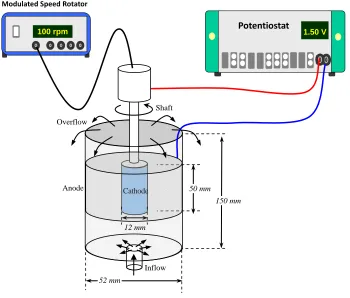
Figure 1. Schematic diagram of flow cell for indium recovery. The electrolyte enters from the bottom of the cell and overflow out of the cell. The cathode rotates at 100 rpm but the anode is fixed. The setup is close to an axisymmetric system.

3. MATHEMATICAL MODEL

during electrorefining, i.e. a steady-state flow field can be assumed in this study. When a low rotation speed is selected to operate the metal removal process, a laminar flow through the cell can be expected. Similar assumptions were used in the research of Mandin et al. [30, 31]. Therefore, Navier-Stokes equation in a cylindrical coordinate are employed:

(ru) 0

Ń × = (4)

2

[ ( ) ( ) ]

3

T

p g

u u u u u I

r ×Ń = - Ń + Ń × Ń + Ńm - mŃ × + r (5)

where u is the velocity vector and p is the pressure, ρ and μ are the density and viscosity of the electrolyte, and I is the identity matrix. Even though the bulk indium content decreases with time, the density of the dilute electrolyte is regarded as a constant, meaning that the natural convection was neglected herein. However, the inlet flow and the forced convection from the rotating electrode must influence the materials balance in the electrolyte. The balance equation is expressed as:

( ) 0

i

i i i i i l i

c

D c z Fc c

t m f

¶

+ Ń ×- Ń - Ń + =

¶ u (6)

where c D z m_i, _i, , _{i i} are the concentration, diffusivity, charge number and mobility of ion species i, respectively, and F is Faraday’s constant. This study considers four ions, including H+ ,

OH- , 3

In + and Cl- . All of these ion species are confined to the electroneutrality assumption: 0

i i i

z c =

ĺ

In Eq. (6), f_l represents the electrical potential in the electrolyte and the potential gradient Ńf_l

provides a driving force for ion migration. In addition, the concentration gradient Ń and fluid flow c_i field u produce the other driving forces for ion movement. These driving forces dominate the current density vector i_l in the electrolyte:

( )

l i i i i i i l

i

i =

ĺ

On the electrode surface, the current density is determined by the electrochemical reaction rate. In this study, two cathodic reactions are considered. One is the reduction of indium ions, contributing to the indium removal from wastewater; the other is the evolution of hydrogen, competing with indium reduction.

3

In + +3e- ƒ In (9)

2 2H+ 2e- H

+ ƒ (10)

The reaction rate of indium reduction depends not only on the electrode potential fs but also

on the surface concentration of In3+, denoted as cs. The current density resulted from indium reduction

can be expressed by the concentration dependent Butler-Volmer equation:

(11)

where i_0,1 and a₁ are the exchange current density and transfer coefficient of indium reduction, T is the temperature, R is the universal gas constant, η is the overpotential and c_b is the bulk concentration. The initial c_b is 100 ppm. Furthermore, the overpotential is defined as:

s l Eeq

The hydrogen evolution frequently takes place in the aqueous electrolysis. The current density corresponding to hydrogen evolution can be assumed to depend only on the applied potential due to a small difference between surface and bulk concentrations of H+ in a strong acid:

(12)

where i_0,2 and a₂ are the exchange current density and transfer coefficient of hydrogen reduction. Hydrogen evolution consumes partial of the applied energy, leading to a decreasing current efficiency of the electrolytic process.

r = 0

lE dS

dB

Shaft

Rotating cylinder electrode

Anode

Electrolyte

dE

Exit

Inlet

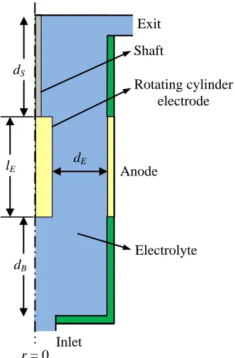
Figure 2. Geometry of the axisymmetric flow cell in which the shaft immersion depth is d_S

(adjustable), the electrode length is l_E (fixed at 50 mm), the distance from electrode to cell bottom is d_B (adjustable), and the distance between anode and cathode is d_E (fixed at 20 mm).

The total current density on the cathode determines one of the boundary condition of the electrolyte:

1 2

i= i +i (13)

On the other hand, the total current density on the anode is related to the oxygen evolution:

2 2

1

H O 2H O 2e

2

+

-+ +

ƒ (14)

Under the assumption of excess H+ in the electrolyte, the current density on the anode is independent of H+ concentration:

(15)

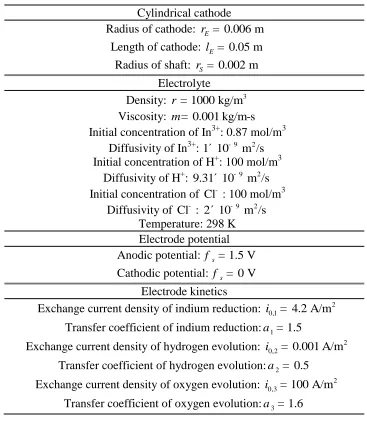
On the container wall of the reactor, instead of the location of the anode, there are no fluxes of mass transport. Near the top cap of the cell, the materials only transport through the perimeter via overflow. To summarize, Table 1 shows all of the parameters and properties required in this simulation [34, 35].

The software COMSOL Multiphysics® 4.4 was used to solve this problem. Figure 2 indicates the domain and boundaries of the electrolyte. The electrolyte domain was divided into 61544 triangular elements with element sizes ranged from 5 10 m´ -4 to 5 10 m´ -6 . The mesh density in the vicinity of the boundaries was higher than that in the bulk region, facilitating the calculation of the high gradient conditions.

Table 1. Parameters used in the numerical simulation.

Cylindrical cathode Radius of cathode: r_E= 0.006 m

Length of cathode: l_E= 0.05 m Radius of shaft: r_S = 0.002 m

Electrolyte Density: r =1000 kg/m3 Viscosity: m= 0.001 kg/m-s Initial concentration of In3+: 0.87 mol/m3

Diffusivity of In3+: 1 10 m /s´ -9 2 Initial concentration of H+: 100 mol/m3

Diffusivity of H+: 9 2 9.31 10 m /s´ Initial concentration of Cl- : 100 mol/m3

Diffusivity of Cl- : 9 2 2 10 m /s´ Temperature: 298 K

Electrode potential Anodic potential: f_s=1.5 V Cathodic potential: f_s = 0 V

Electrode kinetics

Exchange current density of indium reduction: i_0,1= 4.2 A/m2 Transfer coefficient of indium reduction:a₁= 1.5

Exchange current density of hydrogen evolution: i_0,2= 0.001 A/m2 Transfer coefficient of hydrogen evolution:a2 = 0.5

Exchange current density of oxygen evolution: i_0,3=100 A/m2 Transfer coefficient of oxygen evolution:a3= 1.6

4. RESULTS AND DISCUSSION

the anode. Furthermore, the effects of the cell parameters were studied. The corresponding notations for 3D-view and cross-sectional view can be found in Figure 1 and Figure 2, respectively.

(a) (b)

(c) (d)

Figure 3. Streamlines in the flow cell with l_E= 5 cm/d_S = 5 cm/d_B= 5 cm operated at flow rates of (a) 762 mL/min; (b) 3810 mL/min; (c) 7620 mL/min; (d) 38100 mL/min, respectively.

According to the steady state assumption, the velocity and pressure profiles can be solved, and the simulation results of streamlines are shown in Figure 3. From the cross-sectional view, the electrolyte enters the cell from the inlet tube, resulting in a flow expansion and a vortex at the bottom corner. Except for the cell corner, the electrolyte almost flows by the electrodes in a parallel stream mode. Then the electrolyte meets the cap of the cell and thus turns along the radial direction to exit the

lE dS

dB

Inlet

cell. It is noted that the vortex found in the bottom corner of the cell depends on the flow rate and the distance from the cathode to cell bottom (d_B). When the flow rate increases, the vortex-occupied area grows, as can be seen in Fig. 3(a)-(c). It can be anticipated that some metal ions might circulate around this corner, indicating that the cell design should be improved to reduce the retention of electrolyte. On the other hand, when the electrolyte enters the region between the anode and cathode, a slight extent of flow contraction occurs, especially affecting the flow near the rotating cylinder corner. At this corner, the electrolyte loses partial of kinetic energy to turn its flow direction. If d_B is small, as shown in Fig. 4(a), the decrease in the flow velocity is large especially in an operation of high flow rate. Otherwise, the hindrance of flow can be reduced when d_B is increased, as shown in Fig. 4(b), but the vortex at the cell bottom grows to increase the circulation of the electrolyte. These phenomena seem to indicate a trade-off operation in the view of electrolyte flow. On the basis of the simplified model, the effect of the flow pattern on metal removal is investigated as follows.

(a) (b)

Figure 4. Streamlines in flow cells with (a) l_E= 5 cm / d_S = 7.5 cm / d_B= 2.5 cm and (b) 5 cm

E

l = /d_S = 2.5 cm/d_B= 7.5 cm operated at a flow rate of 7620 mL/min.

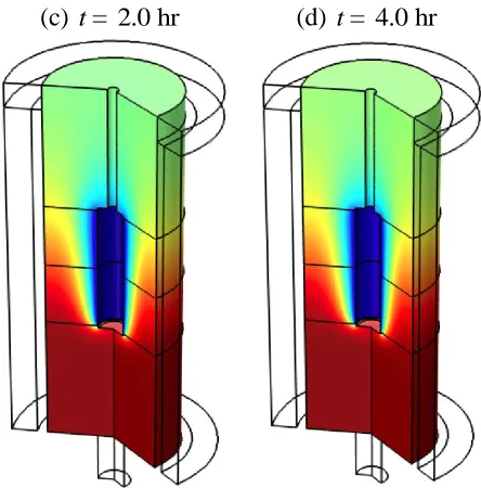
During the steady-flow operation, the indium concentration profile can be obtained from the simulation of tertiary current distribution. Figure 5 exhibits the relative concentration profile of In3+ for a cell with d_B= 5 cm and d_S = 5 cm, while Figure 6 shows those for a cell with d_S = 2.5 cm and

7.5 cm

S

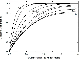
d = . The relative concentration is defined as the ratio of a local concentration to the inlet one. It can be seen that In3+ ions carried by the inflow consume at the cathode, causing a low profile near the cathode surface and meanwhile building up a concentration gradient between two electrodes, as shown in Figure 5(a) from blue zone (low concentration) to red zone (high concentration). Since the concentration gradient can describe the region of diffusion layer, the thickness of the diffusion layer is found to increase with time. At the anode, no consumption of In3+ ions occurs. The surface concentration is, however, reduced with time, meaning the bulk concentration between two electrodes

lE dS

decreased with time. The reduction of concentration also can be found in Figure 7(a), showing the distribution of In3+ concentration along the connection line between the middle points of the cathode and anode. The results indicate that the surface concentration decreases to almost zero in a short period. Then the diffusion layer extends with time under a spiked bulk concentration until a characteristic time t₁. After the characteristic time, the thickness of the diffusion layer approaches the distance between the cathode and anode, accompanying with a gradual decrease in the bulk concentration. In conventional models for metal removal in a batch cell, the local diffusion layer thickness is hardly analyzed by using overall mass transport coefficient [33]. Alternatively, the research employed a Nernst diffusion layer model to assume the layer thickness depends only on the rotation speed of electrode, and then the diffusion layer will be fixed in the vicinity of electrode [32]. However, the results from our model show that the diffusion layer can grow thicker with time until the layer edge attains the counter electrode, which is more practical in bulk electrolysis than those models often used in electroanalysis. Accordingly, the development of In3+ concentration gradient can be divided into two stages via the characteristic time t₁. The simulation results indicate that the characteristic time t₁ changes with the inflow rate. When the flow rate is high, the characteristic time gets long, as shown in Figure 7(b). In the former stage, the consumption of In3+ ions can be seen from the extending diffusion layer, while the removal of In3+ ions is mainly based on the decreasing maximum concentration in the latter stage. It is expected that a small current density and consumption rate of In3+ ions is observed after the characteristic time t1. Furthermore, the concentration profile almost stops changing with time after the second characteristic time t2. The cell can keep stable due to the balance between the consumption of electrolysis and the compensation of inflow. In other words, the steady concentration profile should depend on the flow rate of the cell. As shown in Figure 7, a larger flow rate gives rise to a higher residual concentration at steady state, corresponding to a lower removal performance.

(c) t= 2.0 hr (d) t= 4.0 hr

Figure 5. Relative concentration profiles of In3+ in a flow cell with l_E= 5 cm/d_S = 5 cm/d_B= 5 cm operated at 7620 mL/min.

The removal ratio is estimated from the concentration difference between the inlet and exit, as shown in Figure 8. The removal ratio at the operation of 762 mL/min attains to 90% or more, while the ratio at 7620 mL/min reduces to 50% or less.

0.5 hr

t=

(a)

(c) (e)

Exit

An

o

d

e

C

ath

ode

4.0 hr

t=

(b) (d) (f)

2.5 cm

S

d =

7.5 cm

B

d =

5 cm

S

d = 5 cm

B

d =

7.5 cm

S

d =

2.5 cm

B

d =

Figure 6. Relative concentration profiles and contours of In3+ in flow cells with l_E= 5 cmoperated at 7620 mL/min.

The experimental data with error bars at various flow rates are also plotted in Figure 8(a). Although small discrepancies are found between the experimental average and simulation results, the trend of indium removal still can be described by our model.

(b)

Figure 7. Relative concentration profiles of In3+ along the middle line between two electrodes in a flow cell with l_E= 5 cm/d_S = 5 cm/d_B= 5 cm at (a) 762 mL/min; (b) 7620 mL/min.

When the position of the cathode is altered, Figure 8(b) shows that the simulation overestimates the removal ratios, indicating a larger drag effect on the electrode bottom than expected.

However, the dependence of d_S on the measured removal ratios is still discernible in the incubation period, similar as the trend in our model.

(b)

Figure 8. Removal ratio of In3+ in flow cells operated (a) at various flow rates with d_S = 5 cm; (b) at 7620 mL/min with various d_S. The lines and symbols represent the simulated and experimental data, respectively.

Note that the second characteristic time t2 also can be estimated in Figure 8 by extrapolation of the transient state. The estimation shows that the incubation period is long when the flow rate is low, even though the final removal performance is advantageous at a low flow rate. If the operation period and cost are limited to practical consideration, our simulation points out an optimal flow rate.

The whole removal performance of the flow cell is not only related to the concentration profile at the middle line between the two electrodes, but also dependent on the concentration profile at various corners. Figure 9 shows the mass flux of In3+ ions in the flow cell operated at 762 mL/min with a configuration of lE= 5 cm/dS = 5 cm/dB= 5 cm. The moving direction (white lines) indicates the

(a) (b) (c) (d) SI Unit

Figure 9. Mass flux of In3+ in a flow cell operated at 762 mL/min with 5 cm

E

l = / d_S = 5 cm / d_B= 5 cm at (a) t= 0.02 hr ; (b) t= 0.2 hr ; (c) t=1.0 hr ; (d) 4.0 hr

t= .

The simulation results in Figure 8(b) indicates that the steady removal performance is slightly raised when the depth of the shaft immersed in the electrolyte (d_S) is increased, but the difference between various d_S is indistinguishable, approximate 0.4%. On the other hand, the transient states between the operations with various d_S are discernable. As d_S = 2.5 cm, the removal performance is effective for a short-term operation in comparison with those at d_S > 2.5 cm. For example, at 0.3 hr, the removal ratio of the operation at d_S = 2.5 cm is four times as large as that at d_S = 7.5 cm, indicating that agitation or circulation effect could be reduced if the exit is set close to the cathode. Figure 6 exhibits the similar phenomena. The area with low concentration (green zone) is apparently larger when d_S = 7.5 cm than that when d_S = 2.5 cm. The results with changing d_S show that the mass transport in the top region of the cell is more important than that in the bottom region at the transient state.

As mentioned above in the section of mathematical model, the electrode kinetics and mass transport commonly control the removal rate in this study, but herein the electrochemical removal of indium is regarded as a mass-transport limited only process facilitating to compare with the results from previous research. Then the bulk electrolysis of indium follows a 1st-order rate law [33]. Consider a steady single-pass reactor, where a steady volumetric flow rate (Q) of electrolyte is assumed. The steady concentration at exit (c_out) is then given by

CE out in

I

c c

nFQ



  (16)

where c_in is the concentration at inlet, I is the current passing through electrodes, and _CE is the current efficiency defined by i₁/(i₁i₂) from eqns.(11) and (12). Due to the steady removal ratio (r_R) is defined as

An

o

d

e

C

ath

ode

Inlet

1 out R in c r c

  (17)

The averaged mass transport coefficient (k_m) in a flow cell can be represented as

CE

m R

in

I

k r Q

nFc



   (18)

In a concentric cell, Sherwood number (Sh) is typically estimated from the hydraulic diameter, twice of the distance between two electrodes (2dE). Therefore,

2 2

Sh k dm E d r QE R

D D

  (19)

At flow rate of 762 mL/min, Sh= 381.

However, for a batch rotating-electrode cell, Mizushina’s correlation gives that [36]: 0.50 0.33

Sh= 0.74Ta Sc (20)

where Ta is Taylor number: 1.5 0.5 Ta r wd rE E

m

= (21)

According to Mizushina’s correlation, Sh= 415 at w100 rpm. It is known that Sherwood number (Sh) is proportional to mass transport coefficient (km), but this km shows only a mean property of a whole reactor. Moreover, the value of km depends much on the choice of characteristic length in the reactor. In a typical correlation such as eq.(20) for a batch cell, the length of the electrode, the depth of immersed shaft and the distance between electrode and cell bottom are not included, which could lead to an unrepresentative estimation for mass transport. However, we considered not only the effects of various cell dimensions but also the influences of inlet and exit in this study. These factors must induce an essential difference in hydrodynamics. Our results indicate that the axial flow in a flow cell decreases km and Sh, while the circulation flow in a batch cell increases them. In a practical application, in-line treatment and long-term operation should be taken into consideration. A continuous process via a flow cell might be preferred because the treated wastewater can be reused and the recovered metal may not redissolve with O2 generated at anode [37]. Furthermore, an electrochemical reaction often

leads to a density gradient due to the change of ion concentration in electrolyte, then causing that the mass transport is dominated by natural convection, rather than forced convection [30, 31]. However, mass transport in a flow cell is inevitably determined by forced convection due to the continuous supplement of raw electrolyte. Therefore, Sherwood number in a laminar flow cell is less than that in a batch cell at a common rotating speed of electrode.

If the concentric-cylinder cell is used, the mass transport can be described by the correlation [39]:

1/ 3 1/ 3 2 1/ 3

Sh 1.85Re Sc ( E)

E

d l

= (22)

where l_E is the length parallel to the axial flow. This correlation gives that Sh=120 at flow rate of 762 mL/min. Accordingly, the Sherwood number for an electrochemical flow cell falls between those of batch cell and stationary concentric-cylinder cell. It indicates that the axial flow retards the mass transport from the bulk solution to the electrode surface, while the swirl flow enhances. Consequently, wastewater treatment by a flow cell takes a compromise between large throughput and high efficiency if an optimal operation is adopted.

In view of an optimal operation on a basis of cost, a target removal ratio (rt) is assigned first

and then the minimum cost under rt can be estimated. In some cases, N unit cells in series are required

to reach the target removal ratio (rt). The cost of a system is divided into the operation part and

equipment part. The former depends on the energy consumption, while the latter relates to materials and life time of a cell. The total energy consumption in a unit cell can be expressed as:

3 2 0 0 2 t t T in Q t

E IEdt dt

A

 _

 





The three terms on the right-hand side represent the energy for pumping fluid, the energy for removing metals by an electrochemical reaction and the energy for rotating an electrode, respectively. According to the steady drag force by fluid on a cylindrical surface, the torque (T) of an electrode is averagely estimated as [40]:

2 2

2 2

4 ( )

( )

E E E E

E E E

l r r d

r d r

 



 

T (24)

Note that the flow rate at inlet (Q), the applied voltage (E) and the angular velocity of the cathode (ω) are kept constant, but the relations of current (I) and current efficiency (_CE) with time are obtained from the above-mentioned simulation, in which the factor of decreasing current efficiency due to hydrogen evolution has been considered. Furthermore, assume that the electricity price is Celec

with a unit of USD/kW·hr and the cost of a flow cell divided by its lifetime is Ccell with a unit of

USD/hr. The total cost per unit mass of wastewater over a period of operation (t) is estimated by: ( _{T elec cell} )

T

N E C C t

C

Qt





 (25)

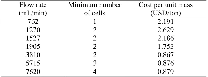
Take that rt 90%, Celec 0.2 USD/kW hr and Ccell 0.1 USD/hr. The least number of flow

Table 2. Number of flow cells and corresponding cost for 90% removal Flow rate

(mL/min)

Minimum number of cells

Cost per unit mass (USD/ton)

762 1 2.191

1270 2 2.629

1527 2 2.186

1905 2 1.753

3810 2 0.867

5715 3 0.876

7620 4 0.879

This study proposed a simple model of an electrochemical flow reactor including fluid flow, mass transport and electrolysis, but the effects of bubble disturbance during the electrolysis or free convection from the change in concentration were neglected. This simulation work, however, can provide useful information for wastewater treatment when a flow system is employed.

5. CONCLUSION

Indium recovery from wastewater is a way to increase the indium resource. This study investigated the indium removal process in an electrochemical flow reactor. The fluid flow, mass transport and electrochemical reactions are considered in the simulation. The simulated results show that the removal performance depends on the flow rate and operation duration. The mass transport performance in a flow system is located between a flow type of cylinder electrode system without rotation and a batch type of a rotating electrode system. The residual indium distribution indicates a two-stage development between the cathode and anode. In the first stage the diffusion layer extends with time while the bulk concentration descends progressively in the subsequent stage. An apparent removal of indium takes place in a short-term operation, but a steady state reached after a long enough operation. At a flow rate of 762 mL/min, the indium removal ratio increases slowly with time while the removal ratio rises quickly at flow rates more than 762 mL/min. However, the saturation level after a short-term incubation is higher at low flow rate than at high flow rate. At 762 mL/min, 90% or more of indium in wastewater can be removed, but only 50% or less of indium can be reduced at 7620 mL/min. When the efficiency is considered in common with the throughput, the operation of the flow reactor can be optimized. Based on energy consumption and equipment cost, two flow cells in series operated at 3810 mL/min may be more economical than a unit cell at any flow rates.

NOMENCLATURE:

A area of electrode, m2

in

A cross-section area of inlet, m2

T

C total cost per unit mass, USD/kg

elec

C electricity price, USD/kW·hr

cell

b

c bulk concentration, mol/m3

i

c concentration of species i, mol/m3

in

c input concentration, mol/m3

out

c output concentration, mol/m3

s

c surface concentration, mol/m3

i

D diffusivity of species i, m2/s d characteristic length, m

E

d distance between anode and cathode, m

B

d distance from cathode to container bottom, m

S

d immersion depth of cathode shaft, m E applied voltage, V

eq

E equilibrium potential, V

T

E total energy consumption, J F Faraday’s constant, C/mol

I current, A

i current density, A/m2 0

i exchange current density, A/m2

m

k mass transfer coefficient, m/s

E

l length of the electrode, m p pressure, N/m2

Q flow rate, m3/s

R universal gas constant, J/mol·K Re Reynolds number

r radial coordinate, m

E

r radius of cathode, m

R

r removal ratio

S

r radius of cathode shaft, m

t

r target removal ratio Sc Schmidt number Sh Sherwood number T temperature, K T Torque, N·m Ta Taylor number t time, s

u velocity, m/s

V volume of electrolyte, m3 z axial coordinate, m

i

z charge number of species i α transfer coefficient

l

f electrical potential of electrolyte, V

s

f electrical potential of electrode, V

h _{overpotential, V}

μ viscosity, kg/m-s

i

ρ density, kg/m3 w rotation speed, rad/s t torque, N-m

1

t characteristic time, s 2

t characteristic time, s

ACKNOWLEDGEMENT

The authors would like to thank the National Science Council, Taiwan, ROC for its financial support (MOST 105-ET-E-002-004-ET) of this study.

References

1. S. Jung, N.G. Park, M.Y. Kwak, B.O. Kim, K.H. Choi, Y.J. Cho, Y.K. Kim, Y.S. Kim, Optical Materials, 21 (2003) 235.

2. N.D. Popovich, S.S. Wong, S. Ufer, V. Sakhrani, D. Paine, Journal of The Electrochemical Society, 150 (2003) H255.

3. T. Minami, Thin Solid Films, 516 (2008) 1314.

4. J. Bandara, P.T. Wansapura, S.P.B. Jayathilaka, Electrochimica Acta, 52 (2007) 4161.

5. Y.-T. Cheng, J.-J. Ho, C.-K. Wang, W. Lee, C.-C. Lu, B.-S. Yau, J.-L. Nain, S.-H. Chang, C.-C. Chang, K.L. Wang, Applied Surface Science, 256 (2010) 7606.

6. H.-K. Kim, J. Jeong, K.-H. Choi, S.-W. Jeong, J.-W. Kang, Electrochemical and Solid-State Letters, 12 (2009) H169.

7. W.-L. Chou, C.-T.Wang, Kai-Yu Huang, Journal of Hazardous Materials, 167 (2009) 467. 8. H.-M. Liu, C.-C.Wu, Y.-H. Lin, C.-K. Chiang, Journal of Hazardous Materials, 172 (2009) 744. 9. L. Zhan, F. Xia, Q. Ye, X. Xiang, B. Xie, Journal of Hazardous Materials, 299 (2015) 388. 10. J. Li, S. Gao, H. Duan, L. Liu, Waste Management, 29 (2009) 2033.

11. K. Takahashi, A. Sasaki, G. Dodbiba, J. Sadaki, N. Sato, T. Fujita, Metallurgical and Materials Transactions A, 40 (2009) 891.

12. H. Hong, H. Jung, S.-J. Hong, Research on Chemical Intermediates, 36 (2010) 761.

13. B.B. Adhikari, M. Gurung, H. Kawakita, K. Ohto, Chemical Engineering Science, 78 (2012) 144. 14. H.N. Kang, J.-Y. Lee, J.-Y. Kim, Hydrometallurgy, 110 (2011) 120.

15. S. Virolainen, D. Ibana, E. Paatero, Hydrometallurgy, 107 (2011) 56. 16. J. Yang, T. Retegan, C. Ekberg, Hydrometallurgy, 137 (2013) 68.

17. W.-S. Chou, Y.-H. Shen, S.-J. Yang, T.-C. Hsiao, L.-F. Huang, Environmental Progress & Sustainable Energy, 35 (2016) 758.

18. Y. Li, Z. Liu, Q. Li, Z. Liu, L. Zeng, Hydrometallurgy, 105 (2011) 207.

19. L. Rocchetti, A. Amato, V. Fonti, S. Ubaldini, I. De Michelis, B. Kopacek, F. Vegliò, F. Beolchini, Waste Management, 42 (2015) 180.

20. B. Swain, C. Mishra, H. S. Hong, S.-S. Cho, Waste Management, 57 (2016) 207. 21. J.-C. Park, Bulletin of the Korean Chemical Society, 32 (2011) 3796.

22. J. Jiang, D. Liang, Q. Zhong, Hydrometallurgy, 106 (2011) 165.

23. H. Yoshida, S. Izhar, E. Nishio, Y. Utsumi, N. Kakimori, F. S. Asghari, The Journal of Supercritical Fluids, 104 (2015) 40.

24. J.E.A.M. van den Meerakker, P.C. Baarslag, M. Scholten, Journal of The Electrochemical Society, 142 (1995) 2321.

25. Y. He, E. Ma, Z. Xu, Journal of Hazardous Materials, 268 (2014) 185.

26. S. Lee, S. Y. Lee, B. Swain, S. S. Cho, C. G. Lee, Materials Testing, 58 (2016) 1001.

28. M. A. Lévêque, Annales des Mines, 13 (1928) 201.

29. D. R. Gabe and F. C. Walsh, Journal of Applied Electrochemistry, 13 (1983) 3.

30. Ph. Mandin, C. Fabian and D. Lincot, Journal of The Electrochemical Society, 153 (2006) D40. 31. Ph. Mandin, C. Fabian and D. Lincot, Electrochimica Acta, 51 (2006) 4067.

32. C. T. J. Low, E. P. L. Roberts and F. C. Walsh, Electrochimica Acta, 52 (2007) 3831.

33. E. P. Rivero, P. Granados, F. F. Rivera, M. Cruz, I. González, Chemical Engineering Science, 65 (2010) 3042.

34. R. Holze, Electrochemical Thermodynamics and Kinetics, Springer-Verlag, Berlin Heidelberg (2007).

35. J. S. Newman, Electrochemical Systems, 2nd ed., Prentice Hall, New Jersey (1991).

36. T. Mizushina, The Electrochemical Method in Transport Phenomena, Advances in Heat Transfer, Vol. 7, Academic Press, New York (1971).

37. J. C. Bazan and J. M. Bisang, Journal of Applied Electrochemistry, 34 (2004) 501. 38. F. F. Rivera and J. L. Nava, Electrochimica Acta, 52 (2007) 5868.

39. D. Pletcher and F. C. Walsh, Industrial Electrochemistry, 2nd ed., Blackie Academic and Professional, UK (1993).

40. R. B. Bird, W. E. Stewart and E. N. Lightfoot, Transport Phenomena, 2nd ed., John Wiley and Sons, New York (2002).