Methods
DAG-informed regression modelling,
agent-based modelling and microsimulation
modelling: a critical comparison of methods
for causal inference
Kellyn F Arnold
,
1,2* Wendy J Harrison,
1,2Alison J Heppenstall
1,3†and
Mark S Gilthorpe
1,2†1
Leeds Institute for Data Analytics, University of Leeds, Leeds, UK,
2School of Medicine, University of
Leeds, Leeds, UK and
3School of Geography, University of Leeds, Leeds, UK
*Corresponding author. Leeds Institute for Data Analytics, University of Leeds, Level 11 Worsley Building, Clarendon Way, Leeds, LS2 9NL, UK. E-mail: [email protected]
†
Joint senior authors.
Editorial decision 15 October 2018; Accepted 2 November 2018
Abstract
The current paradigm for causal inference in epidemiology relies primarily on the
evalua-tion of counterfactual contrasts via statistical regression models informed by graphical
causal models (often in the form of directed acyclic graphs, or DAGs) and their
underly-ing mathematical theory. However, there have been growunderly-ing calls for supplementary
methods, and one such method that has been proposed is agent-based modelling due to
its potential for simulating counterfactuals. However, within the epidemiological
litera-ture, there currently exists a general lack of clarity regarding what exactly agent-based
modelling is (and is not) and, importantly, how it differs from microsimulation
model-ling—perhaps its closest methodological comparator. We clarify this distinction by
briefly reviewing the history of each method, which provides a context for their
similari-ties and differences, and casts light on the types of research questions that they have
evolved (and thus are well suited) to answering; we do the same for DAG-informed
re-gression methods. The distinct historical evolutions of DAG-informed rere-gression
model-ling, microsimulation modelling and agent-based modelling have given rise to distinct
features of the methods themselves, and provide a foundation for critical comparison.
Not only are the three methods well suited to addressing different types of causal
ques-tions, but, in doing so, they place differing levels of emphasis on fixed and random
effects, and also tend to operate on different timescales and in different timeframes.
Key words:causal inference, counterfactuals, directed acyclic graphs, agent-based modelling, microsimulation modelling
VCThe Author(s) 2018. Published by Oxford University Press on behalf of the International Epidemiological Association. 243
This is an Open Access article distributed under the terms of the Creative Commons Attribution License (http://creativecommons.org/licenses/by/4.0/), which permits unrestricted reuse, distribution, and reproduction in any medium, provided the original work is properly cited.
doi: 10.1093/ije/dyy260 Advance Access Publication Date: 5 December 2018 Original article
Introduction
Epidemiology, which entails the study of both the distri-bution and determinants of health and disease, is often considered the core science of public health.1Whilst easy
to conceptualize, it nevertheless remains difficult to prac-tise. Population-level health patterns emerge from a com-plex, dynamic, multi-layered system, in which a multitude of different interrelationships operate2; this
sys-tem is commonly referred to in the literature as a ‘com-plex system’, which is characterized by individual heterogeneity and autonomy, interdependence, spillover effects, adaptivity and evolution, feedback and threshold effects.3Individuals move through space and time, inter-acting with and being influenced by other individuals, groups, social, economic and political constraints, and ge-ography—to name but a few. Understanding the impact of individual behaviour and decision-making on popula-tion health trends—so that we are ultimately able to inter-vene to alter them beneficially—necessarily requires a
causalunderstanding of those patterns and processes that
are important, and at which spatial and temporal scales they operate.
The inherent complexity of such a system poses chal-lenges to anyone attempting to model it; identifying and estimating causal effects creates additional challenges. Causation is a concept of which most, if not all, human beings have an intuitive understanding. Nevertheless, it is a complex phenomenon and remains largely inarticulable; despite thousands of years of philosophical discourse, there exists very little consensus as to what it is, how it can be defined4and—perhaps most importantly for researchers— how it can be inferred within practical research applica-tions.5–10 To address this, many methods have emerged across a range of different disciplines, though the current paradigm for causal inference in epidemiology relies
primarily on the evaluation of counterfactual contrasts via statistical regression models informed by graphical causal models (often in the form of directed acyclic graphs, or DAGs) and their underlying mathematical theory.5 However, there have been growing calls for a more plural-istic approach to causal inference in the field,5,6,11 pre-mised on the argument that there are numerous causal scenarios that do not lend themselves to representation by DAGs and subsequent statistical analyses.
Many authors have proposed more widespread adoption of ‘systems approaches’2,3,12–15—a somewhat nebulous
term for a group of methods that may be used to study the nature of systems. In particular, several authors have identi-fied agent-based models (ABMs) as promising tools for causal inference in complex systems, as they provide a framework for the simulation of counterfactuals.15–17 Perhaps due to agent-based modelling having primarily evolved within and been adopted by the ‘softer’ social scien-ces (e.g. sociology, political science), it remains relatively unfamiliar to epidemiological researchers; moreover, there appears to be little clarity regarding what exactly an ABM is (and is not) and, importantly, how it differs from other sim-ulation models. For example, the recent work of Murray
et al.18demonstrated equivalence between the parametric
g-formula (a statistical method based upon graphical model theory) and what the authors referred to as agent-based modelling, though, in actuality, it is more akin to microsi-mulation modelling. Whilst the distinction between ABMs and microsimulation models (MSMs) may seem self-evident to those who regularly use these methods and trivial to those who do not, it does in fact have important implications for how and under which circumstances each may be used, and thus is worth clarifying.
To this end, we seek to elucidate the distinction be-tween microsimulation modelling and agent-based Key Messages
• Microsimulation modelling and agent-based modelling are closely linked methodologically though historically
dis-tinct. The key features of agent-based modelling are agency and agent-to-agent interaction, which produce highly
complex and ‘emergent’ properties.
• Directed acyclic graph (DAG)-based regression modelling directs greatest focus towards modelling mean structures
(i.e. ‘fixed’ effects), whereas simulation approaches embrace complexity by focusing more on ‘random’ structures.
• Microsimulation modelling provides a bridge between DAG-informed regression modelling and agent-based
model-ling, which may be exploited to bring the mathematical robustness of graphical model theory to bear on simulation
approaches.
• Agent-based modelling can provide a complimentary extension to DAG-informed regression methods in order to
deal with scenarios involving greater complexity (e.g. in which the assumption of no ‘interference’ or spillover effects
may be untenable).
modelling for statistically minded researchers who may be relatively unfamiliar with them; moreover, we describe DAG-informed regression modelling for simulation-minded researchers. Because these methods have largely been confined to separate research disciplines, there exists little overlap in the knowledge about them and skills nec-essary for implementing them, despite calls for greater in-tegration2,13,15,17; our paper aims to fill this gap. We begin by briefly explaining each method and its history, and go on to discuss how their separate evolutions have shaped the types of causal questions to which they are well suited to evaluating. We outline the primary philo-sophical and methodological similarities and differences between them, and conclude with a discussion regarding the implications of these similarities and differences for fu-ture causal analyses and opportunities for fufu-ture methodo-logical work.
A brief history of methods
Historical context is key to understanding both the utility and the defining features of a particular method; therefore, we briefly recap the history of each method, with specific attention given to how it evaluates counterfactuals (see
Box 1for an explanation of counterfactuals).
Graphical causal models and the formalization of
counterfactuals
Causal models trace their roots back to 1918, with Sewall Wright’s invention of path analysis.19,20 They also have origins in structural equation models (SEMs), which emerged primarily in the social sciences (e.g. psychology) and represent groups of causally related variables (both ob-served and latent) as systems of simultaneous (linear) equa-tions.21However, both were subsumed at the turn of the
century under the framework of non-parametric causal models by Judea Pearl in his seminal book Causality.22
These models are typically represented graphically as a set of nodes (variables) connected by a set of edges (represent-ing statistical dependencies), although neither the magni-tude nor functional form of these dependencies are implied or constrained.23 A special subset of such graphs— DAGs—are perhaps the most well known.
A DAG is a graphical causal model in which all edges are unidirectional (hence ‘directed’); these directed edges represent direct causal effects. A path is a sequence of edges connecting two nodes, and there may be multiple paths connecting any two nodes. A causal path is one in which all directed edges flow in the same direction, indicat-ing that the statistical dependency that exists between the nodes is causal in nature. Importantly, no causal paths may exist from any node back to itself (hence ‘acyclic’).23,24 A node may be either endogenous (having at least one di-rect cause represented in the DAG) or exogenous (having none), and a DAG may be considered a ‘causal DAG’ if all common causes between any two nodes are represented in the graph.24 A simplified example is given in Figure 1,
showing the hypothesized causal relationships between sex, weight and systolic blood pressure (SBP).
[image:3.612.316.548.658.692.2]DAGs represent a given system as a number of variables connected by a series of causal pathways; combined with parametric assumptions, they may be thought of as repre-senting the presumed data-generating process, i.e. the pro-cess by which any endogenous variable in the system obtains its value. Given the values for all exogenous varia-bles, the value of any endogenous variable can be known. For example, if we knew the value of sex inFigure 1(and assumed it was a causal DAG for ease of illustration, though in reality this is unlikely), we could also know the values of weight and SBP, because weight depends only
Figure 1. Directed acyclic graph (DAG) depicting the hypothesized causal relationships between sex, weight and systolic blood pressure (SBP).
Box 1. A brief explanation of counterfactuals
Counterfactuals
The counterfactual framework states that an event A
may be considered a cause of an event Y if, contrary
to fact, had A not occurred then Y would not have
oc-curred.4 As an example, imagine that an individual,
Alison, is driving to work and comes to a fork in the
road. She chooses to go left, and arrives late for work.
Upset, Alison declares ‘I should have gone right
in-stead!’ What her statement implies is that her decision
to go left at the fork in the road caused her to be late
for work because had she gone right she would not
have arrived late. Of course, there is no way to prove
such a statement, as it would require Alison to
simul-taneously go both left and right and observe the
out-come under each condition (to guarantee that the
ef-fect is not attributable to any other factor that differed
between drives); nevertheless, the scenario
demon-strates the utility of examining causal effects as
coun-terfactual contrasts between two exchangeable units
of analysis—those that are equivalent in every way
ex-cept for the putative causal factor of interest.
upon sex for its value, and SBP in turn depends upon weight and sex.
Whilst identification of individual-level causal effects is generally agreed to be impossible in the real world within a counterfactual framework (i.e. ‘the fundamental problem of causal inference’), identification ofaveragecausal effects is possible and, indeed, forms the basis of a great deal of causal inference.24Randomized–controlled trials (RCTs)— often considered the ‘gold standard’ for demonstrating causality—create exchangeable units of analysis by ran-domly assigning individuals to receive either the putative causal factor of interest or a standard alternative that acts as the reference (e.g. placebo control). Thus, although
indi-vidualswithin the study likely differ with respect to both
measured and unmeasured characteristics that may affect the outcome of interest, randomization ensures that the distribution of such factors is broadly equivalent between the groups so that, on average, the two groups are ex-changeable and thus any difference in average outcomes may be attributed to the hypothesized causal factor.24
DAGs are an incredibly powerful tool for statistical analyses because they provide the foundation for estimat-ing counterfactual quantities from observed data; they have thus found a natural home amongst disciplines in which data collection and statistical analysis are consid-ered paramount (e.g. epidemiology). Creating exchange-able units of analysis is trivial in a well-conducted RCT but more difficult to achieve with non-experimental data in which the putative causal factor of interest is not randomly assigned; simply comparing the average outcomes between those who were or were not exposed to that factor would, in general, not be sufficient for identifying an average causal effect, since the differences in outcomes might be at-tributable to other differences between the groups. However, in principle, identification of a causal effect could be achieved by comparing the outcomes amongst
subgroups for which the distributions of relevant factors
are broadly equivalent. Such subgroups would therefore be referred to asconditionallyexchangeable (or exchangeable conditional on these factors).
The power of graphical model theory is that it provides a way of determining which variables are sufficient for guaranteeing conditional exchangeability for a given DAG, thereby formalizing counterfactual logic and facilitating what has been referred to as the ‘algorithmisation of coun-terfactuals’.25 Briefly, a set of variables is sufficient for guaranteeing conditional exchangeability if conditioning on that set blocks all ‘backdoor paths’ (i.e. spurious paths that induce statistical dependence due to one or more com-mon causes—referred to as ‘confounding’) between the pu-tative causal factor and outcome of interest whilst leaving all causal paths intact.23In practice, this generally involves
creating a regression model for the outcome that includes as covariates both the putative causal factor and a set of variables sufficient for removing bias due to confound-ing.23InFigure 1, for instance, sex confounds the relation-ship between weight and SBP; therefore, if we wished to estimate the total causal effect of weight on SBP, we could estimate the parameters of the following regression model:
SBP¼b0þb1weightþ b2sexþe:
Assuming that the model has been correctly parameter-ized, we are able to interpret ^b1 as the estimated total causal effect of weight on SBP. In other words, for individ-uals of the same sex (i.e. conditionally exchangeable indi-viduals), every unit-difference in weight corresponds to an expected difference in SBP of^b1, on average. DAGs there-fore provide a framework for using traditional statistical methods to estimate counterfactual quantities and average causal effects via the creation of conditionally exchange-able units of analysis.
Microsimulation models, agent-based models and
the simulation of counterfactuals
Microsimulation and agent-based modelling are closely linked methodologically and conceptually though histori-cally distinct, which perhaps obfuscates where they in fact overlap and where they diverge. Both have roots in cellular automata,26 which first emerged in the 1940s and involve simulating the evolution of a collection of coloured cells within a grid at discrete time steps in accordance with a set of rules based on the states of neighbouring cells. From this, MSMs and ABMs evolved separately (primarily in economics and sociology, respectively) as more complex simulation methods; their development and implementa-tion were greatly enabled by the advent of programmable electronic computers. Whereas both methods have been in use for approximately the last half-century—with Orcutt27 frequently credited as one of the founding fathers of the field of microsimulation and Schelling28 for agent-based modelling—the vast increases in computing power realized in the age of technology have rendered early implementa-tions virtually unrecognizable in comparison to their mod-ern counterparts.29–33
In its most basic form, microsimulation is a method for generating micro-level data, typically by combining in-dividual- and aggregate-level datasets (i.e. population syn-thesis)34; this provides an estimated cross-sectional snapshot of a population. This synthetic population may then be statistically analysed to examine associations between its variables (as in ‘traditional’ data analysis) or, perhaps more interestingly, it can provide the foundation
for a dynamic simulation model (either MSM or ABM). Both dynamic MSMs and ABMs simulate the evolution of heterogeneous individuals through time and potentially space. Each individual possesses a set of attributes (e.g. physical, socio-demographic, geographic), which may be updated at discrete time steps; in microsimulation models, in particular, individuals are often defined as belonging to one of a finite number of mutually exclusive and collec-tively exhaustive states (e.g. healthy, sick and dead), and events of interest are modelled as transitions from one state to another that occur according to a set of deterministic and/or stochastic rules (‘transition probabilities’) defined by the modeller.35–37Conceptualized in this way, one may
see parallels between the data-generating process repre-sented by a DAG and the process by which individuals (and their attributes) evolve within the simulations.
Where MSMs and ABMs usually diverge, however, is in the level of complexity in the assumptions each adopts and adheres to regarding the underlying data-generating processes. A defining feature of ABMs—and what often separates them from MSMs—is the presence of interac-tions amongst individuals34; however, the distinction is pri-marily philosophical rather than methodological. Individuals within an ABM are explicitly conceptualized as
agents—i.e. as autonomous, adaptive individuals with
bounded rationality.3 Often this agency manifests in the form of responding to and making decisions influenced by other individuals within the simulation; such agent-to-agent interaction may give rise to what is referred to in the epidemiological literature as ‘interference’, and makes both representation of the scenario as a DAG and subse-quent statistical estimation of causal effects considerably more complex38–40 because the focus is no longer limited
to central locations (i.e. means) but rather the entire distri-bution of values for each variable as dictated by individual-level interactions. Within a standard DAG (e.g.
Figure 1), each variable has a distribution of values across individuals that is determined by the variables that causally precede it; within an ABM, that distribution has an addi-tional within-variable dependency on individual-level rela-tionships. Thus, the data-generating process of an MSM is more easily represented by a DAG (as in Murrayet al.18) than that of an ABM.
The potential of both MSMs and ABMs to evaluate counterfactual scenarios (or ‘what if’ scenarios17) should be immediately apparent. The modeller may alter e.g. one or more transition probabilities (or features of the agent-to-agent interaction, if applicable), cluster effects or some-how fix or limit the values allowable for any attribute, and then allow the effects of such perturbations to play out in the simulation. MSMs and ABMs inherently provide ex-changeable units of analysis, as each simulated run serves
as a counterfactual scenario given that the initial popula-tion remains unchanged.16
How historical differences have informed
philosophical and methodological
differences
Examining the history of each method, as we have done in the previous section, is useful because historical knowledge is integral to understanding why each evolved in the partic-ular discipline(s) it did and thus what types of causal ques-tions it is well suited to addressing. After all, methods are simply tools developed to accomplish some particular objective; it is no coincidence that the three methods considered here have largely evolved in their separate disci-plines. Hernan41 has provided a particularly interesting commentary on DAG-based regression modelling and sim-ulation modelling, framing their differences in terms of their relative reliance on data vs theory—with DAG-informed models being more reliant on data and ABMs more on theory—and thus reflecting the relative value placed on data and theory within the disciplines in which they are typically used. We illuminate additional differen-ces between the three methods that arise from their sepa-rate historical evolutions, including their relative focus on fixed vs random effects, and the timescales and timeframes in which they operate.
Research questions
Due to its historical methodological foundations in the field of medicine, epidemiology (though arguably a social science) has tended to direct greater focus towards causal questions that lend themselves to experimentation, in an attempt to make inferences as independent as possible of theoretical arguments.41Even when experimentation is in-feasible, large quantities of (observational) individual-level data are collected and statistical methods (e.g. regression modelling) are employed with the aim of mathematically controlling for those factors that would typically be con-trolled via experimental manipulation. The recent revolu-tion in graphical model theory has provided a theoretical foundation for causal data analysis that has historically been lacking, but it nevertheless remains that epidemiology is a data-loving science. Consequently, as noted by Hernan,41 minimizing (albeit not eliminating) the role of theory has necessitated addressing narrower causal ques-tions. This is the context in which DAGs have been employed and in which the majority of methodological work is ongoing.42,43 Disciplines such as sociology and psychology, however, tend to be interested in answering broader, more theory-driven questions relating to
phenomena for which data do not exist or may be difficult to measure or quantify (e.g. social norms); the theory-driven, data-generative nature of ABMs makes them more suitable for modelling such contexts. Economics—the pri-mary realm of MSMs—falls somewhere in between, and in-deed the discipline has shown a greater willingness to embrace graphical model-based methods (e.g. instrumental variable analysis44) than some of the ‘softer’ social sciences.
As an illustration of how use of the three methods dif-fers, we consider obesity as a case study. The obesity epi-demic has previously been characterized as containing many features of a complex system2,3,45as well as elements from a wide variety of disciplines (e.g. biology, social pol-icy, economics, psychology, geography, etc.); thus, it offers an ideal context for comparing the methods of interest.
Box 2provides a sample of the stated research objectives for published studies that have examined obesity using DAG-informed regression modelling, microsimulation modelling or agent-based modelling. Examination of Box 2 reveals several interesting distinctions between the meth-ods; it also illustrates the observation by Hernan41 that
DAG-informed regression modelling and agent-based modelling exist along a spectrum according to the relative weights given to data and theory, with microsimulation modelling providing a bridge between them.
The research questions addressed by DAG-informed re-gression modelling in Box 2 tend to be framed in terms of estimating the effect of a specific factor on a specific out-come. The concept of intervention is often implicit in these analyses (e.g. ‘If we were to intervene to alter exposure to early-life persistent organic pollutions, how would this af-fect BMI?’, as in Karlsenet al.59), but may also be explicit, as in Danaeiet al.56In fact, the example of Danaeiet al.56
is particularly enlightening due to its specific use of the g-formula, which—as has previously been noted by Murray
et al.18—is broadly equivalent to microsimulation, because
it effectively simulates the joint distribution of the variables in a DAG that would have been observed had an interven-tion been enacted in which all individuals were exposed to the putative causal factor of interest.46
Researchers using microsimulation modelling tend to exclusively focus on estimating the effect of a specific
pol-icy or interventionon a target outcome and, often,
deter-mining its cost-effectiveness.37,67 Inherent in and integral to these analyses are specific comparisons between alterna-tive intervention programmes. Given its history in the field of economics, it is perhaps unsurprising but nevertheless il-lustrative that microsimulation modelling is used for such analyses, particularly when contrasted with analyses using agent-based modelling.
The explicit evaluation of interventions in microsimula-tion modelling crosses over to agent-based modelling, with
several of the stated research objectives in the third column of Box 2 referring to specific hypothetical policy interven-tions. However, unique to agent-based modelling analyses is their exploration of social phenomena (e.g. economic segregation, social norms) in the simulation framework. Thus, although they share considerable overlap methodo-logically, microsimulation and agent-based modelling are distinct in their underlying purposes and practical utility. Moreover, because agent-to-agent interactions give rise to greater complexity, ABMs often result in highly nonlinear and chaotic states and produce ‘emergent’ properties68;
consequently, ABMs are less suited than MSMs to produc-ing the detailed predictions often required by economists and policymakers, but arguably more suited to modelling naturally complex social phenomena.
Fixed vs random effects
Another—perhaps underappreciated—distinction between DAG-informed regression models and ABMs is their relative focus on fixed vs random effects, which also arises from their distinct historical evolutions. A natural consequence of using DAG-informed regression models is that intense focus is directed towards modelling mean structures and estimating mean (fixed) effects as opposed to evaluating distributional properties and understanding complexity by examining variation and the patterns of nat-ural heterogeneity. Although DAGs describe causal pro-cesses that could potentially manifest in infinitely many (parametric) ways, the use of regression models to interro-gate causal questions and identify average causal effects makes focus on the distributional properties of the varia-bles of interest effectively redundant. Moreover, their mathematical foundation is built on the assumption of no interference or spillover effects, and so the complexity and heterogeneity that define a complex system are often strictly controlled via study design or averaged out and largely overlooked (thereby treated more as a nuisance and mere ‘noise’ than of substantive interest in its own right). However, it is undeniable that there are myriad determi-nants of health and disease—particularly social ones15— that operate on many levels and in a complex fashion, and about which the ‘random’ structures (possibly arising from individual interactions) are of equal, if not greater, impor-tance to the ‘fixed’ structures. Such determinants may be of great interest to epidemiologists, yet statistical model-ling is limited in the insights it can provide into the poten-tial complexity of random structures that contain spillover effects and interference. For these reasons, causal questions involving such complexities have tended to be relegated to the social sciences, in which greater emphasis is placed on theory as opposed to data (i.e. the realm of ABMs).
Box 2. A sample of the stated research objectives for published studies that have examined obesity using
DAG-informed regression modelling (* denotes use of a ‘g-method’46), microsimulation modelling or agent-based modelling
DAG-informed regression modelling Microsimulation modelling Agent-based modelling
‘. . .to estimate the joint effects of
obesity and smoking on all-cause
mortality and investigate whether
there were additive or
multiplica-tive interactions.’47*
‘. . .to establish whether 52-week
refer-ral to an open-group
weight-manage-ment programme would achieve
greater weight loss and
improve-ments in a range of health outcomes
and be more cost-effective than the
current practice of 12-week
referrals.’48
‘To explore the role that economic
seg-regation can have in creating income
differences in healthy eating and to
explore policy levers that may be
ap-propriate for countering income
dis-parities in diet.’49
‘. . .to estimate the independent
causal effects of body mass index
[. . .] and physical activity on
cur-rent asthma.’50*
‘. . .to estimate the expected impact of
the [1-peso-per-litre] tax [on
sugar-sweetened beverages] on body
weight and on the prevalence of
over-weight, obesity and diabetes in
Mexico.’51
‘. . .[to compare] the effects of targeting
antiobesity interventions at the most
connected individuals in a network
with those targeting individuals at
random.’52
‘. . .to study whether weight-related
anthropometrics, changes in BMI
SDS [standard deviation score]
and physical activity at different
ages in childhood are associated
with atopic disease by late
childhood.’53
‘. . .to estimate changes in calorie intake
and physical activity necessary to
achieve the Healthy People 2020
ob-jective of reducing adult obesity
prev-alence from 33.9% to 30.5%.’54
‘. . .[to] simulate how a mass media
and nutrition education campaign
strengthening positive social norms
about food consumption may
poten-tially increase the proportion of the
population who consume two or
more servings of fruits and
vegeta-bles per day in NYC.’55
‘. . .to estimate the 26-year risk of
CHD [coronary heart disease]
un-der several hypothetical weight
loss strategies.’56*
‘To assess the cost-utility of gastric
by-pass versus usual care for patients
with severe obesity in Spain.’57
‘. . .[to explore] the efficacy of a policy
that improved the quality of
neigh-borhood schools in reducing racial
disparities in obesity-related
behav-iour and the dependence of this effect
on social network influence and
norms.’58
‘. . .[to evaluate] the associations
be-tween early-life POP [persistent
or-ganic pollutant] exposures and
body mass index.’59
‘To analyse the cost-effectiveness of
bariatric surgery in severely obese
(BMI ? 35 kg/m2) adults who have
diabetes.’60
‘. . .to examine: a) the effects of social
norms on school children’s BMI
growth and fruit and vegetable (FV)
consumption, and b) the effects of
misperceptions of social norms on
US children’s BMI growth.’61
‘. . .to assess the mediating role of
anthropometric parameters in the
relation of education and
inflam-mation in the elderly.’62
‘To estimate the impact of three federal
policies on childhood obesity
preva-lence in 2032, after 20 years of
implementation.’63
‘. . .to examine the effects of different
policies on unhealthy eating
behaviors.’64
‘. . .to examine differences in the
contribution of obesity measures
to adenoma risk by race.’65
‘To determine the cost-effectiveness of
gastric band surgery in overweight
but not obese people who receive
standard diabetes care.’66
Foundationally, ABMs are theoretically very different from their statistical counterparts; as recognized by Oakes,69 the outcome of interest is primarily the process by which group phenomena emerge. From the (micro-)sim-ulated processes of ABMs, patterns and properties of the system emerge; mean effects may be eventually derived, but the primary focus is on conceptualizing and modelling the system as a whole, and how individualagencyand
het-erogeneity interact to give rise to aggregate patterns.
Although ABMs have seen some use within epidemiology, this is largely confined to the study of infectious diseases70–73
in which there exist clear transmission mechanisms via in-dividual interaction74and in which it is widely recognized
that the effects of interaction are a fundamental part of the causal mechanism and thus cannot be overlooked.38 Although the random effects arising from agent-to-agent interactions in ABMs are absent in MSMs, individuals re-main the central focus of MSMs rather than average pat-terns. This individual-level focus allows the analysis of heterogeneity and distributional properties that might be masked by approaches considering only mean effects.33,37
Timescale and timeframe
There also exists a large divergence between DAG-informed regression modelling and microsimulation/agent-based modelling with regard to how time is incorporated into the analyses—in terms of both scale and frame. Time is an in-herent factor in any causal analysis, though there are infi-nitely many possibilities regarding the scale at which it is conceptualized and modelled. Because all models are abstractions of reality, both the salient features of a system and the frequency at which they are measured and repre-sented are subjective choices that depend on context (and convenience, in the case of data-dependent analyses). For example, individual activity levels might be modelled every few seconds (as recorded by an activity monitor) to discover how exercise relates to heart rate during high-intensity inter-val training. However, such granularity would likely be un-necessary for determining how exercise relates to adipose tissue levels, in which case individual activity levels might be recorded as an average daily, weekly or monthly value; on the other hand, insufficient granularity of timescale (e.g. yearly or bi-yearly averages, or a one-time cross-sectional measurement) could have a detrimental impact on any anal-yses, as the circular feedback loop that occurs—typically on a much smaller timescale—between physical activity and obesity would be masked.
In general, the timescales upon which both methods operate are strikingly different. MSMs and ABMs tend to model much smaller timescales (e.g. days, weeks, months) than do statistical models because these are closer to the
timescales upon which human behaviour and interactions generally operate, and upon which the effects of policy inter-ventions might be realized. For ABMs in particular, in which agent-to-agent interactions are integral to the causal processes operating (e.g. for infectious diseases), modelling geolocation with high frequency is essential. Greater granularity of time-scale enables the accumulation of emergent properties— although modelled in discrete time steps—to be approxi-mately smoothed. Moreover, abstraction to larger scales has the potential to miss out on the complexity that these models seek to explore and/or explain and, because they are not as limited by data availability, they are able to explore phenom-ena in such granularity when the context requires it. Although DAG-based regression models are theoretically able to model such small timescales, their reliance on data (which tend to be collected infrequently, as in observational health studies, for instance) limits this in practice; they tend to be parameterized in a less granular fashion, which additionally serves their fo-cus on mean effects and model parsimony.
Additionally, the timeframes in which the different mod-els operate diverge. Because they are reliant upon data, DAG-based regression models exclusively model past events; the counterfactuals created are thus thought experiments about whatwould have happenedhad some condition been different. However, public health and epidemiological researchers are generally interested in estimating causal effects because they wish to intervene to alter (ideally benefi-cially) future health states; they may extrapolate the results of their statistical models to infer that whatwould have
hap-penedin the past is equivalent to whatwouldhappen in the
future, but they do not explicitly model this. In contrast, MSMs and ABMs may be used to model both past and fu-ture events by utilizing and synthesizing historical data and estimates to make decisions about hypothetical future inter-ventions; indeed, estimating the future impact of potential policy interventions has historically been fundamental to the utility of these methods.33,37,75
Discussion
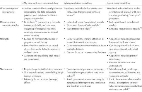
The identifying features of each of DAG-informed regression modelling, microsimulation modelling and agent-based modelling are briefly summarized inTable 1; we also include concise summaries of their accepted strengths and weakness.
As have previously been detailed, there exist substan-tive historical, theoretical and methodological
differen-ces between DAG-informed regression modelling,
microsimulation modelling and agent-based modelling that make them suited to addressing different types of causal questions. DAG-informed regression modelling is ap-propriate for analyses in which the query of interest can be
explicated in the traditional language of ‘exposures’ and ‘outcomes’ (e.g. ‘What is the effect of gastric bypass surgery [the exposure] on risk of diabetes [the outcome]?’), for which sufficient individual-level data are available on a suit-able timescale for the causal processes of interest, and for which spillover effects and interference are thought to be negligible. Moreover, in terms of their practical utility in policy-making decisions, they are better suited to evaluating exposures/interventions whose effects can be safely assumed to be more or less transportable across time, so that the effects estimated from past data may be carried forward to the hypothetical future. When such conditions are met, DAG-informed approaches provide a robust method for causal inference whilst requiring relatively few assumptions, and offer a transparent means for communicating those assumptions.
At the other end of the spectrum, ABMs provide a means for modelling greater complexity—e.g. in the form of indi-vidual interactions and spillover effects—though they do so by requiring a greater number of assumptions. Moreover, because they model scenarios in which key variables of inter-est may not lend themselves to numerical representation, or
in which observed data are not sufficiently granular in time-scale to fully inform parameterization and/or enable effective validation, ABMs inherently contain greater uncertainty about the validity of their causal effect esti-mates.77,79,80 Here, MSMs offer a useful halfway house: they may be able to utilize the robust foundations of graphi-cal causal models and also explore the effects of potentially complex interventions that occur over prolonged periods of time, possibly in the future. The results of Murrayet al.18,81 (which demonstrate equivalence between the g-formula and microsimulation, and use the g-formula to inform microsi-mulation model parameters) represent the first endeavours to bring the mathematical robustness of graphical model theory to bear on simulation approaches. Further methodo-logical research in this area promises to be fruitful.
Funding
This work was supported by the Economic and Social Research Council (ES/J500215/1 to K.F.A.) and the Higher Education Funding Council for England.
[image:9.612.63.549.100.414.2]Conflict of interest:None declared.
Table 1.Brief summaries of the key features, strengths and weakness of each of DAG-informed regression modelling,
microsi-mulation modelling and agent-based modelling. Note that the lists of strengths and weaknesses is not intended to be
exhaustive
DAG-informed regression modelling Microsimulation modelling Agent-based modelling
Short description/ key features
Variables connected by causal pathways representing the data-generating process; used to inform statistical (regression) models
Simulated individuals that evolve over time, often transitioning between ‘states’
Simulated individuals that evolve over time and interact with one another, producing ‘emergent’ properties
Other common names/examples
• G-methods76(parametric g-formula,
inverse probability of treatment weighting of marginal structural models, g-estimation of structural nested models)
• Individual-based (simulation) models
• First-order Monte Carlo models77
• State transition models37
• Individual-based (simulation)
models
• Dynamic (transmission) models78
Strengths • Backed by formal mathematics of
graphical model theory
• Provide robust estimates of causal
effects for clearly defined exposures and outcomes
• Assumptions underlying each model
are transparent
• Can evaluate the (future) effects of
al-ternate intervention strategies
• Can combine parameter estimates from
multiple datasets
• Greater focus on outcome distributions
• Capable of modelling feedback
loops and spillover effects
• Can incorporate
hard-to-mea-sure concepts and individual agency
• Capable of modelling future
timeframes
• Greater focus on outcome
distributions Weaknesses • Require large individual-level datasets
• Not naturally suited to modelling
longi-tudinal scenarios
• Primarily focus on mean (average)
effects
• Combination of parameter estimates
from different populations may result in bias18
• Small parameterization errors may be
perpetuated throughout the simulation and result in large biases
• Model complexity makes
pa-rameterization, calibration and validation difficult
• Lack of consensus about
funda-mental assumptions or under what circumstances causal effect estimates are valid16
References
1. Rothman KJ. Epidemiology: An Introduction. New York:
Oxford University Press, 2002.
2. Galea S, Riddle M, Kaplan GA. Causal thinking and complex sys-tem approaches in epidemiology.Int J Epidemiol2010;39:97–106. 3. Hammond RA. Complex systems modeling for obesity research.
Prev Chronic Dis2009;6:A97.
4. Beebee H, Hitchcock C, Menzies P (eds).The Oxford Handbook
of Causation, 1st edn. New York: Oxford University Press, 2009.
5. Krieger N, Davey Smith G. The tale wagged by the DAG: broad-ening the scope of causal inference and explanation for epidemi-ology.Int J Epidemiol2016;45:1787–808.
6. Vandenbroucke JP, Broadbent A, Pearce N. Causality and causal inference in epidemiology: the need for a pluralistic approach.
Int J Epidemiol2016;45:1776–86.
7. Daniel RM, De Stavola BL, Vansteelandt S. The formal ap-proach to quantitative causal inference in epidemiology: mis-guided or misrepresented?Int J Epidemiol2016;45:1817–29. 8. VanderWeele TJ. On causes, causal inference, and potential
out-comes.Int J Epidemiol2016;45:1809–16.
9. Robins JM, Weissman MB. Counterfactual causation and street-lamps: what is to be done?Int J Epidemiol2017;27:27. 10. Pearl J. Comments on: the tale wagged by the DAG. Int J
Epidemiol2018;43:1002–4.
11. Krieger N, Davey Smith G. Reply to Pearl: Algorithm of the truth vs real-world science (letter).Int J Epidemiol2018;47:1004–6. 12. Green LW. Public health asks of systems science: to advance our
evidence-based practice, can you help us get more practice-based evidence?Am J Public Health2006;96:406–09.
13. Ness RB, Koopman JS, Roberts MS. Causal system modeling in chronic disease epidemiology: a proposal.Ann Epidemiol2007;
17:564–68.
14. Luke DA, Stamatakis KA. Systems science methods in public health: dynamics, networks, and agents. Annu Rev Public
Health2012;33:357–76.
15. Fink DS, Keyes KM, Cerda´ M. Social determinants of population health: a systems sciences approach.Curr Epidemiol Rep2016;
3:98–105.
16. Marshall BD, Galea S. Formalizing the role of agent-based modeling in causal inference and epidemiology.Am J Epidemiol
2014;181:1–9.
17. Auchincloss AH, Diez Roux AV. A new tool for epidemiology: the usefulness of dynamic-agent models in understanding place effects on health.Am J Epidemiol2008;168:1–8.
18. Murray EJ, Robins JM, Seage GR III, Freedberg KA, Hernan MA. A comparison of agent-based models and the parametric g-formula for causal inference.Am J Epidemiol2017;186:131–42. 19. Wright S. On the nature of size factors.Genetics1918;3:367–74. 20. Wright S. The method of path coefficients.Ann Math Stat1934;
5:161–215.
21. Tu YK. Directed acyclic graphs and structural equation model-ling. In: Tu YK, Greenwood DC (eds).Modern Methods for
Epidemiology. Dordrecht: Springer, 2012, pp. 191–203.
22. Pearl J. Causality: Models, Reasoning, and Inference. New York: Cambridge University Press, 2000.
23. Pearl J, Glymour M, Jewell NP.Causal Inference in Statistics: A
Primer, 1st edn. Chichester: John Wiley & Sons Ltd, 2016.
24. Hernan MA, Robins JM. Causal Inference. Boca Raton:
Chapman & Hall/CRC, 2018.
25. Pearl J. The algorithmization of counterfactuals.Ann Math Artif
Intell2011;61:29–39.
26. von Neumann J. The general and locial theory of automata. In: Jeffress LA (ed).Cerebral Mechanisms in Behavior: The Hixon
Symposiom. Oxford: Wiley, 1951, pp. 1–41.
27. Orcutt GH. A new type of socio-economic system.Rev Econ Stat1957;39:116–23.
28. Schelling TC. Dynamic models of segregation.J Math Sociology
1971;1:143–86.
29. Butland B, Jebb S, Kopelman P et al. Foresight: Tackling
Obesities: Future Choices—Project Report, 2nd edn; London:
Government Office for Statistics, 2007.
30. Heppenstall AJ, Evans AJ, Birkin MH. Genetic algorithm opti-misation of an agent-based model for simulating a retail market.
Environ Plann B Plann Des2007;34:1051–70.
31. Manley E, Cheng T, Penn A, Emmonds A. A framework for simulat-ing large-scale complex urban traffic dynamics through hybrid agent-based modelling.Comput Environ Urban Syst2014;44:27–36. 32. Crooks A, Croitoru A, Lu X, Wise S, Irvine JM, Stefanidis A.
Walk this way: improving pedestrian agent-based models through scene activity analysis.Int J Geo-Information2015;4:1627–56. 33. Zaidi A, Rake K.Dynamic Microsimulation Models: A Review
and Some Lessons for SAGE. London: The London School of
Economics, 2001.
34. Lovelace R, Dumont M.Spatial Microsimulation with R. Boca Raton: Taylor & Francis Group, LLC, 2016.
35. Crooks AT, Heppenstall AJ. Introduction to agent-based model-ling. In: Heppenstall AJ, Crooks AT, See LM, Batty M (eds).
Agent-Based Models of Geographical Systems, 1st edn.
Dordrecht: Springer, 2012, pp. 85–105.
36. Sonnenberg FA, Beck JR. Markov models in medical decision making: a practical guide.Med Decis Making1993;13: 322–38.
37. Siebert U, Alagoz O, Bayoumi AMet al. State-transition model-ing: a report of the ISPOR-SMDM modeling good research prac-tices task force-3.Value Health2012;15:812–20.
38. Halloran ME, Struchiner CJ. Causal inference in infections dis-eases.Epidemiology1995;6:142–51.
39. Tchetgen Tchetgen EJ, VanderWeele TJ. On causal inference in the presence of interference.Stat Methods Med Res2012;21:55–75. 40. Ogburn EL, VanderWeele TJ. Causal diagrams for interference.
Stat Sci2014;29:559–78.
41. Hernan MA. Invited Commentary: Agent-based models for causal inference—reweighting data and theory in epidemiology.
Am J Epidemiol2015;181:103–05.
42. VanderWeele TJ.Explanation in Causal Inference: Methods for
Mediation and Interaction, 1st edn. New York: Oxford
University Press, 2015.
43. Burgess S, Timpson NJ, Ebrahim S, Davey Smith G. Mendelian randomisation: where are we now and where are we going?Int J
Epidemiol2015;44:379–88.
44. Angrist JD, Krueger AB. Instrumental variables and the search for identification: from supply and demand to natural experi-ments.J Econ Perspect2001;15:69–85.
45. Diez Roux AV. Integrating social and biologic factors in health research: a systems view.Ann Epidemiol2007;17:569–74.
46. Robins JM, Hernan MA. Estimation of the causal effects of time-varying exposures. In: Fitzmaurice G, Davidian M, Verbeke G, Molenberghs G (eds).Longitudinal Data Analysis. Boca Raton: Chapman & Hall/CRC, 2009, pp. 553–99. 47. Banack HR, Kaufman JS. Estimating the time-varying joint
effects of obesity and smoking on all-cause mortality using mar-ginal structural models.Am J Epidemiol2016;183:122–29. 48. Ahern AL, Wheeler GM, Aveyard Pet al. Extended and standard
duration weight-loss programme referrals for adults in primary care (WRAP): a randomised controlled trial.Lancet2017;389:2214–25. 49. Auchincloss AH, Riolo RL, Brown DG, Cook J, Diez Roux AV.
An agent-based model of income inequalities in diet in the con-text of residential segregation.Am J Prev Med2011;40:303–11. 50. Bedard A, Serra I, Dumas Oet al. Time-dependent associations
between body composition, physical activity, and current asthma in women: a marginal structural modeling analysis. Am J
Epidemiol2017;186:21–28.
51. Barrientos-Gutierrez T, Zepeda-Tello R, Rodrigues ER et al. Expected population weight and diabetes impact of the 1-peso-per-litre tax to sugar sweetened beverages in Mexico.PLoS One
2017;12:e0176336.
52. El-Sayed AM, Seemann L, Scarborough P, Galea S. Are network-based interventions a useful antiobesity strategy? An application of simulation models for causal inference in epidemiology.Am J
Epidemiol2013;178:287–95.
53. Byberg KK, Eide GE, Forman MR, Juliusson PB, Oymar K. Body mass index and physical activity in early childhood are associ-ated with atopic sensitization, atopic dermatitis and asthma in later childhood.Clin Transl Allergy2016;6:33.
54. Basu S, Seligman H, Winkleby M. A metabolic-epidemiological microsimulation model to estimate the changes in energy intake and physical activity necessary to meet the Healthy People 2020 obesity objective.Am J Public Health2014;104:1209–16. 55. Li Y, Zhang D, Pagan JA. Social norms and the consumption of
fruits and vegetables across New York city neighborhoods.
J Urban Health2016;93:244–55.
56. Danaei G, Robins JM, Young JG, Hu FB, Manson JE, Herna´n MA. Weight loss and coronary heart disease: sensitivity analysis for unmeasured confounding by undiagnosed disease.Epidemiology
2016;27:302–10.
57. Castilla I, Mar J, Valcarcel-Nazco C, Arrospide A, Ramos-Goni JM. Cost-utility analysis of gastric bypass for severely obese patients in Spain.Obes Surg2014;24:2061–68.
58. Orr MG, Galea S, Riddle M, Kaplan GA. Reducing racial disparities in obesity: simulating the effects of improved education and social network influence on diet behavior.Ann Epidemiol2014;24:563–69. 59. Karlsen M, Grandjean P, Weihe P, Steuerwald U, Oulhote Y, Valvi D. Early-life exposures to persistent organic pollutants in relation to overweight in preschool children. Reprod Toxicol
2017;68:145–53.
60. Hoerger TJ, Zhang P, Segel JE, Kahn HS, Barker LE, Couper S. Cost-effectiveness of bariatric surgery for severely obese adults with diabetes.Diabetes Care2010;33:1933.
61. Wang Y, Xue H, Chen HJ, Igusa T. Examining social norm impacts on obesity and eating behaviors among US school children based on agent-based model.BMC Public Health2014;14:923. 62. Medenwald D, Loppnow H, Kluttig Aet al. Educational level
and chronic inflammation in the elderly—the role of obesity:
results from the population-based CARLA study. Clin Obes
2015;5:256–65.
63. Kristensen AH, Flottemesch TJ, Maciosek MVet al. Reducing childhood obesity through U.S. federal policy: a microsimulation analysis.Am J Prev Med2014;47:604–12.
64. Zhang D, Giabbanelli PJ, Arah OA, Zimmerman FJ. Impact of different policies on unhealthy dietary behaviors in an urban adult population: an agent-based simulation model.Am J Public
Health2014;104:1217–22.
65. Murphy CC, Martin CF, Sandler RS. Racial differences in obe-sity measures and risk of colorectal adenomas in a large screen-ing population.Nutr Cancer2015;67:98–104.
66. Wentworth JM, Dalziel KM, O’Brien PEet al. Cost-effectiveness of gastric band surgery for overweight but not obese adults with type 2 diabetes in the U.S.J Diabetes Complications2017;31:1139–44. 67. Baroni E, Richiardi M.Orcutt’s Vision, 50 Years On. Torino:
Laboratorio Riccardo Revelli, 2007.
68. Batty M. Cities and Complexity: Understanding Cities with
Cellular Automata, Agent-Based Models, and Fractals.
Cambridge: MIT Press, 2005.
69. Oakes JM. Invited Commentary: rescuing Robinson Crusoe.Am
J Epidemiol2008;168:9–12.
70. Marshall BDL, Paczkowski MM, Seemann Let al. A complex systems approach to evaluate hiv prevention in metropolitan areas: preliminary implications for combination intervention strategies.PLoS One2012;7:e44833.
71. Crooks AT, Hailegiorgis AB. An agent-based modeling approach applied to the spread of cholera.Environ Model Software2014;
62:164–77.
72. Kumar S, Piper K, Galloway DD, Hadler JL, Grefenstette JJ. Is population structure sufficient to generate area-level inequalities in influenza rates? An examination using agent-based models.
BMC Public Health2015;15:947.
73. Neubacher D, Furian N, Vossner S. An agent-based approach to reveal the effects of age-related contact patterns on epidemic spread. European Simulation and Modelling Conference. Leicester, UK, 2015.
74. Li Y, Lawley MA, Siscovick DS, Zhang D, Pagan JA. Agent-based modeling of chronic diseases: a narrative review and future research directions.Prev Chronic Dis2016;13:E69.
75. Siebert U. The role of decision-analytic models in the prevention, diagnosis and treatment of coronary heart disease.Z Kardiol
2002;91:144–51.
76. Naimi AI, Cole SR, Kennedy EH. An introduction to g methods.
Int J Epidemiol2017;46:756–62.
77. Koerkamp BG, Weinstein MC, Stijnen T, Heijenbrok-Kal MH, Hunink MGM. Uncertainty and patient heterogeneity in medical decision models.Med Decis Making2010;30:194–205. 78. Pitman R, Fisman D, Zaric GS et al. Dynamic transmission
modeling: a report of the ISPOR-SMDM modeling good re-search practices task force-5.Value Health2012;15:828–34. 79. Diez Roux AV. Invited commentary: The virtual
epidemiologist-promise and peril.Am J Epidemiol2015;181:100–02.
80. Casini L, Manzo G. Agent-based models and causality: a meth-odological appraisal.The IAS Working Paper Series: Linko¨ping University; 2016: 7.
81. Murray EJ, Robins JM, Seage GR IIIet al. Using observational data to calibrate simulation models.Med Decis Making2018;38:212–24.