Analysis of heterogeneity of variance using anome on ln S^2

Rochester Institute of Technology

RIT Scholar Works

Theses

Thesis/Dissertation Collections

5-1-1998

Analysis of heterogeneity of variance using anome

on ln S^2

Casey Volino

Follow this and additional works at:

http://scholarworks.rit.edu/theses

This Thesis is brought to you for free and open access by the Thesis/Dissertation Collections at RIT Scholar Works. It has been accepted for inclusion

in Theses by an authorized administrator of RIT Scholar Works. For more information, please contact

[email protected].

Recommended Citation

Approved by:

ANALYSIS OF HETEROGENEITY OF VARIANCE

USING ANOME ON

In

S2

by

Casey A. Volino

A Thesis Submitted

111

Partial Fulfillment

of the

Requirements for the Degree of

MASTER OF SCIENCE

111

Applied and Mathematical Statistics

Prof.

Edward G. Schilling

(Thesis Advisor)

Prof.

David

R.

Lawrence

Prof.

Donald D. Baker

(Department Head)

GRADUATE STATISTICS

COLLEGE OF ENGINEERING

ROCHESTER INSTITUTE OF TECHNOLOGY

ROCHESTER, NEW YORK

Title

ofThes~:

ANALYSIS OF HETEROGENEITY OF VARlANCE USING ANOME

ON

In

Sj2

I

hereby grant permission to the Walhcc Memorial

Library

of

RlT

tel

reproduce my thesis

in whole or in pan. Any reproducaon

will

not be for

commercial use or profit.

Forward

While

working

at

Corning,

Incorporated,

I

had

the

good

fortune

of

being

able

to

work with several

highly

skilled senior statistical

engineers,

from

whom

I learned

a great

deal

about various statistical

techniques.

One

such

statistician,

Charles

Comer,

introduced

me

to

an article

by

L.

S.

Nelson1

which

succinctly detailed

the technique

of

using

an

analysis-of-variance-type approach

to

detect

variance

heterogeneity. Sometime

later,

when

I

learned

about

the

analysis ofmeans

(ANOME)

technique, I

thought

it

would

be

interesting

to

use

ANOME

to

analyze variance

heterogeneity

and

then

compare

the

results

to the

ANOVA

Abstract

When

nreplicatesare available

from

a

factorial

experiment,

several methods exist

for

testing

the

validity

of

the

assumption of equal variances within

the

"cells"ortreatment

combinations of

the

experiment.

A

new

test

is

proposed

for

variances of random samples

believed

to

be from

normal populations.

This

new

test

combines

both

the

familiar

graphical

analysis ofmeans

for

treatment

effects

(ANOME)

and

the

analysis of the

logarithms

of

the

within-group

variances

to

produce a graphical

display

of

the test

for

variance

homogeneity.

To

determine

robustness of

the

proposed

test

against

departures from

the

underlying

normality

assumption,

this

new

test

is

also evaluated

for

non-normalpopulations.

Another

analysis-of-means-type

test

was

developed

by

Wludyka

and

Nelson

which

utilizes

Dirichlet

distributions

and

specially

constructed

tables.

The

new

test,

proposed

herein,

has

an advantage

in

that

it

relies

solely

on critical values

developed

for

the

analysis-of-means procedure.

As

an added

simplification,

only

those

critical values

corresponding

to

infinite degrees

of

freedom

arerequired.

A

In

ANOME

analysisof

Nelson's

data (used

to

demonstrate

the

In

AN

OVA

procedure)

yielded

the

same conclusion.

Also,

simulationresults

indicate

that

whenthe

underlying

assumption of

normality is

not

feasible,

the

In

ANOME

procedure

demonstrated

equivalentor superior

Type-I

error-rate

stability

and power

among

tests

which

rely

on

that

assumption.

However,

when

the

underlying

assumption of

normality is tenable, Bartlett's

test

performs

the

best

of all

homogeneity-of-variance

tests

studied

in

maintaining

stable

Type-I

errors and power.

Table

of

Contents

Page

I.

Introduction

1

II.

ANOME

of

In

S2

3

Decision Limits

for ANOME

3

Procedure for ANOME

on

In

S2

4

Example

of

ANOME

on

In

S2

7

III.

Bartlett

&

Kendall's In ANOVA Test

of

Homogeneity

of

Variance

14

IV.

Bartlett's Test

of

Homogeneity

of

Variance

15

V.

Levene's Test

with

Brown

and

Forsythe's Modification

16

VI.

Monte Carlo Simulations

18

VII.

Simulation Results

22

VIII.

Summary

and

Conclusions

29

IX.

Future Work

30

X.

References

32

XI.

Appendix

A-l

34

Exact Factors

for

One-Way

Analysis

of

Means,

Ha

34

XII.

Appendix

A-2

35

Sidak Factors

for

Analysis

of

Means

for

Treatment

Effects,

ha

35

XIII.

Appendix

A-3

36

Example

of

Generating

Random Numbers

(Two-Parameter

Weibull)

36

XIV.

Appendix

A-4

38

Visual

Basic

Subroutines

for Simulations in

Excel

38

XV.

Appendix

A-5

43

Type-I Error Rates

for ANOVA

43

List

of

Tables

Page

Table

1.

Cases

Used For Monte

Carlo

Simulation

18

Table 2.

Results for

Case

1,

Normal Distribution

with

|i

50,

and

a

=

15

22

Table 3.

Results

for

Case

2,

Weibull Distribution

with

CO

=

1,

_and

<|)

=

1.5

24

Table 4.

Results for Case

3,

Gamma Distribution

with

\\f

=

2.5,

and

X

2

25

Table 5.

Results

for

Case

4,

Normal Distribution

with

|I

=

50,

and

c,

=

a,

=

... =

ak.,

=

15,

ak

=

20

25

Table 6.

Results

for Case

5,

Normal Distribution

with

|1

=

50,

and

a,

=

a,

=

... =

ak_,

=

15,

ak

=

30

26

Table 7.

Results for

Case

6,

Weibull Distribution

with

(0=1,

andCp)=

1.5

(First k-1

groups),

CO

=

2

(k*

subgroup)

27

Table 8.

Results

for

Case

7,

Gamma Distribution

with

\|/

=

2.5,

and

A.

=

2

(First k-1

groups),

\\f

-

5.0

(kIh

subgroup)

28

Table A-l. Exact Factors for

One-Way

Analysis

of

Means, Ha

34

List

of

Figures

Page

Figure

1. Example

of

ANOME

on

In

S2

14

Figure 2. Normal

Distributions

Used for Simulations

19

Figure 3. Weibull

Distributions

Used

for

Simulations

20

Figure 4.

Gamma

Distributions Used for Simulations

20

Figure 5. Types

of

Error

in

Hypothesis

Testing

21

Introduction

In

many

statistical

analyses,

the

statistician

is

interested in

testing

the

hypothesis

of

homogeneity

of variances of

two

ormore populations.

Often

these

populations represent

the

"groups"

in

an analysis of

variance,

and

it

is

desirable

to test the

validity

of

the

assumption of equal

"wi

thin-group"

variances.

However,

at

times,

we are

interested

in

only

a

direct

comparison of

the

variability,

or

spread,

among

several candidatepopulations

(i.e.

suppliers,

measurement

devices,

etc.).

In

the

latter

situation,

the

variancescan

be

thought

of

asthose of random samples

from

populationsrepresented

by

the

"groups"

or cells

in

a one

way

or

higher

analysis ofvariance.

Hence,

our

discussion

will

focus

on

the

general case of

variances of random samples

from

populations

constituting

the

"groups"or "cells"

in

the

analysis ofvariance.

Suppose

we

have

a sampleof n observations

from

each of

k

populations.

We

shall

denote

the

random sample

from

population

i

by

{Y;i,

Y,,,

..

.,

Yin}

with samplemean

n

Y,

=-(1)

and sample variance

(Y3-Yi)S

s.2=^-Then

the

hypothesis

we would wish

to test

would

be

of

the

form

H0:

a2

=a22=-=

al,

where

C^

represents

the

variance of

the

ithpopulation.

We

would

then test this

against

the

alternate

hypothesis

HA: Not

Hn

for

at

least

one

O?

.

(4)

xo

When

these

populationsare

thought to

be

normally

distributed,

there

exist several

well-established

techniques

commonly

accepted as appropriate

tests

of

this

hypothesis.

Among

these

are

the

common

F-test

(for

two

variances),

and

Bartlett's

test.

An

approximate

test,

presented

by

Bartiett

and

Kendall3,

involves

performing

the

usual analysis of variance on

the

logarithms

of

the

"within-group" sample variances.

Bartiett

and

Kendall

point out

that the

variance of

In

S2

is independent

of

G2,

and

that

a

known

theoretical

error

term

is

available which

depends

on

only

the number of

replicates, n,

for

each

treatment

combination.

An

approximation

to this

theoretical error

term

given

by

L. S.

Nelson1

is

of

the

following

form:

Var(lnS2),-^

(5)

A

more precise approximation of

this

error

term

is

given

by

Wludyka

and

Nelson2 as

2

2

4

16

Var(lnS2)=

+

-+

r

(6)

v

n-1

(n-1)2 3(n-l)3 15(n-l)5

w

For

n

>

5

replicates per

subgroup,

the

logarithms

of

the

subgroup

variances are

approximately normally

distributed. Thus

the test

ofthenull

hypothesis

in

(3)

above

is

essentially

transformed

into

a

test

on means.

This

test

relieson

the

fact

, as

Scheffe4

indicates,

that

"the

analysis of variance

[procedure]

is

fairly

insensitive

to

the shape of

the

distributions

of

the

estimated

means."

if

we use

loge

(natural

logarithm)

or

log1(l

for

this

test,

since

both

log

functions

are scale

relatedand

ANOVA is

scale

invariant.

For

dealing

with variances

from

non-normal

but

continuous

distributions,

Levene's

test

was modified

by

Brown

and

Forsyfhe7

from

it's

original

form

to

serve as a

non-parametric

test

of variances.

The

proposed procedure

(that does

analysisof means on

the

natural

logarithms

of

the

subgroup

variances)

will

be

compared

to

Bartiett

and

Kendall's

approximate

ANOVA

test,

Bartlett's8

test,

and amodified version of

Levene's

test

due

to

Brown

and

Forsythe. The

comparison will

be

made under

varying

conditions.

ANOME

of

In

S2

Decision Limits

for

ANOME

In

the

usualanalysis of means

for

treatment

effects

(ANOME)

from

a

factorial

experiment,

E. G.

Schilling9

gives

the

following

formula for

the

upper and

lower

decision

limits,

0deha^>

(7)

where

N

=

total

_{number of observations}

in

the

experiment,

k

=

numberofpoints plotted

(number

ofmeans

to

compare).

The

values

for

ha

differ

depending

on whether

the

effectof

interest is

a main effect or an

interaction

effect.

For

main

effects,

the

decision

limits

can

be exactly

specifiedas

h=H-Vrh'

(8)

since

in

the case of

testing

main

effects,

Ha

is

exact.

For interaction

effects,

ha

=

ha

,where

the

ha*

are

Sidak

factors

tabulated

in Table A.9 in E. R. Ott

and

E.

G.

Schilling10,

as

suggested

by

L. S.

Nelson11

Ha

critical values

for

a

=

0.10, 0.05, 0.01,

and

0.001

and

infinite

degrees

of

freedom

are given

in Appendix A-l

.

E. G.

Schilling9

justifies

the

useof

Sidak

factors

with

the

statement,

"For interactions

and nested

factors,

ha*

is

used

because

ofthenatureofthecorrelation

among

points

plotted."

For one-way

layouts,

it

may

by

desirable

for ANOME

on

log-variances

to

be

constructedso that

"effects"

are centered about

their

average

log-variance instead

of about

zero.

One

would

then

be

able

to

easily

retrieve

the

original

subgroup

variances

from

the

"main

effects"

as

S;

=e n

'

.

Procedure

for

ANOME

on

In

S2

To

adapt

the

ANOME

procedure

to the

analysis of

the

logarithms

of

variances,

we

take the

following

steps:

Step

2.

Calculate

the treatment

effects

for

the

main effects as

the

Main Effects for Factor A:

A,=

lnS2 InS2

Main

Effects for Factor B:

B,= lnS2 InS2

(9)

(10)

Repeat

this

for

each

factor in

the

experiment.

Step

3. Calculate

the treatment

effects

for

the

interactions

as

the

difference between

the

average

log-variance for

each

treatment

combination of

the

factors

and

the

grand average of all

the

log-variances,

less any

previously

estimated

lower-order

effects.

(See below for

two-factor

example.)

Interaction Effects for

the

AB Interaction:

AB

= InS2 InS2

A,

B,

(11)

Repeat

this

for

each

interaction in

the

experiment.

Step

4.

Calculate

the theoretical

error

variance,

and

take

it's

square root

for

use

in

computing

the

decision

limits. Regard

this

estimate as

having

infinite

degrees

of

freedom.

Approximation

to the

Theoretical Error Variance.

d>=_2_ +

_2_

+

_!

16_

(12)

e

n-1 (n-1)2

3(n-l)3 15(n-l)5

(!,,

=

Joe

with

degrees

of

freedom

Step

5.

Compute

the

decision limits for

main effects:

Note

that

by

adding

the

average overall mean

back into

the

treatment

effect,

we could

essentially

center

the

effects about

the

overallaverage.

However,

the

decision limits for

the

main effects centered about zero would

be

computed as

follows:

oWirw'

(,3)

whichreduces

to

o.hJ.

(14)

For

a

one-way

analysis,

N

k,

so

the

limits

are given

by

06eHa.

(15)

(N

k

for

a

one-way

analysis,

since after

taking

the

natural

logarithm

ofthe

subgroup

variances,

there

is effectively only

onereplicate per

cell.)

Step

6. Compute

the

decision limits for

interaction

effects

Decision

Limits for Interaction Effects:

The decision limits

for

interaction

effects centered aboutzero are computed

as

follows:

0dXi^'

(16)

where

N

=

total

_{number oftreatmentcombinations}

in

the

experiment,

q

=

degrees

of

freedom

for

the

interaction

effect

tested,

and

The

nextsectionpresentsa worked example

to

further illustrate

the

technique.

Example

of

ANOME

on

In

S2

An

example ofthe

ANOME

on

In

S,2

(henceforth

called

In

ANOME)

procedure

is

nowpresented

using

the

same

data

given

by

L.

S.

Nelson1

to

illustrate ANOVA

on

In S

2.

The

experimental

design involved

three

factors

(A, B,

and

C),

with

k

=

3, 2,

_and

4

levels,

respectively.

The

entire experiment was replicated six

times. The

original

data

is

shown

below.

Al

A2

A3

CI

C2

C3

C4

Bl

B2

Bl

B2

Bl

B2

53.0

49.8

53.0

51.7

51.3

53.2

52.1

53.2

52.5

50.1

48.9

51.9

55.9

51.3

50.4

52.9

51.7

53.1

53.0

52.6

51.5

49.8

53.4

49.6

55.0

51.7

52.6

52.3

52.6

54.1

52.0

53.7

53.5

51.9

50.1

53.1

59.3

52.3

55.0

54.1

51.5

57.5

51.4

56.4

57.0

54.7

56.4

55.0

58.0

53.5

55.6

54.7

51.3

52.3

54.1

54.2

50.3

56.7

49.4

54.1

58.3

53.7

51.4

54.4

55.4

50.8

56.1

51.8

57.5

53.2

53.1

53.1

55.7

55.3

58.9

48.2

57.7

54.3

53.5

55.9

57.0

56.5

61.9

54.6

55.4

54.7

58.0

59.0

49.6

54.7

54.5

54.1

57.7

52.9

57.0

56.7

53.5

55.2

57.3

54.5

56.6

57.6

59.4

59.3

52.2

56.8

56.8

58.1

54.0

59.3

62.0

57.5

57.2

56.8

54.7

59.5

58.5

58.1

62.4

60.3

57.9

55.7

57.9

56.3

63.1

60.9

58.8

56.9

59.7

63.4

56.5

52.3

59.1

58.4

60.8

54.6

60.7

61.0

Step

1.

Compute

the

subgroup

variances,

and

take their

natural

logarithms.

Var(Y)

ln(Var(Y))

Al

Bl

CI

2.544

0.934

Al

Bl

C2

8.944

2.191

Al

Bl

C3

4.819

1.572

Al

Bl

C4

14.942

2.704

Al

B2

CI

2.019

0.703

Al

B2

C2

2.627

0.966

Al

B2

C3

3.391

1.221

Al

B2

C4

2.695

0.991

A2

Bl

CI

1.259

0.230

A2

Bl

C2

8.791

2.174

A2

Bl

C3

5.619

1.726

A2

Bl

C4

3.255

1.180

A2

B2

CI

1.527

0.423

A2

B2

C2

1.335

0.289

A2

B2

C3

14.331

2.662

A2

B2

C4

8.968

2.194

A3

Bl

CI

2.691

0.990

A3

Bl

C2

7.059

1.954

A3

Bl

C3

15.700

2.754

A3

Bl

C4

11.159

2.412

A3

B2

CI

2.508

0.919

A3

B2

C2

5.392

1.685

A3

B2

C3

2.800

1.030

A3

B2

C4

12.603

2.534

Average:

1.518

Step

2.

Calculate

the

treatment effects

for

the

main effects as

the

difference

between

the

average

log-variance

for

each

level

of

the

factor

andthegrand average of allthe

log-variances.

Main Effects

for Factor

A:

A,

=

InS,

InS2

Ai

=

(0.934

₊

2.191

₊

1.572

₊

2.704

₊

0.703

+

0.966

+

1.221

+

0.991)/8

-

1.518

=

-0.108

A2

=

(0.230

+

2.174

+

1.726

+

1.180

+

0.423

+

0.289

+

2.662

+

2.194)/8

-

1.518

= -0.158

Main Effects

for

Factor B:

B,=

lnSj

InS2

Bi

-

(0.934

+

2.191

₊

1.572

+

2.704

+

0.230

+

2.174

+

1.726

+

1.180

+

0.990

+

1.954

+

2.754

+

2.412)/12

-

1.518

=

0.217

B2

=

(0.703

₊

0.966

₊

1.221

+

0.991

+

0.423

+

0.289

+

2.662

+

2.194

+

0.919

+

1.685

+

1.030

+

2.534)/12

-

1.518

=-0.217

Main Effects

for

Factor C:

Cm=lnS^

InS2

C,

=

(0.934

+

0.703

+

0.230

+

0.423

+

0.990

+

0.919)/6

-

1.518

= -0.818

C2

=

(2.191

+

0.966

+

2.174

+

0.289

+

1.954

+

1.685)/6

-1.518

=

0.025

C3

=

(1.572

₊

1.221

₊

1.726

₊

2.662

₊

2.754

₊

1.030)/6

-

1.518

=

0.309

C,

=

(2.704

₊

0.991

₊

1.180

₊

2.194

₊

2.412

₊

2.534)/6

-

1.518

=

0.484

Step

3. Calculate

thetreatmenteffects

for

the

interactions

as

the

difference

between

the

average

log-variance for

each combination of

the

factors

and

the

grand average of all

the

log-variances,

less

any

previously

estimated

lower-order

effects.

Interaction Effects for

the

AB Interaction:

AB

= InS2 InS2

A,

Bf

ABn

=

(0.934

+

2.191

+

1.572

+2.704)/4-

1.518

-(-0.108)

-(0.217)

=

0.223

AB12

=

(0.703

+

0.966

+

1.221

+

0.991)/4

-1.518

-(-0.108)

-(-0.217)

= -0.223

AB2i

=

(0.230

_{+ 2.174+ 1.726+} 1.180)/4-

1.518

-(-0.158)

-(

0.217)

= -0.249

AB22

=

(0.423

₊

0.289

+

2.662

+

2.194)/4

-

1.518

-(-0.158)

-(-0.217)

=

0.249

AB3!

=

(0.990

₊

1.954

₊

2.754

₊

2.412)/4

-

1.518

-( 0.266)

-( 0.217)

=

0.026

AB32

=

(0.919

+

1.685

+

1.030

+

2.534)/4

-

1.518

-( 0.266)

Interaction Effects for

the

AC Interaction:

AC,m=lnS2m

InS2

A,

-Cm

ACn

=

(0.934

₊

0.703)/2

-

1.518

-(-0.108)

-(-0.818)

=

0.226

AC,

2=

(2.191

₊

0.966)/2

-

1.518

-(-0.108)

-( 0.025)

=

0.143

ACB

=

(1.572

₊

1.221)/2

-1.518

-(-0.108)

-(

0.309)

=-0.323

ACu

=

(2.704

₊

0.991)/2

-1.518

-(-0.108)

-(

0.484)

=

-0.047

AC2i

-

(0.230

₊

0.423)/2

-

1.518

-(-0.158)

-(-0.818)

=

-0.215

AC22

=

(2.174

₊

0.289)/2

-

1.518

-(-0.158)

-( 0.025)

=-0.153

AC23

=

(1.726

₊

2.662)/2

-

1.518

-(-0.158)

-( 0.309)

=

0.525

AC2-1

=

(1.180

+

2.194)/2

-1.518

-(-0.158)

-(

0.484)

=-0.157

AC,

=

(0.990

₊

0.919)/2

-

1.518

-( 0.266)

-(-0.818)

=-0.012

AC32

=

(1.954

+ 1.685)/2-

1.518

_{-(0.266) -(0.025)} =

0.010

AC33

=

(2.754

₊

1.030)/2

-

1.518

-( 0.266)

-( 0.309)

=-0.202

AC34

=

(2.412

+

2.534)/2

-

1.518

-(

0.266)

-(

0.484)

=

0.204

Interaction

Effects

for

the

BC

Interaction:

BC,m=lnS2m

InS2

B,

Cm

BCi,

=

(0.934

+

0.230

+ 0.990)/3-

1.518

_{-(0.217) -(-0.818)}=-0.199

BC12

=

(2.191

+

2.174

+

1.954)/3

-

1.518

-( 0.217)

-( 0.025)

=

0.346

BC13

=

(1-572

+

1.726

+

2.754)/3

-

1.518

-( 0.217)

-( 0.309)

=

-0.027

BC14

-

(2.704

+

1.180

+

2.412)/3

-

1.518

-( 0.217)

-( 0.484)

=

-0.121

BC21

-

(0.703

+

0.423

+

0.919)/3

-

1.518

-(-0.217)

-(-0.818)

=

0.199

BC22

=

(0.966

₊

0.289

₊

1.685)/3

-

1.518

-(-0.217)

-( 0.025)

=

-0.346

BC23

=

(1.221

₊

2.662

₊

1.030)/3

-

1.518

-(-0.217)

-(

0.309)

=

0.027

BC24

=

(0.991

₊

2.194

₊

2.534)/3

-

1.518

-(-0.217)

-( 0.484)

=

0.121

Interaction Effects for

the

ABC Interaction:

ABC

=

lnS2m

-InS2

-A,

B,-Cm-AB-AC,m-BC,m

ABCm

=

ABCii2

=

ABC3

=

ABCi,4

=

ABC21

=

ABC122

=

ABC,

23 =

ABC124

=

ABC211

ABC212

=

ABC2,3

=

ABC214

=

ABC221

=

ABC222

ABC223

=

ABC224

=

ABC311

=

ABC3i2

=

ABC3i3

=

ABC3,4

=

ABC321

=

ABC322

-ABC323

=

ABC324

=

(0.934)

-1.518

-(2.191)

-1.518

-(1.572)

-1.518

-(2.704)

-1.518

-(0.703)

-1.518

-(0.966)

-1.518

-(1.221)

-1.518

-(0.991)

-1.518

-(0.230)

-1.518

-(2.174)

-1.518

-(1.726)

-1.518

-(1.180)

-1.518

-(0.423)

-1.518

-(0.289)

-1.518

-(2.662)

-1.518

-(2.194)

-1.518

-(0.990)

-1.518

-(1.954)

-1.518

-(2.754)

-1.518

-(2.412)

-1.518

-(0.919)

-1.518

-(1.685)

-1.518

-(1.030)

-1.518

-(2.534)

-1.518-(-0.108)

-(

(-0.108)

-(

(-0.108)

-(

(-0.108)

-(

(-0.108)-(-(-0.108)

-

(-(-0.108)

-(-(-0.108)

-(-(-0.158)

-(

(-0.158)

-(

(-0.158)

-(

(-0.158)

-(

(-0.158)

-

(-(-0.158)

-

(-(-0.158)

-

(-(-0.158)

-(-(

0.266)

-(

(

0.266)

-(

(

0.266)

-(

( 0.266)

-(

( 0.266)

-

(-( 0.266)

-

(-(

0.266)

-

(-( 0.266)

- (- (0.217)- (-0.217)- (0.217)-

(-0.217)-(-0.217)

-

(0.217)-(-0.217)

-(-0.217)

-(-0.217)

-

(-0.217)-(-0.818)

-(

0.025)

-( 0.309)

-(

0.484)

-

(-0.818)-(

0.025)

-(

0.309)

-(

0.484)

-

(-0.818)-(

0.025)

-(

0.309)

-(

0.484)

-

(-0.818)-(

0.025)

-(

0.309)

-(

0.484)

-

(-0.818)-( 0.025)

-( 0.309)

-( 0.484)

-

(-0.818)-( 0.025)

-(

0.309)

-( 0.484)

-(

0.223)

-(

0.223)

-(

0.223)

-(

0.223)

-(-0.223)

(-0.223)

-(-0.223)

-(-0.223)

-(-0.249)

-(-0.249)

-(-0.249)

-(-0.249)

-( 0.249)

-( 0.249)

-(

0.249)

-(

0.249)

-(

0.026)

-( 0.026)

-( 0.026)

-( 0.026)

-(-0.026)

-(-0.026)

-(-0.026)

-(-0.026)

-0.226)

0.143)-0.323) 0.047)

0.226)

0.143)

0.323)

0.047) -0.215) -0.153)

0.525)

-0.157) -0.215) -0.153)

0.525)

-0.157) -0.012)

0.010)

-0.202)

-0.204)

--0.012)

0.010)

0.202)

0.204)

-(-0.199)

=

(

0.346)

=

-(-0.027)

= -(-0.121) = -(0.199) :

-(-0.346)

=

-(

0.027)

:

-(0.121)

-(-0.199)

:

-(

0.346)

=

-(-0.027)

= -(-0.121) = -(0.199) =

-(-0.346)

=

-(

0.027)

=

-(0.121)=

-(-0.199)=

(

0.346)

=

-

(-0.

027)

(-0.121)

= -(0.199) :

-(-0.346)

=

-( 0.027)

=

Step

4.

Calculate

the

theoreticalerror

variance,

and

take

it's

square root

for

use

in computing

the

decision limits.

Regard

this estimate as

having

infinite degrees

of

freedom.

61=

i-

+

-lT

+

_L^-">

0.4903

6-1

(6-1)2 3(6-l)3 15(6-1)5

6e

=

y[&l =

V0.4903

=

0.70021

Step

5. Compute

the

decision

limits for

main effects

(shown

for

a

0.05).

(k~

Decision

Limits for Main Effects:

0

daH.|

e

aVN

A:

k

=

3

levels,

H

=

Ho.os,

3,~=

1.91,

N

=

24.

Hence,

fk"

I 3

0

a

H

J

=>

0

0.70021*1.91*

J

=>

0

0.4728

VN

V24

B:

k

=

2

levels,

Ha

=

Ho.os,

2,

~ =

1

.386,

N

=

24.

Hence,

fk"

[Y

0

a

=>0+

0.70021* 1.386*

J

=>

010.2801

aVN

V24

C:

k

=

4

levels,

K^

=

Ho.os,

4,~=

2.14,

N

=

24.

Hence,

nr

/

4

0

a

HJ=>0

0.70021*

2.

14*

J

=>00.6116

e

aVN

V24

Step

6. Compute

the

decision

limits

for

interaction

effects

(shown for

OC

=

0.05).

AB:

k

=

3

*

2

=

6

levels,

q

= ab-a-b

+

l

=

6-3-2+l=2,

hlns

c

=2.631,

N

=

24.

Hence,

the

decision limits

are

fa"

HT

0

a

h\

=>0

0.70021*2.631*

J

=>00.5317

e

aVN

V24

AC: k

=

3

*

4

=

12

levels,

q

= ac-a-c+l =

12-3-4+l

=

6,

h005

12M

=

2.858,

N

24.

Hence,

the

decision limits

are

I

n \f\

0

+

ah*

p-

_=>

₀

0.70021

*

2.858

*

J

=>

0

1.0003

VN

V24

BC: k

=

2

*

4

=

8

levels,

q

=

bc-b-c

+

l

=

8-2-4+l

=

3,

h005

8,

=

2.727,

N

=

24.

Hence,

the

decision

limits

are

0

6h"

-=>

0

0.70021

*

2.727

*

J

=>

0

+

0.6749

VN

V24

ABC:

k=3*2*4

=

24

levels,

q

= abc- _ab

-ac-

be

+

a

+

b

+

c-

1

=

6,

h005

24oo

3.071,

N

=

24.

Hence,

the

decision limits

are

0

ah' =>0+

0.70021*3.071*

=>0

1.0749

e a^

N

V24

Step

7.

Construct

the

chart.

Note

that

the

chart

(next page)

displays

decision limits

at

the

a

=

0.01

level,

as well as at

the

OC

0.05

level

as calculated above.

As

can

be

seen

from

the

In ANOME

chart,

the

variability

differed for

the

different

levels

of

factor C. In

particular,

wesee

that the

variability for

the

first level

of

factor C is

significantly

less

than

the

variability for

the

other

three

levels

of

factor

C.

[image:22.561.80.490.110.365.2]

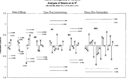
Figure 1: Example

of

ANOME

on

In

S2.

1.5 Main

Effects

0.5

c o

v

E

-1.5

Testof

Homogeneity

ofVariance AnalysisofMeansonInS2

LDLandUDLshownfora=0.05,and a=0.01

Two-Way

Interactions^

Three-Way

Interaction

-1.235 1.075

0 589 0.473

0.746

-fl.612

AC ABC

-0280

Tb

0 280

--0.368

-0473

0.589

BC

A

ft

X

-0.818

-+ _0.612

0.746

^0532 0 635

-0.675

--0.798

>^

I

l-L₀₀

-1.075

-1.235

A, B,andC

Bartiett &

Kendall's

In ANOVA Test

of

Homogeneity

of

Variance

Bartiett

and

Kendall's3

ANOVA-type

test

of

homogeneity

of variance

involves first

computing

the

subgroup

variancesand

then

computing

their

natural

logarithms,

as was

shown

previously

for

the

ANOME

on

In

S

.

Next,

the theoretical

error variance

is

computed

based

on

the

number of replications as shown

in

equation

(12). Then

the

usual sum of

squares,

degrees

of

freedom,

and meansquares are computed

for

every

term

in

the

original

model.

Usually,

we would not

have

an error

term

for

this

situation,

since

there

is

now

effectively only

onereplicate of

the

entire experiment and

the

model wouldtherefore

be

completely

specified.

However,

we make use of

the theoretical

error variance with

infinite

degrees

of

freedom

to

compute values

for

the

F-statistics

andperform

tests

of

hypothesis.

The

analysis of

the

example

data from L. S. Nelson

is

shown

below.

In

ANOVA

on

L. Nelson's Data

Source

DF

Adj

SS

Adj

MS

F

p

0.86224

0.43112

0.87925

0.4151

1.12867

1.12867

2.30188

0.1292

6.00366

2.00122

4.08141

0.0066

**

0.90023

0.45012

0.91800

0.3993

1.26216

0.21036

0.42902

0.8601

1.04869

0.34956

0.71291

0.5441

3.50764

0.58461

1.19229

0.3069

0.49033

Again

wearrive at

the

conclusion

that the

variability differed for

the

different levels

of

factor

C. This

time, however,

further investigation is

required

to

determine

the

nature of

this

difference.

Bartlett's Test

of

Homogeneity

of

Variance

Bartlett's8

test

of

homogeneity

of variance

is

amodification of

Neyman

and

Pearson's12

generalized

likelihood-ratio

test

(LI test, 1931). This

modification

involved

replacing

the

biased

maximum-likelihoodestimators of

the

variances with unbiased

A

2

B

1

C

3

A*B

2

A*C

6

B*C

3

A*B*C

6

Error

oo

estimators and

substituting

n,-l

for n,

in

the

weights.

Bartlett's

test

is

known

to

rely

heavily

on

the

assumptionof

normality

of

the

underlying distributions.

The

value of

the test

statistic

is determined

from

the

data

by

first

computing

the

sample variances of each of

the

k

subgroups and

then

computing

the

subsequent pooled

sample variance as

IK-Ds,2

pooled '='

N-k

(17)

Then

base-10

logarithms

are

taken

of each of

the

k

sample variancesand of

the

pooled

variance.

Ultimately,

the test

statistic

is

given

by

(N-k)log10s^oled-X(ni-l)log10s12

ll

=2.3026

-1

+

-1

(

k

3(k-l)

1

1

trX-i

N-k

(18)

The

valueof

%0

is

then

compared

to the

critical chi-square value with

k-1

degrees

of

freedom.

Levene's Test

with

Brown

and

Forsythe's Modification

Levene's6

test

with

Brown

and

Forsythe's

modification

is essentially

a

non-parametric

test

of

homogeneity

of variance.

The

test

statistic

is

constructedas

follows:

Let

Vii

=

Y

-

Y

y

(19)

where

Y-

the

jthobservation

in

the

ith

group

and

Yj

=

the

_{median of}

the

i' _group.

Then form

the

one-way ANOVA

statistic

Zni(V,-y.)2

i=l

F(calc)

=

k

k~l

,

(20)

si^-v,.)2

N-k

where

%

v.

=

^-(21)

V=J1

,

(22)

j='

N

and

N

=

In,

i=l

(23)

is

the total

number of observations

in

the

experiment.

The

value of

the test

statistic,

F(calc),

is

compared

to

a critical value of

the

F-distribution,

with

k-1

numerator

degrees

of

freedom

and

N-k denominator

degrees

of

freedom.

Monte

Carlo

Simulations

Simulations

providedthemeans

for

assessing,

undercontrolled

conditions,

the

ability

of

these

individual

tests to

reject

correctly

or

incorrectly

the

null

hypothesis. All

simulations

involved

a

balanced,

one-way layout. Seven

cases were

considered,

as

indicated in Table 1

.

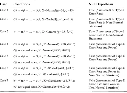
Table

1

Cases Used For Monte Carlo Simulation

Case

Conditions

Null

Hypothesis

Case

1

o"i2= 0"22

Case

2

cm2=

<j2

Ck2

,

X~Normal(p=50,

<7=15)

OV2

,

X~Weibull(CO=l,

<t>=1.5)

Case 3

oV

= a,2= = ak2

^

X~Gamma(\|/=2.5,

A.=2)

Case 4

d2= Q22- - Ok-i2

,

X~Normal(U=50,

0=15)

Ok2_notequal

since,

X~Normal(U=50,

O"=20)

Case 5

<ji2= C22= ...

= Ck-i2

,

X~Normal(Lt=50, C=15)

Ok2_notequal

since,

X~Normal(U=50, O=30)

Case 6

oV

= G22= .. . =

ak-i2

,

X~WeibuU(CO=

1

,

(|)=1.5)

CTk2

notequal

since,

X~Weibull(C0=2,

<p=

1.5)

Case 7

oV

=a22 = .

=OVi2

,

X~Gamma(\|/=2.5,

X-2)

<Jk2_{not equal}

since,

X~Gamma(l|/=5.0,

X.=2)

True

(Assessment

of

Type-I

Error

Rate)

True

(Assessment

of

Type-I

Error Rate

in

Non-Normal

Situations)

True

(Assessment

of

Type-I

Error Rate in Non-Normal

Situations)

False (Assessment

of

Type-II

Error Rate

and

Power)

False (Assessment

of

Type-II

Error Rate

and

Power)

False

(Assessment

of

Type-II

Error Rate

and

Power in

Non-Normal

Situations)

False (Assessment

of

Type-II

Error

Rate

and

Power in

Non-Normal

Situations)

To

assess

the

Type-I

errorrate

in

Cases

1, 2,

and

3,

k

=

2, 4,

6, 8,

and

10

subgroups

weregeneratedand

compared,

withn=

2,

3,

..

.,

10

replicateseach.

The

other

four

cases

assessedthe power of

the

homogeneity

of variance

tests

using

comparisons of

k

=

2, 4, 6, 8,

and

10

subgroups with n =

2, 3,

. . [image:26.561.68.494.221.535.2]

One

thousand

simulations per condition

(case,

subgroup,

and replicate

combination)

were conducted

in

accordancewith

random-number-generating

procedures outlined

by

Dodson

and

Nolan13

These

procedures make use of

the

fact

that

all

BASIC-type

programming

languages

are capable of

producing

uniformly-distributed pseudo-random

numberson

the

[0,

1]

interval. These

uniformly-distributedrandom numbers can

be

used

to

generate other random numbers

for

almost

any distribution. In

the

simplest

form

of

random-number

generation,

this

is done

by

setting

the

cumulative

distribution function

of

the

desired

density

function

equal

to the

uniformly-distributed random number andthen

solving

for

the random variable of

the

new

distribution.

An

example of

this

procedure

for

the

two-parameter

Weibull

distribution is

shown

in

Appendix A-3. When

a closed

form does

not exist

for

the

cumulative

distribution

function,

special algorithms must

be

employed.

Two

such algorithms wereused

to

generate

Normal-distributed

and

Gamma-distributed

random

numbers.

The

code

for

all random numbers generated

is

available

in Appendix A-4.

[image:27.561.144.421.475.657.2]

The

three

Normal distributions

chosen

for

this

study

areshown

in Figure 2.

Figure 2: Normal Distributions Used for Simulations

Normal Distributions

90 100

[image:28.561.126.442.129.341.2]

The

two

forms

of

the

Weibull distribution

used

for

simulations are shown

in

Figure 3.

Figure 3: Weibull

Distributions

Used for Simulations

Weibull Distributions

*=Shape Parameti

01=_ScaleParamete

0)=1 *=1.5

/

v*=15

fix)

= -^x-'e B

\

1.5 2 0 2.5 3.0 3.5

X

The

two

forms

of

the

Gamma

distribution (both

Chi-Square,

in

this

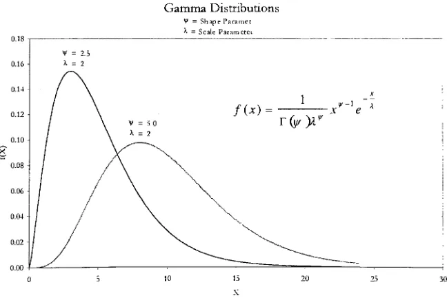
case,

since

A,

2)

are

shown

in Figure 4.

Figure 4:

Gamma Distributions Used for Simulations

Gamma

Distributions

V=ShapeParamec ^=ScaleParanacrei

[image:28.561.120.444.445.663.2]

Once

randomnumbers of

the

appropriate

type

were

generated, the

number of

rejections of

the

null

hypothesis

(out

of one-thousand

simulations)

was recorded

for

eachset

of conditions.

This

was

done concurrently

on

the

data

for

each of

the

following

statistical

tests:

1

.

the

standard

ANOVA for

testing

means,

2.

the

ANOVA

on

In

S,2

(In

ANOVA)

to test

for

homogeneity

of

variance,

3.

the

proposed

ANOME

on

In S

2

(In

ANOME)

to

test

for

homogeneity

of

variance.

4.

Bartlett's Test

of

homogeneity

of

variance,

5.

the

standard

F-test

(for k

=

2

_variances

only),

and

6.

Levene's

test

with

Brown

and

Forsythe's

modification.

In

situations were

the

null

hypothesis

of equal variances was

true,

the tests

were

comparedon

the

basis

oftheir

ability

to

maintain,

over all

conditions,

the expected

Type-I

error rate.

When

the

null

hypothesis

was

false (that

is,

when

the

last

of

k

variances wasnot

equal

to the

other

k-1

variances),

the tests

were compared on

the

basis

of power.

This

is

more

easily

understood

considering

the

following

familiar

diagram:

Figure

5: Types

of

Error

In Hypothesis

Testing

Types

of

Error:

Reject 1 1:

Simulation Conditions

Accept H:

Type-I

Error

a

Correct

Decision

Power

(1-P)

Correct

Decision

Type-II

Error

P

H0

True

H0

False

Casel

Case5

Case6

Case7

Simulation

Results

The

behavior

of

the tests

of

homogeneity

of variance

in conforming

to the

Type-I

error rate at

the

five

percent

level

arepresented

in Tables

2,

3,

and

4. Each

of

the tables that

follow

display

the

number of rejections

(at

the

a

=

0.05

_significance

level)

of

the

null

hypothesis

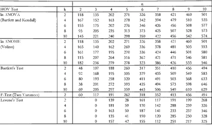
of equal variances out of one-thousand simulations.

Table 2: Results for Case

1,

Normal Distribution

with u=

50,

andO=

15

(Number of

rejections_ofthenull

hypothesis

out

of

1000)

n

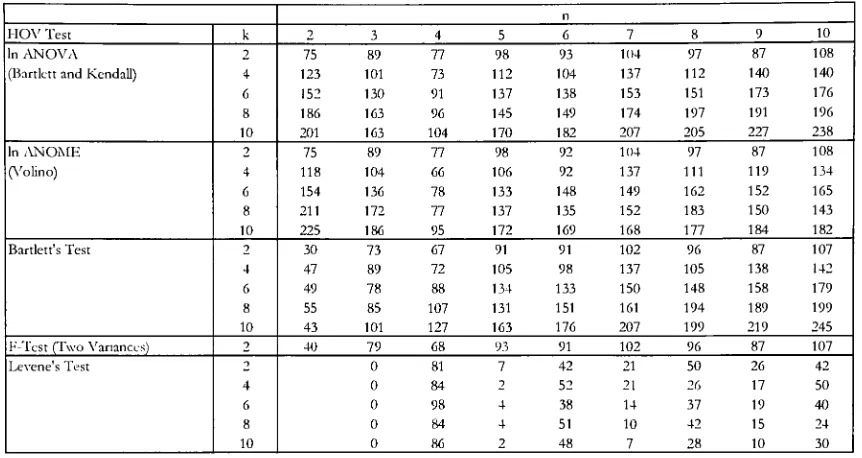
HOVTest k 2 3 4 5 6 7 8 9 10

InANOVA 2 68 35 37 40 53 44 44 50 35

(Bartiettand

Kendall)

4 108 63 47 48 45 46 50 69 71

6 113 65 56 58 45 51 42 47 38

8 120 69 56 46 44 53 57 55 41

10 116 50 55 56 48 51 69 51 69

InANOME 2 68 35 37 40 53 44 44 50 35

(Volino)

4 119 70 50 49 46 52 53 70 66

6 142 82 66 77 54 53 46 65 47

8 172 98 85 66 75 77 67 62 50

10 177 92 93 88 70 72 94 64 76

Bartlett'sTest 2 34 28 35 36 51 40 43 48 35

4 31 39 27 33 38 41 39 54 63

6 36 32 31 41 40 34 33 38 38

8 19 30 26 20 34 34 50 40 33

10 16 21 25 32 28 39 50 39 47

F-Test(Two

Variances)

2 45 30 35 37 51 41 43 48 35

Levene's Test 2 0 49 7 46 9 32 18 33

1 0 59 1 30 9 31 15 40

6 0 55 0 25 10 31 12 23

8 0 50 0 27 6 53 15 17

10 0 58 0 27 6 42 14 36

Even

though the

assumption of approximate

normality

of

In

S2

is

stated

in many

references as

holding

for k

>

5,

the

number of replicates within each cell was examined

for k

<

5,

as well as

k

=

5, 6,

..

.,

10.

In

fact,

"real

world"

experiments

frequendy

have fewer

than

five

replicates.

It

is

of

interest,

therefore,

to

study

the

behavior

of

these

statistics under

less-than-idealconditions.

Both

the

In ANOVA

and

In

ANOME

techniques

are more apt

to

reject

the

hypothesis

of equal variances

than

is

the

F-test,

Bartlett's

test,

or

Levene's

test.

Between

In ANOME

and

In

ANOVA,

as

k

increases,

In

ANOME

rejects

slightly

more often

than

In

ANOVA.

This

makes

In ANOME

in its

present

form less

attractive

than

other

homogeneity-of-variance

tests

for k

>

6

or

7.

Bartlett's test,

given

the

conditionof

normality,

performed closest

to the

expected nominal rejection rate of

50

out of

1000,

or

5%.

Curiously,

in Levene's test,

there

is

a

kind

of

"odd-even"

effect

that

could

be due

to

the

modification of

Levene's6

original

test

by

Brown

and

Forsyfhe7

(Brief

mention of

this

"odd-even"

effect was made

in

Conover, Johnson,

and

Johnson.14)

For

oddnumbers of

replicates,

the

median

is

the value of

the

"middle"observation

in

terms

ofmagnitude.

Considering

deviations

from

the

median,

based

on an odd number of

replicates,

one term

in

equation

(19)

is

always zero.

Hence,

averages of

the

Vtj

are smaller

making

the test

overly

conservative relative

to the

nominal

Type-I

rejection rate.

In

fact,

for

n =

3

_{replicatesper}

cell,

the

null

hypothesis

was never rejected!

(Calculations

from

the

simulation programswere

cross-checked

frequently

withthe results obtained

from

both SAS

and

MINITAB,

and all

test-statistics

andp-values

agreed.) For

an evennumber of

replicates,

the

results

from

Levene's

test

were

less

conservative

than

results

for

oddnumbers of

replicates,

but

were still

below

the

nominal rejection rate of

five

percent.

The

results

for

the

Weibull

and

Gamma

distributions

show

the

dependence

of all of

these

tests,

except

Levene's,

on

the

underlying

assumption of normality.

Type-I

errorrates

for

all

but Levene's test,

whichagain gives evidence of an

"odd-even"

effect,

are at

times

more

than triple

or quadruple

the

norninal

five

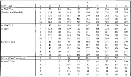
percent rejection rateone would expect.

[image:32.561.66.497.117.346.2]

Table 3: Results for Case

2,

Weibull Distribution

with(0=

1,

and (

(Number of

rejections

of

thenull

hypothesis

out

of 1

000)

1.5

n

ITOVTest k 0 ₃ 4 5 6 7 8 9 10

In ANOVA 2 75 89 77 98 93 104 97 87 108

(Bartiettand

Kendall)

4 123 101 73 112 104 137 112 140 140

6 152 130 91 137 138 153 151 173 176

8 186 163 96 145 149 174 197 191 196

10 201 163 104 170 182 207 205 227 238

InANOME 2 75 89 77 98 92 104 97 87 108

(Volino)

4 118 104 66 106 92 137 111 119 134

6 154 136 78 133 148 149 162 152 165

8 211 172 77 137 135 152 183 150 143

10 225 186 95 172 169 168 177 184 182

Bartlett's Test 2 30 73 67 91 91 102 96 87 107

4 47 89 72 105 98 137 105 138 142

6 49 78 88 134 133 150 148 158 179

8 55 85 107 131 151 161 194 189 199

10 43 101 127 163 176 207 199 219 245

F-Tcst (Two

Variances)

2 40 79 68 93 91 102 96 87 107

Levene'sTest n _{0 81 7 42 21 50 26 42}

4 0 84 ? _{52 21 26 17 50}

6 0 98 4 38 14 37 19 40

8 0 84 4 51 10 42 15 24

10 0 86 2 48 7 28 10 30

For

tests

of equal variances

in

non-normal

situations,

only Levene's test, for

even

numbers of

replicates,

yieldeda

Type-I

rejection rate comparable

to the

nominal

5%

rate.

All

other

tests

resulted

in greatly inflated Type-I

errorrates relative

to the

nominal.

In

the

case

of an

underlying Weibull

distribution,

In

ANOME

was comparable

to

or

better

than

In

ANOVA

and

Bartlett's

Test for

n

>

4

replicatesper subgroup.

Also,

as

the

number of

variances,

k, increased,

In ANOME

showed

slightly better Type-I

error rate

stability

than

did

either

In ANOVA

or

Bartlett's Test.

[image:33.561.65.486.92.330.2]

Table 4: Results for Case

3,

Gamma Distribution

with\(/=

2.5,

and

X

=

2

(Number of

rejections

of

thenull

hypothesis

out

of

1000)

n

HOVTcst k 2 3 4 5 6 7 8 9 10

InANOVA 2 88 75 89 105 109 116 117 139 127

(Bartiettand

Kendall)

4 114 98 122 134 139 154 165 181 185

6 160 130 125 177 186 217 233 207 228

8 170 135 163 188 210 223 253 262 278

10 184 134 162 199 224 263 289 306 312

In ANOME 2 88 75 88 105 109 116 117 139 127

(Volino)

4 129 95 124 122 129 132 157 165 178

6 184 125 139 157 154 203 202 188 210

8 186 153 158 182 178 205 9->a 222 254

10 220 164 162 176 172 224 233 233 254

Bartlett's Test 2 49 61 83 99 103 111 112 134 122

4 58 84 110 124 139 156 165 180 187

6 63 103 115 176 197 231 232 225 234

8 68 111 170 204 217 246 277 292 286

10 67 124 195 232 242 283 315 329 329

F-Test(Two

Variances)

2 59 67 84 99 104 111 112 134 122

I.cvcnc'sTest n _{0 82 5 46 24 38 29 49}

4 0 109 5 44 15 43 19 43

6 0 98 7 43 16 48 12 40

8 0 83 2 47 9 41 20 22

10 0 93 4 37 12 33 18 30

The

performance of

the

tests

of

homogeneity

of variance

in

maintaining

power

(l-(3)

at

the

five-percent level

are presented

in Tables

5,

6, 7,

and

8.

Tables 5

and

6

show

the

results

under

normality

assumptions,

while

Tables 7

and

8

show

the

results under non-normality.

Table 5: Results for

Case

4,

Normal Distribution

with(I=

50,

andCm= C-2:

(Number of

rejections

of

thenull

hypothesis

out

of

1

000)

= fJk-i=

15,

Ok=

20

n

IIOVTest k 2 3 4 5 6 7 8 9 10

In ANOVA 2 77 45 41 55 86 95 135 114 117

(Bartiettand

Kendall)

4 99 75 51 58 68 91 106 98 103

6 115 65 56 76 73 71 107 82 111

8 105 68 46 56 77 63 72 99 100

10 133 57 51 50 72 63 79 67 108

In ANOME 2 77 45 41 55 86 95 135 114 116

(Vohno)

4 111 75 54 66 73 100 102 100 104

6 132 75 79 83 77 88 104 89 113

8 150 95 80 76 99 81 93 111 122

10 188 88 84 79 79 83 97 79 115

Bartlett's Test 2 37 30 37 51 81 87 133 110 116

4 31 47 37 58 76 93 98 101 109

6 27 30 29 61 71 78 99 94 125

8 27 36 32 44 73 71 67 102 106

10 40 23 27 47 63 61 83 76 110

F-Test (Two

Variances)

2 47 35 38 51 81 88 133 110 116

Levene's Test 2 0 70 10 67 35 62 61 84

4 0 66 5 80 22 68 37 71

6 0 54 4 76 26 56 39 83

8 0 68 5 52 19 50 33 58

10 0 60 1 39 12 63 23 76

[image:33.561.71.480.444.674.2]

From

Tables

5

and

6,

it is

clear

that

all

tests

respond

to the

increase from 20

to

30 in

the

k'

(J.

In

Table

5,

all

tests that

rely

on

the

normality

assumption performed about

equally

well

in

terms

ofpower.

However,

the

In ANOME

test

seemed

to

detect

the

difference in variability

of

the

kth

group

more

readily

than

either

In

ANOVA

or

Bartlett's Test. The F-test

results are

generally

so close

to those

of

Bartlett's

test that there

is little

value

in

mentioning

both.

Judging

from

Table

6,

Bartlett's

test

seems

to

be

the

best

at

detecting

true

differences in

variability,

followed

by

In ANOME.

Hence,

the

faith

of

many

authors

in Bartlett's

testwhen [image:34.561.67.501.319.547.2]

a

normality

assumption

is

tenable

seems

justified.

Table 6: Results for Case

5,

Normal

Distribution

with u

50,

and0i=

O2:

(Number of

rejections

of

thenull

hypothesis

out

of

1

000)

Ok.i=

15,

ok=

30

n

HOVTest k 0 ₃

4 5 6 7 8 9 10

InANOVA 2 80 95 114 197 264 318 419 436 504

(Bartiettand

Kendafl)

4 108 88 121 183 257 314 392 436 504 6 129 95 114 161 226 308 364 404 451

8 145 95 94 131 210 226 366 365 417

10 151 95 102 133 167 219 305 333 398

InANOME 2 80 95 114 197 264 318 419 436 504

(Volino)

4 122 72 132 179 286 343 402 457 512 6 142 104 140 177 272 334 406 451 516

8 184 110 115 170 254 295 439 471 509

10 194 134 122 184 241 293 397 456 519

Bartlett's Test 2 45 84 101 185 257 310 412 427 499

4 61 90 166 227 328 386 463 500 566

6 55 78 155 216 299 387 474 479 568

8 43 116 129 205 328 348 503 501 545

10 34 93 135 215 276 335 442 479 550

F-Test(Two

Variances)

1 _{57 84 104 185 258 311 412 427 499}

Levene'sTest 2 0 102 25 151 106 268 192 308

4 0 158 55 237 165 326 282 389

6 0 140 48 198 180 305 299 407 8 0 134 43 191 142 351 310 407

10 0 146 41 198 125 302 278 398

For Cases 6

and

7,

it

wasnot possible

in

simulations

to

alter

the

variance of a

group

withoutalso

changing

the

group's mean.

This

is due

to

the

fact

that

for

the

Weibull

and

Gamma

distributions,

both

the

mean and

the

variance of

the

populationare

direct functions

of

the

parameters

that

describe

these

distributions.

Nonetheless,

the

results are shown

in

Tables

7

and

8

for k-1

groups

from

thesame population and

the

kc

[image:35.561.69.493.156.407.2]

group

different.

Table 7: Results for Case

6,

Weibull Distributions

withCO=

1,

and<|>=

1.5

_(First

k-1

_{groups), CO}=

2

(kIh

group)

(Number of

rejections

of

thenull

hypothesis

out

of

1000)

n

HOV

Test

k 2 3 4 5 6 7 8 9 10

In ANOVA 2 118 135 202 271 326 358 421 460 501

(Bartiett

and

Kendall)

4 167 152 163 278 342 394 479 510 535 6 155 175 202 276 346 426 456 508 577 8 93 205 235 313 373 425 507 528 573 10 145 221 240 298 350 422 456 542 574 In ANOMK 2 118 135 202 271 326 358 421 460 501

(Volino)

4 165 140 162 269 336 378 481 503 553

6 161 177 195 270 336 424 446 501 580 8 115 207 264 316 362 421 471 546 581 10 182 236 279 278 323 386 426 533 546 Bartlett's Test 2 48 107 188 260 317 351 410 456 494

4 92 168 195 305 379 435 509 549 583 6 80 193 258 320 411 491 503 568 633 8 38 201 272 393 435 494 573 598 646 10 69 205 297 359 443 506 549 610 629 F-Test (Two

Variances)

2 60 117 191 262 318 352 413 456 494

Levene'sTest 2 0 139 28 161 117 191 199 268 4 0 181 59 170 142 288 239 326 6 0 163 50 187 141 233 237 346 8 0 135 41 190 120 285 230 328 10 0 157 42 155 112 251 217 325

For

the

simulations of

Case

6,

involving

Weibull-distributed data

withthe kth

group

having

mean and variance

different from

the

other

k-1

groups,

the

number ofrejectionsof

the null

hypothesis

was on average

double

the

rejection rate

in

the

homogenous

case

(see

Table 2:

all

k

groups

the

same).

This

was a

fairly

commonphenomenonacross alltests.

Bartlett's

test

was

the

most sensitive

to the

difference in

the

kth

group,

followed

by

Bartiett

and

Kendall's In ANOVA. The

results of

Levene's

test

once again revealed

the

"odd-even"

effect mentioned earlier

and,

as

usual,

wasthe mostconservative

in

declaring

differences

among

the

within-group

variances.

Note

that the

actual variance

for

the

first

k-1

Weibull-distributed

groups was

0.376,

as opposed

to

a variance

in

the

k*

group

of

1.503,

detenriined

by

the

formula for Weibull

variance,

namely

=GJU

r

r

L

0_

-ri+i

[image:36.561.67.494.241.493.2]

1

L

*

(24)

Table 8: Results for Case

7,

Gamma Distributions

with\|/=

2.5,

and

X

-

2

(1st

k-1

groups),\|/=

5.0

(klh

group)

(Number of

rejections

of

thenull

hypothesis

out_of

1000)

n

IIOYTest k 2 3 4 5 6 7 8 9 10

In ANOVA -) _{82 84 103 130 167 185 216 204 248}

(Bartiettand

Kendall)

4 124 113 145 175 190 240 234 267 305

6 136 105 183 181 249 265 282 302 335

8 152 134 166 219 253 303 300 _{349 364}

10 189 174 199 245 274 301 389 397 409

In ANOME -> _{82 84 103 130 167 185 216 204 248}

(Volino)

4 132 111 129 162 166 218 232 264 287

6 152 116 176 179 211 245 261 280 300

8 171 137 165 204 226 254 270 299 305

10 217 185 197 206 232 238 309 311 317

Bartlett's Test 2 46 68 94 118 162 181 214 201 240

4 49 104 142 177 187 236 251 265 314

6 45 103 192 214 257 284 302 324 346

8 46 134 187 246 274 324 357 377 378

10 68 160 216 283 280 316 425 408 456

F-Test (Two

Variances)

2 62 74 97 118 163 181 214 202 241

Levene'sTest 2 0 86 13 70 44 93 81 110

4 0 107 19 80 34 103 65 112

6 0 99 10 72 33 74 55 99

8 0 113 10 51 24 81 48 84

10 0 95 9 69 33 73 50 73

In

an examination of power

(l-f3)

ofthe

tests

performedon variances

from

Gamma

distributions,

of

tests that

rely

on

normality

(mcluding

In

ANOVA,

In

ANOME,

and

Bartlett's test), Bardett's

test

againprovided

the

most power when

k

>

4

andn

>

3.

In

ANOVA

and

In ANOME

were

nearly

as powerful.

Levene's

test

wasconservative

to the

extent

that

it

was almost worthless as a

test

of

equality

of variances.

Not surprisingly,

this

same

test

was much

less

powerful

for

an oddnumber of replicates

than

for

an even number

ofreplicates.

Summary

and

Conclusions

An

analysis-of-means-type

test

(In

ANOME)

for

determining

differences in

variability

between

subgroups

from

normalpopulations was presented.

Its

merits parallel

those

of

the

usual analysis ofmeans

in

that the

result of

the test

is

agraphical representation

of

the

differences due

to the

various combinations of

the

variables.

In ANOME has

the

advantage of

providing

its

own estimate of

the

error variances and of

relying

on

the

same

tables that

are

commonly

available

for

thestandard

ANOME

procedure.

In

cases of

normality,

the

In

ANOME

test, in its

present

form,

is

less

able

to

maintain stable

Type-I

errorrates

than

is

the

commonly

accepted

Bardett's

test.

In

cases of

non-normality,

in

terms

of

both Type-I

error rate and

power,

In ANOME is

comparable

to

andsometimes

better

thanother

tests

like Bartlett's

test

and

In ANOVA.

Moreover,

the

results

from

this

study

suggest that

the

In ANOME

procedure would allow

for fewer

than

the

"n

=

5

replicates"

cutoff

that

Bartiett

and

Kendall

recommended

for

approximate

normality

of

In

S2

The

expected

Type-I

and

Type-II

errorrates weremaintained

for

n =

4

replicates,

andsometimes even

for

n=

3

_replicates.

Bartlett's

test

is

usually

preferred

in

the

literature for comparing

variances

from

normal

distributions.

Results

obtained

in

this

investigation

confirm

that

Bardett's

test

provides good power when

the

assumptionof

normality is

tenable.

When

that

assumption

is

in

doubt,

In ANOME

or

In ANOVA may

provide

slighdy

more stable error rates of

both

types.

Levene's test,

with

Brown

and

Forsythe's

modification,

is

plagued

by

an

"odd-even"

effect

in its

ability

to

maintain

both

the

Type-I

errorrate and power.

For

n=3

replicates,

the

test

never