Essays on External Shocks and Monetary Policy in the Sri Lankan Economy

(1)

ESSAYS ON EXTERNAL SHOCKS AND MONETARY

POLICY IN THE SRI LANKAN ECONOMY

S P Yashodha Warunie Senadheera

Thesis submitted for the degree of Doctor of Philosophy of The Australian

National University

Canberra, Australia

(2)

ii

DECLARATION

I certify that the content of this thesis is my original work. To the best of my knowledge, it contains no materials previously published by another individual, except where due reference is made in the text of this thesis. Further, this thesis has not previously been submitted for a degree at this or any other university.

S P Yashodha Warunie Senadheera

Centre for Applied Macroeconomic Analysis (CAMA) Crawford School of Public Policy

The Australian National University 15 December 2016

(3)

iii

.

Dedicated to the ‘wind beneath my wings’: my parents,

Manjula and

(4)

iv

ACKNOWLEDGMENTS

A number of wonderful individuals and institutions inspired and supported me throughout my journey of PhD research. I wish to thank all of them for enabling me to realize one of the biggest life goals I had since my childhood.

First and foremost, I would like to express my special appreciation to my chair supervisor, Prof Warwick McKibbin, for his excellent supervision and guidance of my PhD research, for his endless patience, and immense knowledge. It would not have been possible to complete this thesis successfully without his consistent support, motivation and unwavering trust in my abilities. All in all, I cannot imagine having a better mentor and advisor for my PhD studies.

I would also like to extend my deepest gratitude to my supervisor, Prof Renee McKibbin, for her wonderful supervision, continuous support and very insightful comments. Her expertise in VAR modelling has been instrumental in shaping many of the concepts presented in this dissertation.

I am thankful to my advisor, Dr Larry Liu for his keen interest on my research and for providing critical and intuitive comments to strengthen my dissertation. He went out of his way to help me with my research work even before he was appointed to my advisory panel.

I also wish to express my gratitude to my former advisor, Prof Timo Henckel, who supported me at the early stages of my PhD research to shape-up my research proposal. Further, I wish to thank Prof Tatsuyoshi Okimoto for providing constructive comments on my first research paper during CAMA Macroeconomic Brown Bag Seminar.

(5)

v

I am truly grateful to Dr Megan Poore for giving me useful editorial comments to improve this dissertation. She also supported and advised me on all aspects of the PhD program and the Crawford School life.

I owe a great debt to Thomas A Doan of ESTIMA who immensely supported me to develop my computer codes. He patiently answered all my queries, though he did not know me personally.

My sincere gratitude goes to Robyn Walter who went above and beyond her duty to support me during my PhD and scholarship application process. I am thankful to Thu Roberts and Tracy McRae for their friendly administrative support. Rossana Bastos Pinto supported me greatly during the process of purchasing software, and for that I am truly grateful to her. The friendly staff at the IT department of the College of Asia and the Pacific (CAP) has been really helpful in resolving all my IT related issues. Special thanks go to Shahandra Martino at CAP IT for his patient and friendly support.

I wish to thank Dr Hemantha Ekanayake and Dr Sumila Wanaguru for supporting me to obtain data from the Central Bank of Sri Lanka and for inspiring and advising me to continue with my PhD research. I wish to extend my appreciation to Anne Patching for encouraging and advising me throughout my Crawford School life.

Many PhD colleagues at the Crawford School have been supportive to me throughout this academic journey. My special thanks go to Gan-Ochir Doojav, Koh Wee Chien, Bao Nguyen, Sadia Afrin, Arjuna Mohottala and Kai-Yun Tsai, who always provided insightful and critical comments with regard to my research work. They were generous in sharing their knowledge and always inspired and challenged me to bring out my best. I wish to extend my appreciation to the members of organizing committees of the Crawford School PhD Conferences for giving me an opportunity to present my research papers.

(6)

vi

studies. I am truly grateful to Anjani and Niroshan Orwatte for supporting me countless times to balance my university and family life during the past couple of years.

(7)

vii

ABSTRACT

The past few decades have been marked with episodes of global economic turbulence that have created macroeconomic instability in both developed and developing economies. With its gradual economic integration with global markets, Sri Lanka is increasingly exposed to unanticipated shocks emanating from foreign economies. This dissertation, comprising of three independent essays, aims to deepen the knowledge on the effects of external shocks, their cross-border transmission channels and appropriate monetary policy responses for the Sri Lankan economy.

External shocks transmitted through trade and financial market linkages have a considerable welfare effect on small open economies such as Sri Lanka. The monetary policy regime of a country plays a vital role in minimizing the social welfare losses arising from external shocks. The first essay of this thesis (Chapter 2) investigates the welfare implications of six alternative monetary policy rules for the Sri Lankan economy using a calibrated DSGE model with nominal rigidities, delayed exchange rate pass-through and financial frictions. The model is solved numerically by taking second-order approximation of the full set of model equations. Domestic goods inflation targeting rule minimizes the welfare losses caused by foreign interest rate and foreign output shocks. Social welfare is lowest under the strict exchange rate targeting rule when the economy is affected by external shocks. This essay demonstrates the importance of taking second-order approximations of the full set of model equations in welfare analysis.

(8)

viii

vii

i

effective federal funds rate shocks on domestic inflation are noteworthy. The foreign shocks are transmitted to the domestic economy through the trade channel as well as through the financial market channel.

(9)

ix

2.2.1 Consumers………. 2.2.2 Firms……….. 2.2.3 Inflation, terms of trade and the real exchange rate……… 2.2.4 Monetary authority……… 2.2.5 Foreign country……….. 2.2.6 Equilibrium……… 2.2.7 Calibration………. 2.3 Alternative monetary policy rules and external and domestic shocks…

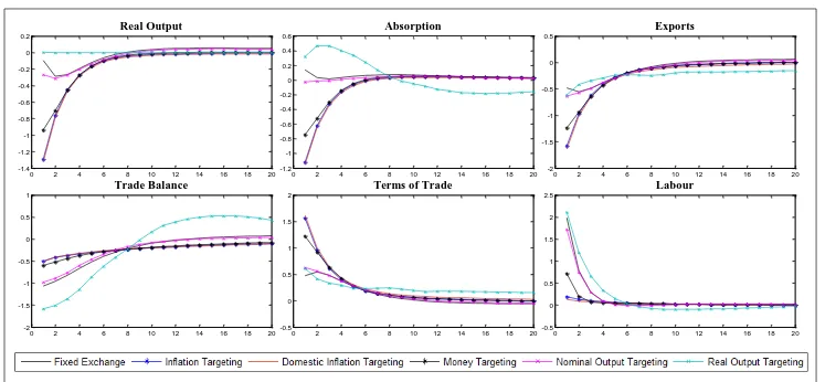
2.3.1 Domestic productivity shock………. 2.3.2 Foreign interest rate shock………. 2.3.3 Foreign output shock………. 2.3.4 Evaluation of monetary policy rules……….. 2.3.5 Robustness analysis………... 2.4 Conclusion..……….... Appendix 1.A Graphical representation of the model………..

6 6 13 13 15 20 21 21 22 23 27 27 32 33 36 48 48 50 3 EXTERNAL SHOCKS AND THE SRI LANKAN ECONOMY: A SVAR

APPROACH………... 3.1 Introduction……….... 3.2 Methodology………...

3.2.1 SVAR model framework………... 3.2.2 Block exogeneity assumption………

(10)

x

3.2.3 Non-recursive identification scheme………. 3.2.4 Data and estimation………...

58 60 3.3 Results………

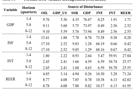
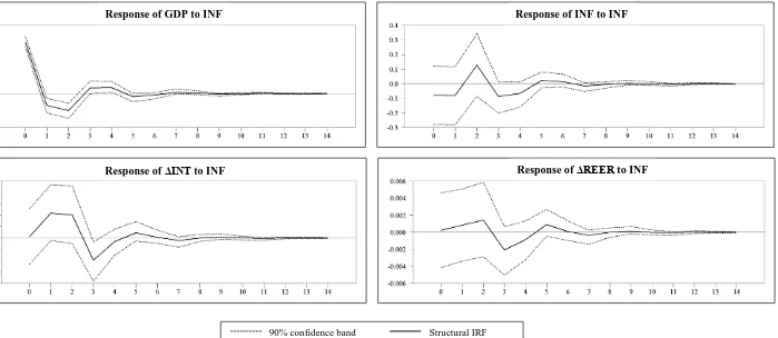
3.3.1 Impulse responses……….. 3.3.2 Forecast error variance decomposition……… 3.3.3 Historical decomposition………... 3.4 Alternative measure of foreign monetary policy……… 3.5 Robustness………..……… 3.6 Conclusion………..……… Appendix 3.A Unit root tests…..……….. Appendix 3.B Impulse responses of the EFFR model……… Appendix 3.C Historical decomposition of the EFFR model……… Appendix 3.D Domestic monetary policy shock under the Cholesky Identification………. Appendix 3.E Impulse responses of the SSR model……… Appendix 3.F Historical decomposition of the SSR model………

62 62 69 72 75 77 78 80 81 84 86 87 94 4 TERMS OF TRADE AND THE SRI LANKAN ECONOMY: A

SIGN-RESTRICTED VAR APPROACH……… 4.1 Introduction……….... 4.2 Methodology………...

4.2.1 Baseline VAR model ………... 4.2.2 From reduced-form VAR model to sign-restricted VAR….

4.2.3 Identification of shocks……….. 4.3 Results………...

4.3.1 Impulse responses……….. 4.3.2 Forecast error variance decomposition……….. 4.3.3 Historical decomposition………... 4.4 External shocks and trade………... 4.5 Robustness check……… 4.6 Conclusion……….. Appendix 4.A Data description and data sources………. Appendix 4.B Foreign and domestic data……… Appendix 4.C Unit root tests……… Appendix 4.D Impulse responses for robustness check………...

(11)

xi

5 CONCLUSION

5.1 Summary of findings and policy recommendations………... 5.2 Future research directions………...

150 150 152

(12)

xii

LIST OF FIGURES

FIGURE PAGE

2.1 External debt of Sri Lanka (2000-2014)………. 11 2.2 Quarter on quarter CPI inflation in Sri Lanka……… 11 2.3 Dynamic responses of real variables to a negative domestic

productivity shock………... 28

2.4 Dynamic responses of nominal and financial variables to a negative

domestic productivity shock……… 29

2.5 Dynamic responses of real variables to a contractionary foreign

interest rate shock……… 30

2.6 Dynamic responses of nominal and financial variables to a contractionary foreign interest rate shock……… 31 2.7 Dynamic responses of real variables to a negative foreign output

shock……… 34

2.8 Dynamic responses of nominal and financial variables to a negative

foreign output shock……… 35

2.A.1 DSGE model for Sri Lanka……….. 50

3.1 Foreign and domestic macroeconomic data (1996Q2 – 2014Q4)…... 61 3.2 Impulse responses to a domestic contractionary monetary policy

shock (EFFR model)……… 64

3.3 Impulse responses to a foreign contractionary monetary policy shock

(EFFR model)……… 65

3.4 Impulse responses to an oil price shock (EFFR model)……... 67 3.5 Impulse responses to a foreign output shock (EFFR model)………... 70 3.6 Historical decomposition of domestic output growth (EFFR model). 73 3.7 Historical decomposition of domestic inflation (EFFR model)... 74 3.8 Quarterly US shadow short rate………... 76 3.B.1 Impulse responses to a domestic output growth shock (EFFR

model)……….. 81

3.B.2 Impulse responses to a domestic inflation shock (EFFR model)…… 82 3.B.3 Impulse responses to an exchange rate shock (EFFR model)………. 83 3.C.1 Historical decomposition of change in the domestic interest rate

(13)

xiii

xii

i

3.C.2 Historical decomposition of change in the real effective exchange

rate (EFFR model)………. 85

3.D.1 Impulse responses to a contractionary monetary policy shock with the

Cholesky identification……….. 86

3.E.1 Impulse responses to an oil inflation shock (SSR model)…... 87 3.E.2 Impulse responses to a foreign output growth shock (SSR

model)……….. 88

3.E.3 Impulse responses to a foreign contractionary monetary policy shock

(SSR model)……….. 89

3.E.4 Impulse responses to a domestic output growth shock (SSR model).. 90 3.E.5 Impulse responses to a domestic inflation shock (SSR model)……... 91 3.E.6 Impulse responses to domestic contractionary monetary policy shock

(SSR model)……….. 92

3.E.7 Impulse responses to an exchange rate shock (SSR model)………… 93 3.F.1 Historical decomposition of domestic output (SRR model)………… 94 3.F.2 Historical decomposition of domestic inflation (SRR model)……… 95 3.F.3 Historical decomposition of change in the domestic interest rate

(SRR model)……… 96

3.F.4 Historical decomposition of change in the real effective exchange

rate (SRR model)……… 97

4.1 Selected macroeconomic variables of Sri Lanka………. 100 4.2 Impulse responses of foreign variables to a positive world demand

shock…... 110 4.3 Impulse responses of foreign variables to a negative world supply

shock……… 111

4.4 Impulse responses of foreign variables to a positive globalization

shock……… 112

4.5 Impulse responses of domestic variables to a positive world demand

shock……… 115

4.6 Impulse responses of domestic variables to a negative world supply

shock……… 116

4.7 Impulse responses of domestic variables to a positive globalization

shock……….. 117

(14)

xiv

4.9 Impulse responses of the trade related variables to a positive world

demand shock ………. 124

4.10 Impulse responses of the trade related variables to a negative world supply shock……….... 125

4.11 Impulse responses of the trade related variables to a positive globalization shock……….. 126

4.12 Historical decomposition of the trade balance, exports and imports. 128 4.B.1 Export prices……….. . 135

4.B.2 Import prices……….. . 135

4.B.3 Foreign output……….. 135

4.B.4 Domestic output……….. 135

4.B.5 Domestic prices………... 135

4.B.6 Domestic interest rate..……….... 135

4.B.7 Real effective exchange rate……… 136

4.B.8 Trade balance………... 136

4.B.9 Exports………. 136

4.B.10 Imports………. 136

4.D.1 Impulse responses to a positive world demand shock - VAR (1)….. 138

4.D.2 Impulse responses for to a negative world supply shock - VAR (1).. 139

4.D.3 Impulse responses to a positive globalization shock - VAR (1)…… 140

(15)

xv

LIST OF TABLES

TABLE PAGE

2.1 Calibration of the model………. 25

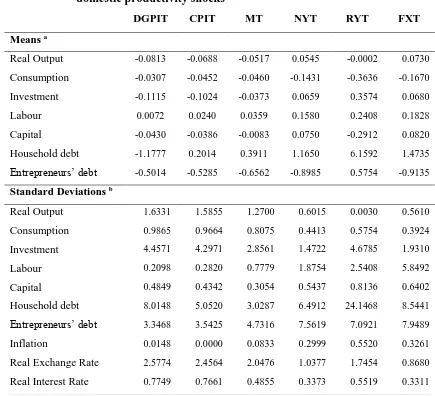
2.2 Mean and standard deviation of the domestic variables under domestic productivity shocks……….. 38

2.3 Mean and standard deviation of the domestic variables under foreign interest rate shocks……… 39

2.4 Mean and standard deviation of the domestic variables under negative foreign output shocks……… 40

2.5 Unconditional welfare measures……….. 45

2.6 Conditional welfare measures……….. 46

3.1 Lag structure of the model………... 58

3.2 Forecast error variance decomposition (EFFR model)………... 71

3.3 Forecast error variance decomposition (SSR model)………. 77

3.A.1 Summary of unit root tests………... 80

4.1 Lag structure of the model………... 105

4.2 Sign-restrictions………... 108

4.3 Forecast error variance decomposition……… 119

(16)

1

CHAPTER 1

INTRODUCTION

1.1 Motivation

During the past few decades, economic shocks originating from unbalanced demand, unanticipated supply-side disturbances and financial market failures have rippled across the global economy numerous times. The ramifications of the global financial crisis in 2007-2009 have been a stark reminder of the economic interdependence of both developed and developing countries. Consequently, policy-makers around the world are becoming increasingly concerned about the uncertain impact of such foreign shocks on their domestic economies. These recent events also call for a thorough examination of appropriate domestic policy responses that strengthen the economic resilience towards possible external shocks.

(17)

2

Sri Lanka’s trade liberalization process was initiated in 1977, ahead of its neighbours, as a response to the dismal economic outcomes of protectionist trade policies. Although Sri Lanka’s trade reforms progressed at a ‘mixed pace’, it remained committed to integrating with global markets during past four decades. Sri Lanka’s international trade was boosted substantially due to the trade reforms but the trade balance continued to be a deficit over the years. Liberalization of both the current and capital account of Sri Lanka also commenced parallel to the trade liberalization process. Although Sri Lanka’s current account was fully liberalized by 1994, policy-makers of Sri Lanka have been more cautious and reluctant in fully liberalizing the capital account. This is not surprising given the country’s perpetual fiscal imbalances and the large external debt stock.

The Central Bank of Sri Lanka adopted a floating exchange rate regime in 2001, but by and large the exchange rate has been tightly managed over the years to avoid potential difficulties in foreign debt servicing due to excessive currency depreciation. Further, the Central Bank of Sri Lanka still follows a monetary aggregate targeting regime. However, Anand et al. (2011) show that the Central Bank gives higher weight to the domestic output growth and lower weight to domestic inflation, which is a sub-optimal monetary policy rule under domestic shocks.

(18)

3

1.2 Structure of the thesis

This dissertation consists of five chapters. Chapters 2 to 4 present three self-contained essays. The last chapter concludes, highlighting the policy implications and future research directions.

Chapter 2, titled ‘External shocks and monetary policy in Sri Lanka’ investigates, the role of monetary policy in insulating the domestic economy from both domestic and external shocks. This chapter uses a small open economy Dynamic Stochastic General Equilibrium (DSGE) model with financial frictions, delayed exchange rate pass-through and nominal price rigidities to assess the welfare implications of alternative monetary policy rules. This study compares six monetary policy rules, namely, consumer price inflation targeting, domestic goods inflation targeting, monetary aggregate targeting, nominal income targeting, real income targeting and fixed exchange rate targeting rules. The welfare losses under domestic productivity shocks, foreign interest rate shocks and foreign output shocks are estimated for the six alternative policy rules. The model is calibrated to represent the Sri Lankan economy.

The alternative monetary policy rules are compared and ranked based on the conditional and unconditional welfare of the households, taking second-order approximation of the full set of model equations. Further, the welfare losses under alternative monetary policy rules are decomposed into two parts: the welfare effects of uncertainty on the variance and the welfare effects of uncertainty on the means of the macro-variables. As the effect of uncertainty on the means of the macro-variables have a significant welfare implication, this study highlights the need for taking the second-order approximation of the full set of model equations in welfare analysis.

(19)

4

the effect of US monetary policy using two measures: the Effective Federal Funds Rate (EFFR) and the US Shadow Short Rate (SSR). While the EFFR is the policy rate, the SSR captures the overall monetary policy stance of the Federal Reserves of the US including the unconventional monetary policy measures such as quantitative easing. To the best of my knowledge, this is the first paper that investigates the effect of overall monetary policy stance of the US on the Sri Lankan economy using a SVAR framework.

Chapter 4, titled ‘Terms of trade and the Sri Lankan economy: a sign-restricted VAR approach’, investigates the effect on the Sri Lankan economy of external shocks that cause terms of trade fluctuations. The traditional approach of modelling the terms of trade shocks in the SVAR literature is to incorporate the terms of trade variable directly into the model with the rest of the foreign and domestic variables. However, in the recent literature, such as that contributed by Jääskelä and Smith (2013) and Karagedikli and Price (2012), it has been argued that the fluctuations in the terms of trade are driven by

different underlying external shocks. If these underlying shocks are not specified in the

VAR model, the reverse causality coming from other foreign variables on the terms of

trade variable may not be captured properly. Further, they argue that the effect of terms

of trade shocks on the domestic macroeconomy depends on the characteristics of external

shocks underlying the terms of trade fluctuations.

Following the approach of Jääskelä and Smith (2013) and Karagedikli and Price (2012),

this paper uses a sign-restricted VAR model to investigate the effect on the Sri Lankan

macroeconomic variables from the external shocks that cause movements in terms of

trade. The terms of trade fluctuations for the Sri Lankan economy are assumed to be

driven by world demand shocks, world supply shocks and globalization shocks. To the

best of my knowledge, this is the first research paper that applies the sign-restricted VAR

methodology for the Sri Lankan economy. Further, the model uses a newly constructed

foreign output variable, which represents the output of 13 major trading partners of Sri

Lanka. Extending the model of Jääskelä and Smith (2013) and Karagedikli and Price

(2012), this essay also investigates the effect of terms of trade fluctuations on the exports,

imports and the trade balance of Sri Lanka. The findings of this chapter show that the

(20)

5

insulating the domestic economy compared to the free float exchange rate policy used in Australia and New Zealand.

(21)

6

CHAPTER 2

EXTERNAL SHOCKS AND MONETARY POLICY IN SRI LANKA

2.1 Introduction

With increasing globalization, external shocks have become an important source of macroeconomic fluctuations in developing and emerging economies. This is evident from developing countries’ experience in the past few decades, especially during the periods of oil and commodity price escalation and the Asian and global financial crises. Unanticipated macroeconomic fluctuations caused by external shocks can have a considerable welfare effect on developing countries. Within this milieu, the monetary authority of a small open economy needs to consider the welfare effect of external shocks when selecting an appropriate monetary policy regime for the country. Following the example of many developed countries, should the central banks of small open economies allow the exchange rates to float and target inflation? What measure of inflation would best insulate the economy from external shocks? Is an inflation targeting regime harmful for the welfare of economies burdened with foreign currency denominated debt? Is a monetary policy regime geared to target domestic output more welfare-superior than an inflation targeting regime for developing economies? These are some of the questions that many economists still debate (Monacelli, 2005, Devereux et al., 2006, Elekdag & Tchakarov, 2007, Schmitt-Grohe & Uribe, 2004, McKibbin & Singh 2003, Alba et al. 2011, Summer 2011).

(22)

7

Many theoretical studies have shown the welfare-superiority of inflation targeting and Taylor-type rules over other monetary policy rules. Using a small open economy DSGE model with staggered-prices, complete exchange rate pass-through and complete financial markets, Gali and Monacelli (2005) show that the domestic inflation-based Taylor rule performs better than the Consumer Price Index (CPI)-based Taylor rule and the exchange rate peg in terms of minimizing social welfare losses. Alba et al. (2011) use a similar model and assert that the Taylor-rule is appropriate for countries with very low import-to-GDP ratio as it simultaneously stabilizes the output and inflation. In contrast, the CPI-based inflation targeting rule is suitable for countries with high import dependency. If the import dependency is very high (i.e., the imports-to-GDP ratio is one or more), exchange rate targeting and CPI-based inflation targeting provide equally better results.

Moving forward, Devereux et al. (2006) assume incomplete exchange rate pass-through and external borrowing constraints in addition to the staggered price setting behaviour in a small open economy. They assert that external financing constraints do not have a significant effect on the ranking of the monetary policy rules, but such constraints magnify the responses of macroeconomic variables to the external shocks. Conversely, the degree of exchange rate pass-through is an important factor affecting the ranking of monetary policy rules. Their findings affirm the results of Gali and Monacelli (2005) and posit that domestic inflation targeting is appropriate for economies with high exchange rate pass-through. But in economies with low-exchange rate pass-through, the prices of both domestic and imported goods adjust slowly, making CPI-based inflation targeting more effective.

(23)

8

dollarization if the debt-to-GDP ratio is low. However, a fixed exchange rate regime can be more welfare-superior than a floating exchange rate regime when the debt-to-GDP ratio exceeds 79 per cent. They claim that a fixed exchange rate regime can outperform the floating exchange rate regime particularly when the shocks are emanating from external sources. Kolasa and Lombardo (2011) also argue that pure inflation targeting can be sub-optimal when the economy has foreign-currency-denominated debt. Moreover, Eichengreen (2002) concludes that conventional inflation targeting will be viable as long as the shocks and the corresponding exchange rate movements are small, and the desire to intervene and stabilize the exchange rate will dominate when they grow large. Further, De Paoli (2009) asserts that for sufficiently large values of inter-temporal elasticity of substitution, the exchange rate targeting rule will outperform the domestic inflation targeting rule in terms of welfare.

On the other hand, some economists favour the concept of nominal income targeting policies (Hall & Mankew 1993, McCallum & Nelson 1999) over inflation targeting. Although many developed and developing countries embraced the inflation targeting regime during the past two decades, the recent global economic crisis has raised questions regarding the welfare-superiority of inflation targeting regimes. The central banks that were adopting the inflation targeting rules were not able to prevent economic downturn as they were solely focusing on inflation management. Hence, the concept of nominal income targeting, which was introduced in 1980s, is now receiving revived interest (Summer 2011). McKibbin and Singh (2003) use the MSG2 model, which is a fully specified dynamic inter-temporal general equilibrium model, to investigate the effective monetary policy regimes for the Indian economy. This study shows that monetary aggregate and nominal output targeting rules are performing better than the inflation targeting rule in terms of stabilizing real output. Hence, nominal income targeting could be an appropriate monetary policy rule for countries that undergo significant structural adjustment. In contrast, Schmitt-Grohe and Uribe (2007) posit that interest rate rules that respond to real output lead to substantial welfare losses.

(24)

9

has a higher weight on the inflation gap and a lower weight on the output gap than the weights in the empirically estimated model for Sri Lanka. They also assert that an inflation targeting regime would have a more superior performance than would a monetary targeting regime in terms of stabilizing the macro-economic variables. However, Anand et al. (2011) have considered only domestic shocks and have not taken in to account any external shocks.

The Sri Lankan economy is particularly vulnerable to external shocks for a number of reasons. Sri Lanka’s export sector heavily relies on a few products such as garments and textiles, tea, rubber and coconut. Most Sri Lankan exports, especially the agricultural commodities, are low value-added, non-differentiated products. Consequently, Sri Lanka does not have significant market power in relation to its exports and the country’s terms of trade is highly volatile, depending on global market prices. Further, lack of diversification of export destination also intensifies the country’s vulnerability to external shocks. During the past decade, the United States and European Union has accounted for more than half of Sri Lankan exports annually. Hence, a decline in demand in advanced economies has a significant impact on Sri Lanka’s export sector as observed during the recent global financial crisis. Further, Sri Lanka is heavily dependent on petroleum imports for energy. For example, 36.9 per cent of Sri Lanka’s primary energy requirement was met by petroleum products in 2013 (Sri Lanka Sustainable Energy Authority, 2013). Moreover, 25.4 per cent of electricity, which is the main secondary energy source in Sri Lanka, was generated by thermal power using petroleum products during the same year (despite this being a year with a very good rainfall and the highest recorded hydropower generation in the history of Sri Lanka). During 2013, petroleum products accounted for 23 per cent of Sri Lanka’s import costs (Central Bank of Sri Lanka, 2013). Hence, price fluctuations in global energy markets tend to have an impact on the inflation and output of Sri Lanka.

(25)

10

stock in the economy, Sri Lanka is vulnerable to a balance of payments crisis in the event of a sudden stop or reversal of foreign capital flows.

Monetary policy in Sri Lanka

One of the core objectives of the Central Bank of Sri Lanka (CBSL) is economic and price stability. Although many countries have adopted inflation targeting regimes, the CBSL still adopts a monetary aggregate targeting system to implement its monetary policies. The CBSL uses Reserve Money as the operational target and Broad Money (M2b) as the intermediate target to achieve its price stability objective. The main

instruments used by the CBSL for its monetary management are (a) policy rates (i.e., Repurchase and Reverse Repurchase Rates) and open market operations (b) Statutory Reserve Ratio (SRR). Nevertheless, the reliance on SRR as a day-to-day monetary management tool has been gradually reduced by the CBSL to enhancing market orientation of monetary policy and to reduce the implicit cost of funds borne by the commercial banks due to SRR.

As depicted in Figure 2.2, the CBSL has been able to manage the country’s inflation at a single digit level since 2009, which is a great achievement compared to the past. Although the country has never gone through any hyper-inflation periods, inflation rates in Sri Lanka have been relatively high until 2009. Hence, multilateral donor organizations such as the International Monetary Fund (IMF) have suggested that the CBSL adopt an inflation targeting framework to better manage domestic inflation and continue with the current low inflation rates (Anand et al. 2011).

(26)

11

[image:26.842.60.762.142.356.2]

Figure 2.1 External debt of Sri Lanka (2000-2014) Figure 2.2 Quarter on quarter CPI inflation in Sri Lanka

Source: Annual Report of Central Bank of Sri Lanka, 2014 Source: International Financial Statistics Database

0 10 20 30 40 50 60 70 80 90 100 0 5,000 10,000 15,000 20,000 25,000 30,000 35,000 40,000 45,000 50,000 % of G D P U S$ mi ll ion

Total External Debt External Debt as a Percentage of GDP

(27)

12

market by buying/selling foreign currency at or near market rates in order to prevent any substantial exchange rate movements and to build-up reserves. For countries such as Sri Lanka where financial markets are thin and not well-developed, foreign currency market interventions are necessary to manage the excessive volatility of exchange rates. However, as Anand et al. (2011) point out, the real objective of the CBSL in its foreign exchange market intervention is ambiguous due to a relative lack of transparency of the CBSL. For example, it is difficult for the markets to assess whether CBSL is focusing on excess volatility or on the level of the exchange rate because what is considered as excess volatility is usually not well defined, while the pattern of intervention is not always consistent with volatility developments (Anand et al. 2011). Therefore, on many occasions the IMF has advised the CBSL to limit its foreign exchange market intervention and allow the currency to free float.

Currently, there is a debate over whether Sri Lanka can move in to inflation targeting under existing macroeconomic conditions. According to Perera (2010), the statistical relationship between the operating and final targets of an inflation targeting regime is not sufficiently strong, significant and persistent for the Sri Lankan economy. However, Perera (2010) also claims that such linkages are beginning to emerge in the Sri Lankan economy with economic and financial sector developments. However, the conflict of interest of the CBSL will be an obstacle for Sri Lanka to move in to inflation targeting. At present, the Employees’ Provident Fund, which is the biggest domestic lender to the government, and the public debt management department are under the purview of the CBSL. In that context, CBSL may not be able to credibly commit to an inflation targeting system. Nevertheless, the scope of this essay does not entail the investigation of pre-requisites for inflation targeting. Instead, this essay focus on assessing the welfare implications of different monetary policy rules under shocks emanating from external sources.

(28)

13

rules are next in order in terms of welfare. Strict exchange rate targeting is worst in welfare performance under both types of foreign shocks.

2.2 Model

The model consists of households, final goods producing firms, intermediate capital goods producing firms, entrepreneurs, importers, monetary authority and a foreign economy. The model is graphically presented in Appendix 1.A.

2.2.1 Consumers

The small open economy is populated by a continuum of infinitely lived, utility-maximizing households. The inter-temporal utility function of the households depends positively on consumption (Ct) and real money holdings (Mt/Pt) and negatively on the labour supply (Ht). The utility of households can be defined as below:

𝑈 = 𝐸0∑ β𝑡( 𝐶𝑡1−𝜎

1−𝜎 − 𝐻_𝑡1+𝜂

1+𝜂 + (𝑀𝑡

𝑃𝑡) 1−𝜉

1−𝜉 ) ∞

𝑡=0 (2.1)

where 𝛽∊(0,1) is the discount factor, σ, 𝜂 and 𝜉 are the inverse of the elasticity of inter-temporal substitution for consumption, labour and real money balance. Pt is consumer price index. Households consume a basket of differentiated goods comprising of domestic and imported goods. Composite consumption basket is a CES function defined as follows:

𝐶_𝑡 = [(𝑎)𝜃1 𝐶

𝐻,𝑡 𝜃−1

𝜃 ⁄

+ (1 − 𝑎)1𝜃 𝐶

𝐹,𝑡 𝜃−1 𝜃 ⁄ ] 𝜃 𝜃−1 ⁄ (2.2)

where CH and CFdenote the domestic and imported goods, respectively. θ is the elasticity of substitution between domestic and imported goods and θ > 0. The share of domestic goods in the household consumption basket is a and a ∊ (0,1). CH and CF can be defined as

𝐶𝐻,𝑡 = [∫ 𝐶𝐻,𝑡 1

0 (𝑗)

1−𝜆_𝑑𝑗]1/1−𝜆 _(2.3)

and

𝐶𝐹,𝑡 = [∫ 𝐶𝐹,𝑡 1

0 (𝑗)

1−𝜆_𝑑𝑗]1/1−𝜆 _(2.4)

𝐶_𝐻(𝑗) and 𝐶_𝐹(𝑗) stand for the consumption of variety j of domestic and imported goods,

(29)

14

consumer price index, Pt, associated with the composite consumption basket in (2.2) is defined as follows:

𝑃𝑡 = [(𝑎)

1 𝜃 𝑃

𝐻,𝑡 𝜃−1

𝜃 ⁄

+ (1 − 𝑎) 1 𝜃 𝑃

𝐹,𝑡 𝜃−1 𝜃 ⁄ ] 𝜃 𝜃−1 ⁄ (2.5) where, 𝑃𝐻(𝑗) and 𝑃𝐹(𝑗) are the prices of individual domestic and imported goods j,

respectively, in terms of domestic currency. 𝑃_𝐻 and 𝑃_𝐹 can be expressed as 𝑃𝐻,𝑡 = [∫ 𝑃𝐻,𝑡

1

0 (𝑗)

1−𝜆_𝑑𝑗]1/1−𝜆 _(2.6)

and

𝑃_𝐹,𝑡 = [∫ 𝑃𝐹,𝑡 1

0 (𝑗)

1−𝜆_𝑑𝑗]1/1−𝜆 _(2.7)

The optimal allocation of expenditure between domestic and imported goods can be expressed as follows:

𝑚𝑖𝑛𝐶𝐻,𝐶𝐹𝑃𝑡𝐶𝑡 = 𝑃𝐻𝐶𝐻+ 𝑃𝐹𝐶𝐹 s.t

𝐶_𝑡 = [(1 − 𝑎)1𝜃 𝐶

𝐻 𝜃−1

𝜃 ⁄

+ (𝑎)1𝜃 𝐶

𝐹 𝜃−1 𝜃 ⁄ ] 𝜃 𝜃−1 ⁄ (2.8) This optimization problem yields the following demand functions for domestic and imported goods:

𝐶_𝐻,𝑡 = (𝑎) (𝑃𝐻,𝑡

𝑃𝑡 )

−𝜃

𝐶_𝑡 (2.9)

𝐶_𝐹,𝑡 = (1 − 𝑎) (𝑃𝐹,𝑡

𝑃𝑡 )

−𝜃

𝐶_𝑡 (2.10)

The households own the monopolistic firms in the economy and also provide labour to the firms. Hence, households receive income in the form of wage (𝑊_𝑡) and profits (П_𝑡). The household budget constraint in period t can be written as follows:

𝑃_𝑡𝐶_𝑡= 𝑊_𝑡𝐻_𝑡+ (1 + 𝑟_𝑡)𝐵_𝑡− 𝐵_𝑡+1+ 𝑀_𝑡− 𝑀_𝑡−1+ 𝑆_𝑡𝐷_𝑡+1

− (1 + 𝑟_𝑡∗_)𝛹

𝐷,𝑡𝑆𝑡𝐷𝑡+ П𝑡 (2.11)

where 𝐵_𝑡and 𝐷_𝑡 are the nominal stock of domestic-currency denominated bonds and foreign-currency-denominated debt maturing in period t.

The domestic-currency bonds earns a nominal interest rate of 𝑟𝑡. In period t, households

have to spend (1 + 𝑟𝑡∗)𝛹𝐷,𝑡 amount as the interest payments on foreign debt. 𝑟𝑡∗ is the

foreign nominal interest rate. The country risk premium denoted by 𝛹𝐷,𝑡 depends on the

(30)

15

a modified version of the country risk premium used by Adolfson et al. (2007). Accordingly,

𝛹_𝐷,𝑡 = 𝑒𝑥𝑝[𝜓_𝐷(𝑇𝐷_𝑡− 𝑇𝐷)] (2.12) where 𝑇𝐷_𝑡 is the aggregate foreign debt level in the economy, 𝑇𝐷 is the steady state foreign debt level and 𝜓𝐷 is the elasticity of the country risk-premium with respect to the

aggregate foreign debt level. Further,

𝑇𝐷𝑡= 𝑆𝑡(𝐷𝑡+ 𝐷𝐸,𝑡)/𝑃𝑡 (2.13)

where 𝐷𝐸,𝑡is the foreign debt stock held by the entrepreneurs in the economy.

The household problem can be written as

max_𝐶_𝑡_,𝐻_𝑡_,𝐵_𝑡_,𝑀_𝑡,_𝐷_𝑡 𝑈 = 𝐸₀∑ β𝑡(𝐶𝑡1−𝜎

1−𝜎 − 𝐻_𝑡1+𝜂

1+𝜂 + (𝑀𝑡

𝑃𝑡) 1−𝜉

1−𝜉 ) ∞

𝑡=0 s.t

𝑃𝑡𝐶𝑡 = 𝑊𝑡𝐻𝑡+ (1 + 𝑟𝑡)𝐵𝑡− 𝐵𝑡+1+ 𝑀𝑡− 𝑀𝑡−1+ 𝑆𝑡𝐷𝑡+1

−(1 + 𝑟𝑡∗)𝛹𝐷,𝑡𝑆𝑡𝐷𝑡+ П𝑡 (2.14)

The household optimum can be characterized by the following conditions: 𝛽_𝑡 𝐸 ( 𝐶𝑡𝜎𝑃𝑡

𝐶_𝑡+1𝜎 𝑃𝑡+1) =

1

1+𝑟𝑡+1 (2.15)

𝛽𝑡 𝐸 ( 𝐶𝑡𝜎𝑃𝑡

𝐶𝑡+1𝜎 𝑃𝑡+1) =

1 𝛹𝐷,𝑡+1(1+𝑟𝑡+1∗ )

(2.16) 𝑊𝑡 = 𝑃𝑡𝐻𝑡

𝜂

𝐶_𝑡𝜎 (2.17)

(𝑀𝑡

𝑃𝑡)

−𝜉

= 𝐶−𝜎_{(1 −} 1

(1+𝑟𝑡+1)) (2.18)

Equations (2.15) and (2.16) represent the Euler equations for consumption in relation to domestic and foreign interest rates. The supply of labour is given by equation (2.17) while the money demand is described by equation (2.18).

2.2.2 Firms

The economy comprises of four types of firms, namely, final goods producing firms, intermediate capital goods producers, entrepreneurs and importers.

Final goods producing firms

(31)

16

Therefore, the effective labour of production firm i can be defined as 𝐿_𝑡(𝑖) = 𝐻_𝑡(𝑖)𝛺_𝐻

𝑡𝑒(𝑖)1−𝛺 (2.19)

where 𝐿𝑡(𝑖) is the effective labour of the firm, 𝐻𝑡(𝑖) is the labour employed from

households and 𝐻_𝑡𝑒_(𝑖)_{is the employment of entrepreneurial labour.}

The production technology function of production firm i can be expressed as

𝑌_𝑡(𝑖) = 𝐴𝑡𝐾𝑡(𝑖)𝛼𝐿𝑡(𝑖)1−𝛼 (2.20)

where 𝐴𝑡is the technology parameter, 𝑌𝑡(𝑖) is the output and 𝐾𝑡(𝑖) is the capital of the

firm 𝑖. 𝛼∊ (0,1) is capital income share. In this study 𝐴_𝑡 follows an AR(1) process. Then 𝐴𝑡 = 𝜁𝐴 𝐴𝑡−1 + (1 − 𝜁𝐴) A + 𝜀𝐴,𝑡 (2.21)

The cost minimization problem of the final goods-producing firms can be given as 𝑀𝑖𝑛_𝐾_𝑡_,𝐻_𝑡_,𝐻_𝑡𝑒 𝐶 = 𝑅_𝑡𝐾_𝑡+ 𝑊_𝑡𝐻_𝑡+ 𝑊_𝑡𝑒𝐻_𝑡𝑒 s.t.

𝑌𝑡 = 𝐴𝑡𝐾𝑡𝛼(𝐻𝑡𝛺𝐻𝑡𝑒1−𝛺) 1−𝛼

(2.22)

where 𝑊_𝑡𝑒 is the nominal wage of entrepreneurs and 𝑅𝑡 is the nominal rental rate of

capital.

The final goods producing firms’ optimum conditions can be expressed as follows: 𝑅_𝑡= 𝑛𝑚𝑐_𝑡(𝛼)𝑌𝑡

𝐾𝑡 (2.23)

𝑊𝑡 = 𝑛𝑚𝑐𝑡(1 − 𝛼)𝛺 𝑌𝑡

𝐻𝑡 (2.24)

𝑊_𝑡𝑒 = 𝑛𝑚𝑐_𝑡(1 − 𝛼)(1 − 𝛺)𝑌𝑡

𝐻_𝑡𝑒 (2.25)

where 𝑛𝑚𝑐_𝑡is the nominal marginal cost.

Following Rotemberg (1982), it is assumed that the final goods-producing firms set their prices as monopolistic competitors and each firm has to incur a small direct cost in the event of price adjustment. Consequently, firms adjust their prices gradually rather than instantaneously in response to a shock to the marginal cost or the demand. The final goods producing firms maximize their expected profits stream using the following discount factor:

𝛤_𝑡+1 = ( 𝑃𝑡𝐶𝑡𝜎

𝑃𝑡+1𝐶𝑡+1𝜎

) 𝛽 (2.26)

(32)

17

Accordingly, production firm (i) maximizes the following objective function: 𝐸0∑∞𝑡=0𝛤𝑡{𝑃𝐻,𝑡(𝑖)𝑌𝑡(𝑖) − 𝑛𝑚𝑐𝑡 𝑌𝑡(𝑖) − 𝑃𝑡

𝜓_𝑃𝐻 2 [

𝑃𝐻,𝑡(𝑖)− 𝑃𝐻,𝑡−1(𝑖)

𝑃𝐻,𝑡(𝑖) ]

2

} s.t.

𝑌_𝑡(𝑖) = (𝑃𝐻,𝑡(𝑖)

𝑃𝐻,𝑡 )

−𝜆

𝑌_𝑡 (2.27)

where 𝑃_𝐻,𝑡(𝑖) and 𝑌_𝑡(𝑖) are the price and the demand for the product of firm (i). Further, 𝑃𝑡

𝜓_𝑃𝐻 2 [

2

represents the price adjustment cost.

Since all the firms in the economy are identical, the optimal price setting equation can be expressed as

𝑃_𝐻,𝑡 = 𝜆

𝜆−1𝑛𝑚𝑐𝑡− 𝜓_𝑃𝐻 𝜆−1

𝑃𝑡

𝑌𝑡

𝑃𝐻,𝑡

𝑃𝐻,𝑡−1 (

𝑃𝐻,𝑡

𝑃𝐻,𝑡−1− 1) +

𝜓_𝑃𝐻 𝜆−1 𝐸𝑡[

𝛤𝑡+1

𝛤𝑡

𝑃𝑡+1

𝑌𝑡

𝑃𝐻,𝑡+1

𝑃𝐻,𝑡 (

𝑃𝐻,𝑡+1

𝑃𝐻,𝑡 − 1)] (2.28) when 𝜓_𝑃_𝐻 = 0, the firms’ price is equal to a mark-up over nominal marginal cost.

Intermediate capital goods producers

The role of intermediate capital goods producers is to build new intermediate capital using existing depreciated capital and new investments within a competitive market. The capital producers buy a fraction of the domestic final goods and imported goods to produce the investment goods 𝐼_𝑡. The mix of domestic goods and imported goods in the capital producers’ purchases is similar to the household consumption basket. Thus the nominal price of unit of investment is equal to 𝑃𝑡. The composite investment good

comprised of domestic and imported goods can be expressed as 𝐼_𝑡 = [(𝑎)1𝜃 𝐼

𝐻,𝑡 𝜃−1

𝜃 ⁄

+ (1 − 𝑎)1𝜃 𝐼

𝐹,𝑡 𝜃−1 𝜃 ⁄ ] 𝜃 𝜃−1 ⁄ (2.29) where 𝐼𝐻,𝑡 and 𝐼𝐹,𝑡 are the domestic goods and foreign goods used in private capital

production, respectively. Accordingly, 𝐼_𝐻,𝑡 = (𝑎) (𝑃𝐻,𝑡

𝑃𝑡 )

−𝜃

𝐼_𝑡 (2.30)

𝐼_𝐹,𝑡 = (1 − 𝑎) (𝑃𝐹,𝑡

𝑃𝑡 )

−𝜃

𝐼_𝑡 (2.31)

The capital producers face a nominal quadratic adjustment cost in the following form:

𝜓𝐼

2 ( 𝐼𝑡

𝐾𝑡− 𝛿)

2

(33)

18

where 𝜓_𝐼is the degree of capital adjustment cost and 𝛿 is the depreciation rate. Therefore, the production technology of intermediate capital goods producers can be represented as

≡ (𝐼_𝑡, 𝐾_𝑡) = [𝐼𝑡

𝐾𝑡−

𝜓𝐼

2 ( 𝐼𝑡

𝐾𝑡− 𝛿)

2

] 𝐾_𝑡 (2.32)

Then the evolvement of capital in the economy can be expressed as 𝐾_𝑡+1 = [𝐼𝑡

𝐾𝑡−

𝜓𝐼

2 ( 𝐼𝑡

𝐾𝑡− 𝛿)

2

] 𝐾_𝑡+ (1 − 𝛿)𝐾_𝑡 (2.33)

The intermediate capital producers sell their intermediate capital product 𝐾_𝑡+1 to entrepreneurs at the price of 𝑄_𝑡. Then, the maximization problem of the capital producers can be written as follows:

𝑀𝑎𝑥𝐼𝑡 𝑃𝑟𝑜𝑓𝑖𝑡 = 𝑄𝑡([

𝐼𝑡

𝐾𝑡−

𝜓𝐼

2 ( 𝐼𝑡

𝐾𝑡− 𝛿)

2

] 𝐾𝑡+ (1 − 𝛿)𝐾𝑡)

− 𝑃_𝑡𝐼_𝑡− 𝑅_𝐾𝑈𝐾 (2.34)

where 𝑅_𝐾𝑈is the nominal rental rate paid by the intermediate capital goods producing firms to entrepreneurs who supply the capital. The aforementioned optimization problem yields

𝑄𝑡=

𝑃𝑡

1− 𝜓𝐼(_𝐾𝑡𝐼𝑡− 𝛿)

(2.35)

Entrepreneurs

Entrepreneurs supply capital to both final goods and intermediate capital producing firms. They also supply entrepreneurial labour to the final goods producing firms. In addition, entrepreneurs purchase intermediate capital goods.

(34)

19

If 𝑄_𝑡 and 𝑁_𝑡 are the price of capital and entrepreneurs’ net worth, respectively, balance sheet of the entrepreneurs can be expressed as follows:

𝑁𝑡+1= 𝑄𝑡𝐾𝑡+1− 𝑆𝑡𝐷𝐸,𝑡+1 (2.36)

where 𝑆𝑡 is the current period nominal exchange rate and 𝐷𝐸,𝑡denotes the entrepreneurs’

foreign debt. Equation (2.36) indicates that entrepreneurs’ net worth is the difference between their assets and liabilities. It also shows that unanticipated depreciation of the exchange rate worsens the net worth of the entrepreneurs.

The external-financing-premium of the entrepreneurs depends on the ratio of the internal and external financing:

𝛷_𝑡+1= (𝑄𝑡𝐾𝑡+1

𝑁𝑡+1 )

𝛾

(2.37) where γ is the elasticity of external-financing-premium with respect to leverage ratio. It is assumed that entrepreneurs are risk-neutral and would chose 𝐾_𝑡+1 and 𝐷_𝐸,𝑡+1in such a way to maximize their profits. The optimal financial contract between borrower and foreign lender ensures the expected marginal return on capital is equal to the expected marginal cost of external financing at t+1 period.

The expected marginal cost of the external borrowing is a function of the firm’s external borrowing premium, world interest rate, country-specific risk premium and unanticipated swings in the exchange rate:

𝐸_𝑡𝑅_𝐾,𝑡+1= 𝛷_𝑡+1(1 + 𝑟_𝑡+1∗ )𝛹_𝐷,𝑡+1𝐸_𝑡(𝑆𝑡+1

𝑆𝑡 ) (2.38)

Entrepreneurs’ expected return on capital has three components: the nominal rental on capital paid by the final goods producing firms, the nominal rental on capital paid by the intermediate capital goods producing firms and the value of undepreciated capital stock. Thus, entrepreneurs’ real return on capital after adjusting for asset price fluctuations can be expressed as follows:

𝑅𝐾,𝑡+1 = 𝑅𝑡+1

𝑄𝑡 + [1 − 𝛿 + 𝜓𝐼(

𝐼𝑡+1

𝐾𝑡+1− 𝛿)

𝐼𝑡+1

𝐾𝑡+1−

𝜓𝐼

2 ( 𝐼𝑡+1

𝐾𝑡+1− 𝛿)

2 ]𝑄𝑡+1

𝑄𝑡 (2.39)

(35)

20

unity. Hence, the entrepreneurs’ net worth at the end of period t, 𝑁_𝑡+1can be expressed as below:

𝑁_𝑡+1= 𝑣 [𝑅_𝐾,𝑡𝑄_𝑡−1𝐾_𝑡− (𝛷_𝑡(1 + 𝑟_𝑡∗_)𝛹 𝐷,𝑡(

𝑆𝑡

𝑆𝑡−1) (𝑄𝑡−1𝐾𝑡− 𝑁𝑡))] + 𝑊𝑡

𝑒_(2.40)

Entrepreneurs who do not survive for the next period will consume their net wealth. Therefore, the consumption of the entrepreneurs can be written as

𝐶_𝐸,𝑡 = {(1 − 𝑣) [𝑅_𝐾,𝑡𝑄_𝑡−1𝐾_𝑡− (𝛷_𝑡(1 + 𝑟_𝑡∗_{) 𝛹} 𝐷,𝑡(

𝑆𝑡

𝑆𝑡−1) (𝑄𝑡−1𝐾𝑡− 𝑁𝑡))]}

1 𝑃𝑡 (2.41)

Importers

Duma (2008) shows that the exchange rate pass-through in the Sri Lankan economy is low due to the existence of administered prices and government subsidies. Therefore, it is assumed that importers are operating in a monopolistically competitive market and there is incomplete exchange rate pass-through economy. Importers also have to incur a small direct cost of price adjustment. The maximization problem of importer (i) can be expressed as

𝐸0∑∞𝑡=0𝛤𝑡{𝑃𝐹,𝑡(𝑖)𝐼𝑀𝑡(𝑖) − 𝑆𝑡𝑃𝐹∗ 𝐼𝑀𝑡(𝑖) − 𝑃𝑡 𝜓_𝑃𝐹

2 [

𝑃𝐹,𝑡(𝑖)− 𝑃𝐹,𝑡−1(𝑖)

𝑃𝐹,𝑡(𝑖) ]

2

} s.t.

𝐼𝑀_𝑡(𝑖) = (𝑃𝐹,𝑡(𝑖)

𝑃𝐹,𝑡 )

−𝜆

𝐼𝑀_𝑡 (2.42) where 𝑃_𝐹,𝑡(𝑖) and 𝐼𝑀_𝑡(𝑖) are the price of imported goods in domestic currency and the demand for the imported product of importer (i). The term 𝑃𝑡

𝜓_𝑃𝐹 2 [

𝑃_𝐹,𝑡(𝑖) ] 2

denotes the price adjustment cost.

Since all the importing firms are identical, the optimal price setting equation can be written as

𝑃𝐹,𝑡 = 𝜆 𝜆−1𝑆𝑡𝑃𝐹

∗₋𝜓𝑃𝐹

𝜆−1 𝑃𝑡

𝐼𝑀𝑡

𝑃𝐹,𝑡

𝑃𝐹,𝑡−1 (

𝑃𝐹,𝑡

𝑃𝐹,𝑡−1− 1) +𝜓𝑃𝐹

𝜆−1 𝐸𝑡[ 𝛤𝑡+1

𝛤𝑡

𝑃𝑡+1

𝐼𝑀𝑡

𝑃𝐹,𝑡+1

𝑃𝐹,𝑡 (

𝑃𝐹,𝑡+1

𝑃𝐹,𝑡 − 1)] (2.43)

2.2.3 Inflation, terms of trade and the real exchange rate

(36)

21

inflation(𝜋_𝐹,𝑡), which is based on the price setting structure of the importers; and CPI-based inflation (𝜋𝑡). The three types of inflation can be defined as follows:

𝜋𝐻,𝑡 = (𝑃𝐻,𝑡⁄𝑃𝐻,𝑡−1) (2.44)

𝜋𝐹,𝑡 = (𝑃𝐹,𝑡⁄𝑃𝐹,𝑡−1) (2.45)

𝜋_𝑡= (𝑃_𝑡⁄𝑃_𝑡−1) (2.46)

The terms of trade (TOT) can be defined as

𝑇𝑂𝑇_𝑡 = (𝑃_𝐻,𝑡∗ ⁄𝑃_𝑡∗) (2.47) where 𝑃_𝐻,𝑡∗ is the price of domestic goods in the foreign market and 𝑃_𝑡∗_{is the price of}

foreign goods (i.e. price of imports in foreign currency). Further, the real exchange rate (RER) can be defined through the following relationship:

𝑅𝐸𝑅_𝑡 = (𝑆_𝑡 𝑃_𝑡∗⁄ )𝑃_𝑡 (2.48)

2.2.4 Monetary authority

The monetary authority uses the short term interest rate as the monetary instrument. It is assumed that the monetary authority uses a feedback rule for interest rate on a particular target variable such as CPI inflation relative to target or monetary aggregate relative to the target money stock. The interest rate rule followed by the monetary authority can be written as

(1 + 𝑟_𝑡+1) = (𝜋𝐻,𝑡

𝜋𝐻

̅̅̅̅) 𝜇_𝜋𝐻

(𝜋𝑡

𝜋̅) 𝜇𝜋

(𝑌𝑡

𝑌̅) 𝜇𝑌

(𝑃𝑡𝑌𝑡

𝑃𝑌 ̅̅̅̅)

𝜇𝑃𝑌 (𝑆𝑡

𝑆̅) 𝜇𝑆

(𝑀𝑡

𝑀̅) 𝜇𝑀

(1 + 𝑟̅) (2.49) where 𝑟̅, 𝜋̅̅̅̅, 𝜋𝐻 ̅̅̅̅ , 𝑌̅, 𝑃𝑌𝑇 ̅̅̅̅, 𝑆̅ and 𝑀̅ are the desired level of nominal interest rate, domestic

goods inflation, CPI inflation, real output, nominal output, exchange rate and money supply, respectively. The desired level of these variable represent the stochastic steady state. 𝜇_𝜋_𝐻, 𝜇_𝜋, 𝜇_𝑌, 𝜇_𝑃𝑌,𝜇_𝑆 and 𝜇_𝑀 are the weights assigned for the movements in domestic goods price inflation, CPI inflation, real output, nominal output, exchange rate and money supply. For each monetary policy feedback rule, an extreme value is assumed for the relevant coefficient while other coefficients are set to be zero. For example, if the country is following a fixed exchange rate targeting rule, then 𝜇𝑆 is equal to an extreme value and 𝜇𝜋 = 𝜇𝜋𝐻 = 𝜇𝑌 = 𝜇𝑃𝑌 = 𝜇𝑀 = 0.

2.2.5 Foreign country

(37)

22

𝐶_𝐻,𝑡∗ = (1 − 𝑎∗) (𝑃𝐻,𝑡∗

𝑃𝑡∗)

−𝜃∗

𝑌_𝑡∗ (2.50)

where 𝑌𝑡∗ = 𝐶𝑡∗is the total demand of the foreign country and 𝑃𝐻,𝑡∗ is the price of domestic

goods in the foreign market. 𝑎∗_{is the share of foreign goods in the foreign country}

consumption basket. The elasticity of substitution between domestic and imported goods in the foreign market is 𝜃∗_and_𝜃∗_{> 0. Domestic exporters operate in a perfectly}

competitive market and Law of One Price hold for the exports. Hence,

𝑃_𝐻,𝑡 = 𝑆_𝑡 𝑃_𝐻,𝑡∗ (2.51)

Since home country is a small open economy, price of the domestic goods in the foreign market cannot influence the overall CPI of the foreign country. Therefore, foreign variables are modelled exogenously to the domestic economy. It is assumed that foreign output and foreign interest rate follow an AR(1) process as

𝑌_𝑡∗ = 𝜁𝑌∗ 𝑌_𝑡−1∗ + (1 − 𝜁_𝑌∗) 𝑌∗+ 𝜀_𝑌∗_,𝑡 (2.52) 𝑟_𝑡∗ = 𝜁_𝑟∗𝑟_𝑡−1∗ + (1 − 𝜁_𝑟∗) 𝑟∗+ 𝜀_𝑟∗_,𝑡 (2.53) where, 𝑌∗ and 𝑟∗ are the foreign output and foreign interest rate at the stochastic steady state.

2.2.6 Equilibrium

Under the equilibrium condition in the domestic market the aggregate demand for domestic goods can be written as

𝑌𝑡= (𝑎) ( 𝑃_𝐻,𝑡

𝑃𝑡 )

−𝜃

(𝐶𝑡+ 𝐼𝑡+𝐶𝐸,𝑡+ 𝜓_𝑃𝐻

2 [

𝑃_𝐻,𝑡(𝑖)− 𝑃𝐻,𝑡−1(𝑖)

2

+𝜓𝑃𝐹

2 [

𝑃_𝐹,𝑡(𝑖)− 𝑃𝐹,𝑡−1(𝑖)

2

)

+ 𝐶𝐻,𝑡∗ (2.54)

Since the costs of price adjustment for final goods producers and importers are represented in terms of the composite consumption basket, part of these costs must be included in the aggregate demand for domestic goods. Analogously, the demand for imported goods can be defined as

𝐼𝑀𝑡 = (1 − 𝑎) ( 𝑃𝐹,𝑡

𝑃𝑡 )

−𝜃

(𝐶𝑡+ 𝐼𝑡+ 𝐶𝐸,𝑡+ 𝜓_𝑃𝐻

2 [

2 +

𝜓𝑃𝐹 2 [

2

(38)

23

In the foreign bond market equilibrium 𝐷_𝑡+1+ 𝐷_𝐸,𝑡+1= (1 + 𝑟_𝑡∗_)𝛹

𝐷,𝑡 𝐷𝑡 + 𝛷𝑡𝛹𝐷,𝑡(1 + 𝑟𝑡∗) ( 𝑆𝑡

𝑆𝑡−1) 𝐷𝐸,𝑡

−𝑃_𝐻,𝑡∗ 𝐶_𝐻,𝑡∗ − 𝐼𝑀_𝑡 (2.56) The domestic bond market is in equilibrium, implying𝐵𝑡 = 0. Assuming all households,

entrepreneurs and firms behave symmetrically, the stationary rational expectations equilibrium can be expressed as a set of stationary stochastic processes {𝑌𝑡 , 𝐶𝑡, 𝐻𝑡, 𝑀𝑡, 𝐴𝑡, 𝐿𝑡, 𝐼𝑡, 𝐶𝐻,𝑡, 𝐶𝐹,𝑡, 𝐶𝐸,𝑡, 𝐶𝐻,𝑡∗ , 𝐼𝐻,𝑡, 𝐼𝐹,𝑡, 𝐾𝑡, 𝐼𝑀𝑡, 𝐷𝑡 , 𝐷𝐸,𝑡, 𝑁𝑡, 𝑊𝑡, 𝑊𝐸,𝑡, 𝑃𝑡, 𝑆𝑡

𝑃_𝐻,𝑡, 𝑃_𝐹,𝑡, 𝑄_𝑡, 𝑃_𝐻,𝑡∗ , 𝑟_𝑡, 𝑅_𝐾,𝑡, 𝑄_𝑡, 𝑛𝑚𝑐_𝑡, 𝑟_𝑡∗, 𝑌_𝑡∗, 𝛹_𝐷,𝑡, 𝛷_𝑡, 𝜋_,𝑡, 𝜋_𝐻,𝑡, 𝜋_𝐹,𝑡, 𝑇𝑂𝑇_𝑡, 𝑅𝐸𝑅_𝑡, 𝐵_𝑡, 𝑇𝐷_𝑡

𝛤_𝑡+1}_𝑡=0∞ _{that satisfy equations (2.2), (2.5), (2.9), (2.109), (2.12), (2.13), (2.15) - (2.21),}

(2.23) – (2.26), (2.28) – (2.31), (2.33), (2.35) – (2.41) and (2.43) – (2.56) and the initial condition for 𝐵_𝑡. In this model, 𝐻_𝑡𝑒and 𝑃_𝑡∗ are normalized to unity.

2.2.7 Calibration

Model parameterization

The numerical solution of the model is derived through calibration and simulation. The parameter values for the model are summarized in Table 2.1. Most of the parameters are standard and obtained directly from the previous literature while some are calibrated to match the data for the Sri Lankan economy.

As Devereux et al. (2006) and Elekdag and Tchakarov (2007), the inverse of intertemporal elasticity of substitution for consumption and the inverse of elasticity of labour supply are set to 2 and 1, respectively. However, intertemporal elasticity of substitution for real money balance is calibrated to match the Sri Lankan economy. Using quarterly data for 1977 to 2007, Padmasiri and Banda (2014) estimate the elasticity of real money demand with respect to the savings rate to be 0.26. The intertemporal elasticity of substitution for real money balance is set to 0.0039 (or ξ = 253) assuming an interest elasticity of money demand of 0.26 and a steady state quarterly nominal interest of 1.52 per cent. Following Devereux et al. (2006), the discount factor β is set at 0.985 implying an annual real interest rate of 6 per cent. This assumption is reasonable, since the real interest rate based on the Average Weighted Lending Rate was 6.5 per cent in the Sri Lankan economy for the period from 2015 to 2016.

(39)

24

35.01 per cent for the 2008 to 2014 period, the share of domestic goods in domestic consumption is set at 0.65. Following Alba et al. (2011), the share of labour in production is set at 0.7. Accordingly, 𝛼 is equal to 0.3. Following Devereux et al. (2006), the share of household labour in effective labour and the quarterly rate of depreciation are set at 0.95 and 0.025, respectively. Consistent with past literature, the elasticity of substitution across different varieties of goods is set at 11, implying a mark-up of 10 per cent for domestic firms and importers. Following Devereux et al. (2006) and Elekdag and Tchakarov (2007), the investment adjustment cost parameter, 𝜓, is set to 12. Further, price adjustment cost parameters for domestic firms and importers (i.e. 𝜓𝑃𝐻 and 𝜓𝐹𝐻) are equal to 120.

In line with Schmitt-Grohe and Uribe (2003), the elasticity of country-risk-premium with respect to aggregate foreign debt level is set at 0.000742. Similar studies that used the calibration method have assumed higher leverage ratios for the entrepreneurs, i.e., values such as 2 or 3. Such assumptions lead to substantially high total foreign debt stock in the economy. However, on average, the total foreign debt-to-GDP ratio of Sri Lanka was 56.03 per cent for the 2009 to 2014 period. Moreover, the average level of foreign debt stocks held by the private sector and government sector were 20.93 per cent and 35.10 per cent of the GDP for 2009 to 2014. Hence, a leverage ratio of 2 or 3 is not a reasonable assumption for the Sri Lankan economy. Hence, it is assumed that the entrepreneurs’ foreign debt and household foreign debt at the steady state are 20.9 and 35.1 per cent of the domestic output, respectively.

Further, the steady state external financing premium for entrepreneurs is set at 250 basis points. The average Option-Adjusted Spread for the BofA Merrill Lynch B and Lower Emerging Markets Corporate Plus Index was 10.32 per cent for 1998Q4 to 2015Q1. This implies a quarterly risk-premium of 250 basis points, approximately. Given the steady state debt levels of the households and entrepreneurs and the external financing premium, the model implies the survival rate of entrepreneurs and the elasticity of external financing premium with respect to leverage ratio are 0.95302 and 0.313, respectively. Further, the steady state leverage ratio is 1.082 as per the model implications.

(40)

25

[image:40.595.89.524.68.780.2]

25

Table 2.1 Calibration of the model

Parameter Value Description

σ 2 Inverse of intertemporal elasticity of substitution of consumption η 1 Inverse of elasticity of labour supply

ξ 170 Inverse of elasticity of substitution in real money balances β 0.98 Quarterly discount factor {quarterly interest rate is [(1/β)-1]} θ 1.01 Elasticity of substitution between domestic and foreign goods in

domestic consumption

𝑎 0.65 Share of domestic goods in domestic consumption 𝛼 0.3 Share of capital in production

Ω 0.95 Share of household’s labour in effective labour δ 0.025 Quarterly rate of capital depreciation

λ 11 Elasticity of substitution across different varieties goods 𝜓_𝐼 12 Investment adjustment cost

𝜓𝑃𝐻 120 Price adjustment cost of domestic goods 𝜓𝑃𝐹 120 Price adjustment cost of imported goods

𝜓_𝐷 0.000742 Elasticity of country risk premium with respect to aggregate foreign debt level

𝑣 0.95302 Fraction of entrepreneurs surviving in a period

𝛾 0.313 Elasticity of external financing premium with respect to leverage ratio

𝐷̅ 𝑌̅⁄ 0.351 Steady-state level of foreign debt held by the households 𝐷_𝐸

̅̅̅̅ 𝑌̅⁄ 0.209 Steady-state level of foreign debt held by the entrepreneurs 𝛼∗ 0.9999 Share of foreign goods in foreign consumption

𝜃∗ 1.01 Elasticity of substitution between foreign and domestic goods in foreign consumption

𝜁_𝑌∗ 0.82 Persistence of foreign output shock 𝜁𝑅∗ 0.80 Persistence of foreign interest rate shock

𝜁_𝐴 0.58 Persistence of domestic productivity shock 𝜎_𝑅∗ 0.02 Standard deviation of foreign interest rate shock 𝜎_𝑌∗ _0.01 _{Standard deviation of foreign output shock}

(41)

26

is set at 0.9999. Moreover, the elasticity of substitution between foreign and domestic goods is set at 1.01, which is similar to that of the domestic economy.

The foreign interest rate shock is calibrated with the quarterly US bank prime loan rate data from 1980 to 2014. The monthly interest rate data is converted to quarterly data taking simple 3-month averages. Data is de-trended using the Hodrick-Prescott (HP) method with a smoothing parameter of 1600. The de-trended data is used to estimate equation (2.53) to obtain following parameter estimates: 𝜁_𝑅∗= 0.80 and 𝜎_𝑅∗ = 0.002.

For the purpose of calibrating foreign output shocks, quarterly GDP data for G20 countries from 1998 to 2014 is used as a proxy for foreign output. The G20 countries include the majority of main trading partners of Sri Lanka. The raw series is seasonally adjusted, transformed to natural logarithms and trended using the HP filter. The de-trended data is used to estimate equation (2.52) and 𝜁_𝑌∗= 0.82 and 𝜎_𝑌∗ = 0.0075. However, since 𝜎_𝑌∗ = 0.0075 is very small, 𝜎_𝑌∗ is assumed to be 0.01 in this study.

The domestic productivity shock is calibrated using annual total factor productivity data for Sri Lanka from 1960 to 2011. The raw series is seasonally adjusted and de-trended using the HP filter with a smoothing parameter of 100. Using the de-trended data, equation (2.21) is estimated. Accordingly, 𝜁_𝐴=0.58 and 𝜎_𝐴=0.014. Although this estimation is done with annual data, 𝜁_𝐴=0.58 and 𝜎_𝐴=0.014 can be considered as reasonable values for a quarterly model, since countries such as Sri Lanka are prone to productivity shocks that are more transitory in nature.

Data Sources