The masses of some southern galaxies

THE MASSES OF SOME SOUTHERN GALAXIES

B . Murray Lewis

A Thesis Submitted for the Degree of Doctor of Philosophy

I

This thesis is the work of the candidate alone, with the single exception that K.J .Van Damme'obtained the single channel scans of NGC

5236

.

Their reduction and interpretation are the responsibility of the candidate alone.

ACKNOWLEDGEMENTS

Throughout the progress of this thesis, Dr. B.J. Robinson has provided constant support and much critical encouragement. He has been more than generous with his time. He has also kindly put the single channel observations of NGC

5236

at my disposal.

Thanks are also due to Professor S.C.B. Gascoigne and Dr. B.E.Westerlund for their interest in this work.

I wish to thank Mr.N.M.H.Smit~, Dr. K.C.Freeman and Miss B.J.Harris for a number of useful discussions and comments.

It is a pleasure to thank

Mr

.

J.Bolton for permission to use the Parkes radio telescope, and to thank the staff of the installation for

their many sleepless nights at the control desk. I am grateful to

Mr

.

M.V.Sinclair and J.Murray for their skilful handling of the fortyeight channel receiver.

The patience and expertise of Mrs. Stella Wilkie while typing this thesis have been greatly appreciated.

I

'!

TABLE OF CONTENTS Introduction

Chapter One HI Observing and Reduction Procedures 1 • 1

1 • 2

1.

3

1.4

1.

5

1

.

6

Chapter Two

2.0 2. 1 2.2

2

.

3

2

.4

Introduction

Single Channel Receiver Single Channel Observing.

Construction of Velocity Profiles The 48 Channel Receiver

Multichannel Observing and Reduction

The Distribution and Mass of Neutral Hydrogen Introduction

The Integrated Antenna Temperature • Radial Distribution of HI

Mass of HI

Ring Structure •

Chapter Three The Observed 21 cm Velocity Fields

3.

0

Introduction

3.

1 The Systemic Velocity

3

.2

Projection Relations

3.

3

Velocity Field of NGC

₄₅

.

3

.4

Velocity Field of NGC

2

4

7

3

.

5

Velocity Field of NGC

₂₅₃

3.

6

Velocity Field of NGC

5236

:

i

u

Chapter Four Simulation of Galaxies

4.

1

4.

2

4.

3

4.4

4.

5

Objectives Simple Models

The Characteristic Velocity Corrected Rotation Curves Alternative HI Distributions Chapter Five The Optical Observations

5

.

1

5

.

2

5.

3

5.4

5

,

5

Chapter Six

6.

o

6. 1

6

.

2

6.

3

6

,4

6

.

5

6.6

6.

7

Introduction

Nebula Spectrograph Plates Image Tube Spectra

Optical Rotation Curve of NGC

5236

.

Velocities in NGC

253

Orientation and Distances of the Galaxies Introduction

Rotation Centre

Distance to NGC

5236

and Sculptor Group . Optical Estimates

cp

0, i

c.p

0, i from the Integrated Antenna Temperature Estimation of ~

0 and i from the Velocity Field NGC 300

Chapter Seven The Masses of Some Southern Galaxies

7. 1 Introduction

.

.

.

.

.

.

.

.

₁₀₄

7.2 NGC 5236-53

.

.

.

.

.

.

.

.

104

7.3 NGC 247-253

.

.

.

.

.

. .

.

115

7.4 Masses from Internal Motions

.

.

.

.

.

117

7.5 Sculptor Group

. . .

.

. . .

.

121

Chapter Eight The Minor Axis Asymmetry 8.0 Introduction

.

.

.

.

. . . .

125

8 .1 Minor Axis Asymmetry

.

.

. .

.

.

126

8.2 Local Cloud Model

.

.

.

. . . .

130

8.3 Simple Cloud Model

.

. .

.

. . .

133

8.4 Model with p e::: 1

.

.

.

.

.

.

.

134

8,5 Model with p <<1

.

.

.

. . . .

138

8.6 Estimation of HI Mass Correction

.

.

.

.

139

Chapter Nine Conclusions 9. 1 Summary

.

. .

.

.

. .

.

.

145

9.2 Double Galaxy Hypothesis

.

.

.

.

.

.

147

I

,,

i .1

INTRODUCTION

When a small mass mis in orbit about a much larger point mass M, the centrifugal and gravitational forces on the small mass are in equilibrium

hence M

GMm

w2

v2

w

G • • • • • • • • • • ( 1 )

is the Keplerian expression for the mass of the larger body. A more accurate formula in the case where m, Mare more equal in size, is to replace the left hand side of equation (1) by (m +

M

)

.

The quantities V and 0,.) are the orbital velocity and radius. As seen by an observer at an arbitrary position relative to the plane of the orbit, the observed velocity ~V and radius ~rare smaller than V andl0 • To correct ~V and~ to the plane of the ortit requires a knowledge of the orientation of the orbit relative to the observer~ It is the evaluation of these parameters which causes the most uncertainty in the determination of galaxy masses.

There are three available methods for determining the mass of a galaxy, (a) from a study of internal motions within a galaxy (b) by the

study of pairs of galaxies and (c) by the application of the Virial

Theorem to Groups and Clusters of galaxies.

(a) Internal Motions: Most spiral galaxies exhibit a plane of symmetry to which the mass distribution of their outer regions is closely

i

i i

with those describing the orientation of the plane of the galaxy

relative to the observer, This overcomes the first problem of

determining their masses. But the observations made with spectrographs

are usually concerned with measurements of emission lines which are

produced by excited gas, and not with the absorption lines intrinsic

to stellar spectra. Similarly, the 21 cm observations with which the

major part of this thesis is concerned, measure the velocities from

neutral hydrogen gas. The resulting observations refer to that

component in a galaxy which is most likely to be rotating in circular

orbits, but the gas may also be supported in its orbit by gas pressure

and perhaps by magnetic forces, The resulting mass estimates are

lower limits,

There is always some uncertainty as to whether the observations of

internal motions have been continued far enough away from the nucleus

to represent effectively the majority of the galaxy. Thus in

determining the limiting mass predicted as

W

-oo

from a Brandt

function of index n, and turnover radius and velocity R_ and VM ,

-~ax ax

the mass is given by

M

( .2. )

2

n V 2 R __ Max -~ax

G

• • • • • • • • .

(

2

)

which only differs from the Keplerian estimate at the turnover radius ,; n

by the factor (

₂

) .

Most observed rotation curves are fitted

adequately by some member of the family of Brandt functions, yet these

functions predict that between 49}0 for n

=

3 and 64% for n

=

1,5 of

the total mass given by equation 2 lies beyond ~ax· Very few of the

many galaxies observed to date have rotation curves measured beyond a

I

1

,

!

i i i

mass estimates derived from internal motions.

The usual masses obtained in this way lie in the range 2 - 20 x 1010M 0 and the Mass-Luminosity ratios lie in the range from 3 - 20. Many of

these values may be underestimates by factors of 0(2).

(b) Double Galaxies: The estimation of the combined mass from the study of pairs of galaxies"is analogous to the problems involved in determining stellar masses from binary star systems. While the latter problem can be solved by observing the time varying parameters of the system such as the radial velocity and projected separation, thereby

deriving the orbital parameters by fitting the time sequence of the

8

data; with double galaxy systems the long orbital periods ('X x 10 years) make this impossible. Page (1961) approached the problem by assuming the galaxies to be in circular orbits, and by presuming that the distribution of the orbital parameters seen by the observer is random. He obtained mean mass and mass-luminosity ratios for elliptical and spiral systems separately when the Hubble Constant is taken to be

100 km/sec/Mpc as

94 + 38

( M

)s=2,1 ±1 ,5x101~ 0

cl)

=0. 33 L S

The resulting mass estimates for spiral galaxies are in the general

range of values obtained from the internal motions studies. Whilst the values obtained for the elliptical galaxies are probably the most

reliable estimates so far available, the (M/L)S is smaller than that derived for most objects studied by internal motions (cf. Roberts, 1968b). The chief problems with this study, are the smallness of the samples

assumption with this method is the stability of the double galaxy

systems.

(c) The Virial Theorem: While Page overcame to some degree, the

uncertainties involved in the lack of specific knowledge of the

orbital parameters by a statistical analysis of a number of double

systems, the Virial Theorem requires the same assumptions of

quasi-stable equilibrium and randomness of the observed radial velocities and

positions relative to the centre of gravity to hold within each associ

-ation studied. Then provided the galaxies can be treated as point

masses, the time average of the kinetic (T) and potential

(v)

energies

satisfy the relation

2 <T > + < V

>

=

0 •

It is generally found (cf. Limber, 1962) that the mean masses per

galaxy in a group or cluster which satisfies this equation is an order

of magnitude larger than the masses estimated from the study of the

internal motions. Since this is found to be true for all the small

groups without exception, it is unlikely that this result is due only

to scanty information concerning the radial velocities. There are

three options open to explain these results (i) masses from internal

motions are badly in error (ii) clusters and groups are stabilized by

iv

as yet unrecognised matter (iii) or the groups and clusters have positive

energy and are unstable. The first of these options is discussed in

more detail in section

7.4

.

It is unlikely, however, that when the

rotation curves are observed over a sufficient radius, the resulting

mass estimate is in error by more than a factor of two. Similarly if

small groups are stabilized by the presence of large masses of gas, the

I

the fringes of the optical sizes of the member galaxies. For this

explanation to work, therefore, the mass must be condensed into as

yet unrecognised dense objects such as QSS or into many low luminosity

stars. The final option is the one generally adopted, but it then

offers no explanation for the existence of small groups at the present

epoch. Limber (1962) defines a characteristic time for the stability

of clusters (see section 9.1) and finds this to be quite generally

;$ 1 x 109 years, thus allowing sufficient time for the groups to have

dispersed, The existence of groups at the present epoch therefore

suggests that either all the groups studied are very young or that

non-Newtonian forces are acting between the members, causing the

timescale for dissolution to be longer.

V

To resolve these questions it is necessary to have accurate estimates

of the masses of the galaxies. They will also be required for any

complete future theory of the origin and evolution of galaxies. At

the present time, the principal mass component of the Universe is

thought to reside in the visible galaxies, and their masses are therefore

influential in determining the large scale mean mass density, a quantity

required in the mathematical formulation of cosmological models.

In this thesis, the velocity fields of NGC

4

5

,

2

4

7

,

253

and

5236

are fitted with a rotation curve, after the basic observations have

been approximately corrected for the effects of beam smoothing •. The

resulting rotation curves usually extend to about twice the radius of

the turnover point and well beyond the optical confines of each galaxy.

The resulting masses are therefore complete on average to

-

80fo

of

the limiting mass predicted by extrapolating the rotation curve to

!

i.

Group of galaxies, two of which (NGC

55

and 300) have previously been

studied at 21 cm. With the masses and accurate systemic velocities of five of the seven probable members, there is more accurate data available for this Group, than for any other beyond the Local Group.

vi

It is found that even when the kinetic and potential energies are

calculated from the observed radial velocity components and projected

separations, the potential energy amounts to only

38fo

of the kinetic energy. Since this calculation provides for a lower limit to T and an upper

•

I

CHAPTER ONE

HI OBSERVING ANTI REDUCTION PROCEDURES

1 .1 Introduction

Four galaxies have been observed in detail at 21 cm by the author

using the Parkes 210 ft telescope. These have limiting optical

dimensions of the order of 201 _{by 15}1 _{while their neutral hydrogen sizes}

are at least twice as big. Over the greater part of each galaxy the

0

signal strength is less than 0.5 K, though peak temperatures of up to

2°K are recorded near their nuclei. The 21 cm signal strength was

measured at a regular network of positions across each galaxy. These

positions are referred to as gridpoints. They are spaced at intervals

of 61 _{as the half-power beam width is,.._, 141 • The plots of signal}

intensity against velocity constructed for each gridpoint are hereafter

referred to as velocity profiles. In the rest of this chapter I

describe the observing systems used and reduction procedures followed

in constructing the sets of velocity profiles shown in figs 3,3:1, 3,4:1,

3.5:1 and 3.6:1 for NGC 45, 247, 253 and 5236 respectively.

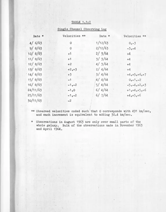
All the systematic observations of NGC 5236 were made with the

single channel receiver described in the next section. Table 1.1:I is

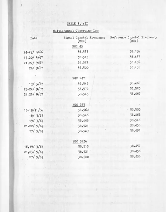
a log of these observations. Extra profiles of NGC 5236 and all the

work on the other galaxies was done with the multichannel receiver

described in section 1.5. These observations are listed in Table 1 .1:II.

1.2 Single Channel Receiver

The single channel 21 cm receiver is a frequency switched two stage

parametric amplifier, using an upconverter for the first stage and a

[image:13.608.39.596.37.769.2]

TABLE

1.1:I

Single Channel Observing Log

Date* Velocities** Date * Velocities**

4/

6/63

0

_1/12/63

_0,-3

9/ a/63

0

2/12/63

-3,-4

10/

9/63

+1

~1

3/64

+4

11/ a/63

+1

3/ 3/64

+4

12( a/63

+2

4/ 3/64

+4

13/ a/63

+2,+3

2/ 4/64

+4

·

14/ a/63

+3

3/

4/64

+4 ,+5 ,+6,+

7

15/ a/63

-1

4/

4/64

0,-1

;-2

16/ a/63

-1,-2

/

5/

4/64

-5,-4,+2,+3

24/11/63

-1,0

6/ 4/64

+1 ,+4 ,+5

-

,+6

25/11/63

-1,-2

6/ 7/64

.

+4,+5,+

6

30/11/63

-2

I

**

Observed velocities coded such that O corresponds with

491

km/sec, and each increment is equivalent to adding

30.4

km/sec.

[image:14.609.20.593.17.749.2]

TABLE

1.1:II

Multichannel Observing Log

Date Signal Crystal Frequency Reference Crystal Frequency

(MHz)

(MHz)

NGC

45

24-27/ e/66

38,513

38,456

17 ,20/ 3/67

3s.515

38.457

21,22/ 9/67

38.

521

38.456

.

26/ 9/67

38,500

38.456

NGC

247

19/ 3/67

38,545

38,466

23-24/ 9/67

·

38,572

38.520

24-25/ 9/67

38.545

38 .466

NGC

253

'

16-19/11 /66

38,560

38.500

18/ 3/67

38.546

38,466

19/ 3/67

38,466

38.546

21-22/ 9/67

38.521

38.456

27/

9/67

38.549

38 .494

NGC

5236

16,1~/ 3/67

38,515

38.457

21,23/ 9/67

38.521

38.456

[image:15.610.27.601.14.745.2]

2

receiver noise temperature of

16o°K

is obtained. Robinson

(1963)

has

described the receiver in detail so it is only necessary to give a brief

description of the observing system here. An upconverter is used as

the first stage because of its wideband low-noise characteristics and

its intrinsic stability. But the low gain of

1.3

requires the following

stage to have a low noise figure and very high gain. This is supplied

by a fixed frequency degenerate parametric amplifier, which because

of its high gain has a bandpass of only

6

MHz. All tuning and frequency

switching must therefore be done with the upconverter.

Frequency tuning is obtained by adjusting the output frequency of

a 6.8 MHz.Clapp oscillator before this is multiplied up to 980 MHz to

form the upconverter pump frequency. Since the degenerate amplifier is

only sensitive to the band centered on the fixed frequency 2400 MHz,

pump and signal frequencies satisfy the relation f . +

sig f pump

2400 MHz from which it follows that any change in the pump frequency

tunes the receiver to a different wavelength. By switching at 400 Hz

between two adjustable Clapp oscillators, one of which generates the

signal band and the other the reference band, the receiver is operated

in a frequency switched mode. The output frequencies of the Clapp

oscillators are readily tuned for any desired velocity offset from the

2

1

cm hydrogen line rest frequency. With an upconverter bandwidth

between 1 db points of 150 MHz, there is effectively no limitation

imposed on the velocity range over which the receiver can be tuned, but

smaller scale structure in the bandpass makes it advisable to keep the

separation between signal and reference frequencies small. When this

is

3

MHz, the imbalance at the output of the synchronous detectors is

I

I

tunable frequency comparison switch and a stable low-gain amplifier.

To compensate for the low gain of the upconverter the degenerate

parametric amplifier is adjusted for high gain at the cost of narrowing

the bandpass to 6 MHz. Since degenerate paramps amplify both the

signal frequency and its beat frequency with the pump, there is a

folding of the spectrum about a frequency equal to half the

pump-frequency of 4800 MHz. This in combination with the 6 MHz bandpass

restricts the receiver's output to a single channel. Signal and idler

bandpasses are made to coincide by setting the central frequency of the

bandpass filter equal to 2400 MHz.

The rest of the receiver is of conventional design. A crystal

mixer is pumped at 2370 MHz to produce a first intermediate frequency

of 29.6 MHz. This is amplified and converted by a second mixer with a 140 kHz bandwidth to 3,3 MHz, before being detected, amplified by a

400 Hz amplifier, synchronously detected and then integrated. The

output is fed to a pen recorder. As the amplifier's gain is extremely

sensitive to small fluctuations of circuit loading and pumping power,

it is necessary to ensure adequate isolation of the upconverter,

degenerate parampand mixer from each other. A three port ferrite

circulator provides 30 db of isolation for each of these stages, while

a two port isolator in the mixer line reduces feedback from the mixer.

Pumping power levels are stabilized with bias servos on the last stages

of the multiplier chains to both the upconverter and the degenerate

amplifier. These precautions enable long-term drifts in the receiver's

output to be held to less than 0.1°K/hour, while shorter term drifts

are still slow enough to allow 200 sec integration times to be used.

i

pump frequency are controlled by a common quartz crystal oscillator,

as shown in the block diagram of the receiver (Fig 1 .2:1). The

frequency of this oscillator is checked at the beginning of each

observing run with a Hewlett-Packard frequency counter, which is

accurate to one part in 107, This is also used for monitoring the

frequencies of the Clapp oscillators, which tend to drift at a rate of

6

one part in 10 per hour.

1

,

3

Single Channel Observing

4

All single channel observations of NGC 5236 consist of declination

scans. These were made in both directions along every track and have

5' declination marks inserted by the recorder's pen. Figure 1.3:1

gives a sample of a scan with a 15 sec time constant

(T

)

on the

receiver's output and a scan rate of

9

'

per minute. Using these

observing parameters, the amplitude suppression due to scanning is less

than

2'/o

from Howard's (1961) graphs. The RC rise time of the smoothing

capacitor introduces a 15 second time delay between the aerial position

given by the declination markers and the chart record of a source.

This is allowed for in reducing the observations. Both the telescope's

I

scanning rate and the chart speed are found to be constant to 0.1 •

With a receiver noise temperature (TN) of 160°K and an antenna

temperature (T) < 2°K, the r .m.s. noise fluctuation from a 140 kHz

a

filter (B) is 0.35°K from equation 1.3:1

t:, T ••••• 1 .3:1

This is reduced to 0.15°K by smoothing the scans by eye.

Whilcit observing, a check is kept on the performance of the

[image:18.604.42.594.30.770.2]

FEED

1420 Mc'

.::

-NOISE

GENERATOR

MODULA TOI,

6·8

c/s

PUMP OSCILLATOR

(SIGNAL)

FREQUENCY

COUNTER

UP -C:ONVERTER a:: w ..J c.. 1-...J :::, ~ ~LECTRONI SWITCH

400 C/S

R:tEFERENCE

<InSCILLATOR

2400

~/S

___ t BIAS 0 PUMP

j

SERVOS 6·82 Meis PUMP OSCILLATOR (REFERENCE)

-

y·

·-

--DEGENERATE AMP. BIAS 4800 MC/<;,

. . . - 1 L a:: w ..J c.. 1-...J :::, ::E CRYSTAL

OSCILLATOR

PUMP

SERVO

6·583

Mc/s MIXER a:: w ..J c.. 1-...J :::, 2370 Mc/s

PREAMP.

29· 6 Mc/s

aoo c/s GATE

D.C.

At.1P.

26·3 Mc/s

w ..J c.. 1-...J :::,

j

29. 6 Mc/s \

AMP.

MIXER

t

~

ACTIVE

FILTER

y

:ETE.~TO"

I

oo c/s

AMP.

-

l

t" JSYNCHRONOUS

1--..,--- - - ~ - - - . ! -- - -..lt..., •-. _.., ___ lDEMODULAlO ~

CHART

RECORD::R

ANALOGUE

INTEGRATOR

Sch

ematic

di

agram

o

f

du

al-

p

arainotr

ic r

eceiver

w

i

th

fr

equenc

y

s

w

itching.

i '

i

The total power is recorded with the signal as a direct check on the

receiver's performance and freedom from interference. Once in every scan the detector current is read and used to give a correction to the

gain calibration taken from a modulated noise lamp. This is used to feed a flat noise spectrum into the front end of the receiver. When modulated at 400 Hz in phase with the frequency switching it looks like

an HI signal to the receiver. The lamp is only used at the beginning and end of an observing period as the receiver's long term gain is stable and free of zenith angle effects to 0.1°K,

Calibration of MNL Once in every run the modulated noise lamp

(MNL) is compared with the continuum source 3C 353. On each occasion

5

3C 353 is scanned in right ascension and declination to get the position

of the peak deflection. A value of 57 + -3 f .u. was used for the flux of 3C 353, this vaiue being based on the absolute flux measured by

Findlay et al.,(1965) for Cassiopeia A and the ratio between this and

3C 353 measured by Goldstein (1962) and by Heeschen and Meredith (1961).

The lamp shows a variation of the ratio Temp 3C 353/Temp MNL of less

than ryfo between runs.

Beam Parameters 3c 353 was used to determine the aerial response

of the main beam, which is effectively circularly symmetric and is

well represented by

f(e)

K, exp- -

(

-

e )

2

11.5

where

e

is the angular distance from the beam axis in minutes of arc.

I

I

'

6

(defined in equation 2.3:5) is 0.58,

1 .4 Construction of Velocity Profiles

To facilitate a comparison with the observations made with the multichannel receiver the scans are processed to produce a set of velocity profiles. This requires (a) A separation of the signal due

to the source from the background radiation with a baseline, and

(b) The low frequency noise passing the output capacitor to be smoothed

by hand. When making the observations the declination scans are

continued beyond the confines of the galaxy to enable a baseline to be

determined. This is always approximated with a straight line. In the

10 minutes required to complete a scan slow fluctuations can make the

position and shape of the baseline uncertain. As the errors incurred

in drawing baselines can increase or decrease the signal observed,

their effect is reduced by averaging the forward and reverse scans and

by duplicating scans wherever possible. A weak correlation can be

expected between adjacent velocity profiles constructed from the same

set of scans. This does not appear to have affected their

interpretation, as all important features are verified by velocity

profiles taken with the 48-channel receiver.

Some care is needed in drawing the smoothing curves that reduce

the effect of the longer period noise fluctuations. These curves are

drawn to balance both positive and negative excursions from the mean,

and to remove sudden changes of profile shape whenever these occur

I

within distances < 5 • A partial check on the method is to compare

the areas under the original and the smoothed scan. These agree to better tPan 5% wherever the peak temperature is greater than 1/2°K.

i I

I

forward and reverse scans, it is unlikely that any important error is

introduced by this procedure. Once the positions of the gridpoints

along a scan are marked, it is simple to read off the signal

strength at each gridpoint. This measure is scaled with the scan's

gain calibration, averaged with all other measures made on the same

day at the same velocity and position, and plotted on the appropriate

velocity profile. All measures taken from the scans are given equal

weight, but the averages coming from two, three and four measures are

plotted with different symbols.

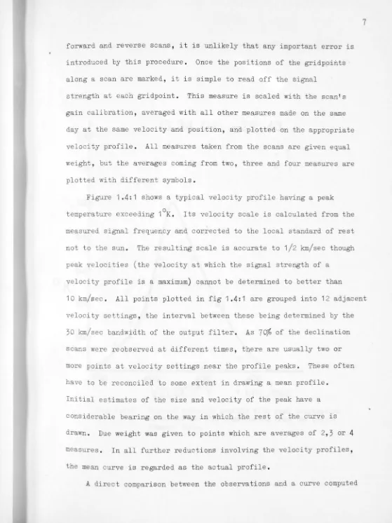
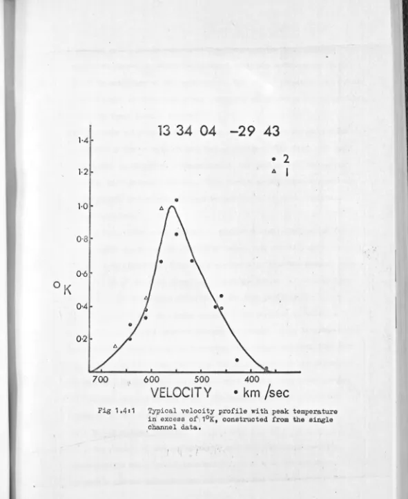
Figure 1.4:1 shows a typical velocity profile having a peak

temperature exceeding 1°K. Its velocity scale is calculated from the

measured signal frequency and corrected to the local standard of rest

not to the sun. The resulting scale is accurate to 1/2 km/sec though

peak velocities (the velocity at which the signal strength of a

velocity profile is a maximum) cannot be determined to better than

7

10 km/sec. All points plotted in fig 1.4:1 are grouped into 12 adjacent

velocity settings, the interval between these being determined by the

30 km/sec bandwidth of the output filter. As

701/o

of the declination

scans were reobserved at different times, there are usually two or

more points at velocity settings near the profile peaks. These often

have to be reconciled to some extent in drawing a mean profile.

Initial estimates of the size and velocity of the peak have a

considerable bearing on the way in which the rest of the curve is

drawn. Due weight was given to points which are averages of 2,3 or

4

measures. In all further reductions involving the velocity profiles,

the mean curve is regarded as the actual profile.

A direct comparison between the observations and a curve computed

[image:23.602.33.592.22.768.2]

1

·4

1·2

0

·2

700

13

34 04 -29 43

•

600

500

VELOCITY

• 2

A

I

400

•km/sec

Fig 1.4,1 Typical velocity profile with peak temperature

[image:24.644.38.629.16.739.2]

8

from some model galaxy would test the shapes of the mean profiles,

though the number of variables involved cause the model curves to be

almost as arbitrary as the mean curve. The only alternative is to look at the degree of self-consistency exhibited by the whole set of profiles. There are three partial checks.

(1) The peak velocity of each profile is plotted over the galaxy and contoured; a few velocities are then at variance with rest. If the mean curves could not be redrawn easily, the profile was reobserved

with the multichannel receiver. This always corroborated my previous

expectations, and showed the peak velocities to be self-consistent to ~ 10 km/sec.

(2) The area under every profile is plotted against declination for a given right ascension; the resulting curves vary smoothly from the

central peak outwards. Three measures deviated from the general rule by up to

':f/o

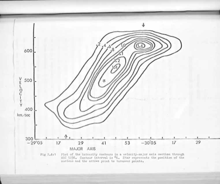
of the peak intensity. Thus the derived HI distribution is relatively independent of error in the mean profiles.

(3) In figure 2.4:1 the signal intensity has been contoured for a velocity - major axis section through the galaxy. Such diagrams are equivalent to contouring the intensity of a single spectral line with the slit parallel to and overlying the whole length of the major axis.

To draw the diagram, the intensities must be read from every portion of the mean major axis profiles. The smooth variation of all the contours in the figure exhibit a high degree of self-consistency. 1

.

5

The 48 Channel Receiver

The version of the multichannel receiver previously used for

observing the Magellanic Clouds was described by McGee and Murray

(1963)

.

9

to back it up. It did not have sufficient sensitivity to look at

galaxies outside the local Group. In August 1966 M.W,Sinclair installed

a new quasi-degenerate parametric amplifier (paramp) in front of the

existing crystal mixer. Initially the resulting receiver has a noise

temperature of 800°K, but this was improved in September 1967 to a

0

value of 350 K. Using equation 1,3:1 the noise fluctuation of the

37 kHz filters with eight minutes of integration is 0.26°K. If adjacent 0

filter outputs are averaged, this can be reduced to 0.15 K.

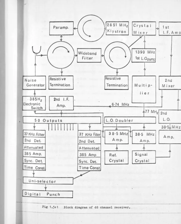
Figure 1,5:1 shows the schematic layout of the receiver used for

these observations. A circular feed horn at the focus of the 210 ft

telescope is used to feed the paramp via the first port of a four port

circulator. With the mixer connected to the third port the paramp is

effectively isolated from all the following stages by 40 db. It is

pumped at 2851 MHz with a klystron which is phase-locked to a quartz crystal oscillator by a Hewlett-Packard synchroniser. The pump power

is servo-controlled to a constant level, By using 2851 MHz to pump the

paramp, the frequency about which the spectrum is folded (1426 MHz) is given a

5

MHz offset from the 21 cm rest frequency. This is equivalent

to a blueshfft of 1000 km/sec, The idler frequencies are then

blueshifted to more remote velocities, where they are not expected to

encounter any line radiation.

In this receiver the frequency switching is done at 385 Hz on the

1388 MHz first loc~l oscillator frequency of the crystal mixer. Both

signal and reference frequencies originate from 38.5 MHz crystal-driven

oscillator units. As these are temperature controlled they are capable

of a stability of one part in 107 for extended periods. It is the

[image:26.648.20.614.23.768.2]

-C

•

Pa ramp.

_~

_f

2851 MHz

Crysta

I

_re

1 st

.

_Klystron

M ix

er

I. F. Amp

.

1

0~~

-MHz

-J,

( \

Wideband

~

~

I

1st L.Opum

~

,17

..

'

Filter

j~

+

t

A.

Noise

Resistive

Resistive

2nd

Generator

Termination

Termination

Multi p-

_Mixer

Ii e

r

,

385Hz

2nd

I.

F.

~17 ,:!>

Electronic

_Amp.

A

6•74

MHz

Switch

~

v

l.

i~77

MHz

_2nd

T

5

0

Outputs

L. 0. Doub

I

er

L.O.

11111 1111

t

I

38

·

5

MHz

..1.

r,i. _'17

37 KHz. Filter

37 KHz Filter

3

8·5

MHz

38·5

MHz

Amp.

....

-2nd Det.

_{2nd Det.}

A

n:1

p.

_Amp.

/ltt enua t ed

_Attenuated

₊

"~

385

Amp.

₃₈₅

_Amp

_Ref.

_Sig

_{_}

_nal

Sync.

Det.

_{Sync. Det.}

Crystal

Crystal

·

_{Time Const}

_{Time Const}

Uni-selector

~

Dig i ta I

Punch

- - - . - - - 1

[image:27.641.12.620.14.769.2]

switched, so that all the multiplying stages from 38.5 to 1388 MHz are

shared by both frequencies. Servos are still needed to maintain the

average mixer current during the two halves of the switching cycle at

the same level, and to maintain the total mixer current at a constant

level. When all the servos are working the baseline formed by the

48 channels is fairly stable and free of zenith angle effects. This was only the case for the September 1967 run.

10

The 31 .8 MHz intermediate frequency (I.F.) generated by the crystal

mixer is amplified before being mixed with an additional 38,5 MHz

output of the signal oscillator to produce a 2nd I.F. of 6,74 MHz.

This is fed to a bank of 48 doubletuned LC filters. These have been accurately tuned at intervals of 33.2 kHz across the 2nd I.F. All the filters have a 3 db bandwidth of 37 kHz. Careful checking over a number of years has shown a typical filter error of only ±,5 kHz

( =

.1 km/sec). After amplification, detection and synchronous detection

the output of each filter is passed to a two stage RC integrator, whose

voltage level is read out at two minute intervals to be fed to a pen-recorder and a papertape punch. Ful1 details of the digital recording have been given by Hindman et al., (1963), A second punch

was used to record the position and time whenever the telescope's

position was changed,

The receiver is tuned to a different wavelength by changing the

crystals driving the signal and reference oscillators. These have

to be chosen with care as the shape of the paramp bandpass causes an

imbalance between the signal and reference cycles. This in turn gives

rise to a slope in the baseline and a d.c. offset of all the channels

11

minimised with a 2.5 MHz difference between the signal and reference

frequencies. The closest edges of the two observed bands are then

separated by 100 km/sec and the band centres are separated by 440 km/sec.

The d.c. offset is

-2°K

.

No trouble is to be expected from the first local oscillator images at 1356 and 1496 MHz as these are subject to

10 db of attenuation by the paramp passband.

3C 353 was used for calibrating this observing system, which has

1

a half power beam width of 14.5, an effective solid angle of 238 sq mins

and a beam efficiency of Q.8.

1. 6 Multichannel Observing ·and' Reduction

As the majority of the signals being detected are of the order of

.

5°K

the method of observing adopted with the multichannel receiver has

been to integrate at a single position in the galaxy for eight minutes.

Four minutes are allowed to elapse unrecorded after every change of telescope position to let the output time constants lose their 'memory'

of the previous position. Velocity profiles are generated in reaucing

the data, by subtracting the signal profiles observed at a reference position outside the galaxy from the signal profiles of the source

itself. This would only require an occasional reference position to be

observed if the baseline were stable to

-±o

.

2°K

.

But experience has

shown that reasonable results are only obtained if the source profiles can be compared with reference profiles taken at closely comparable

times and zenith angles. It has been the uniform practice in all runs

after August 1966 to observe a reference position after every two grid

-points. Even so the baseline is still subject to abrupt intensity

usually recognised by comparing the signal profiles separately with

each of the adjacent sets of reference profiles. Some of the velocity

profiles presented in figs (3.4:1) and (3.5:1) show signs of these

perturbations.

A record of the total power was also taken with most of the

12

observations, as it gave a direct warning of any equipment malfunction

or of any electrical interference. In setting the receiver up at the

beginning of every run, the pump frequency of the klystron was measured

to check that it had not drifted significantly.

Reference Regions These were usually taken 12 minutes of right

ascension East or West of the last observed gridpoint. No HI outside

the velocity range O - +50 km/sec was ever encountered at these

positions.

Signal and Reference Frequencies In frequency switching the

receiver is made sensitive to both a signal and a reference range of

velocities. These are 340 km/sec wide and their closest edges are

separated from one another by ,..,_, 100 km/sec when the frequency

difference is - 2.5 MHz. The signal frequency is chosen to centre the

expected signal in the signal band as this simplifies the reductions

by allowing the baseline to be determined unambiguously from the

channels near the start and finish of the profile. Special care is

needed with galaxies having a wide range of velocities, since a signal

frequency must be selected for each side of the minor axis. It is

usu.ally possible to avoid a signal in the reference band by placing

this band on the high velocity side of the galaxy, where it will miss

the ~ource's signal and is well outside the range of galactic velocities.

the reference band may be sensitive to HI from the opposite end to that

being observed. This situation occurred in observing the low velocity

side of NGC

253

.

Several profiles close to the minor axis with peak

velocities near 100 km/sec show an apparent 1_absorption1 _{line at}

-100 km/sec. This is due to the observation by the reference band

13

of HI at velocities around 400 km/sec. Observations made with different

crystals show no HI at negative velocities in this part of the sky.

Gain Calibration An argon noise lamp mounted at the focus feeds

a flat noise spectrum via a probe into the circular horn. When the

lamp is modulated at

385

Hz in phase with the switching frequency, the

noise looks like line radiation to the receiver and is seen equally in

all channels. The response of every channel to a common signal is

used to calibrate the individual channel gains. Whilst the receiver's

adjustment is left unaltered, a gain calibration every

5

or

6

hours

is sufficient.

Frequency Measurement The crystal oscillator frequencies were

measured every hour with a Hewlett-Packard valve counter. This was

calibrated in September 1967 against a solid state counter which had

been standardized by the National Standards Laboratory in Sydney. Small

corrections were necessary to the frequencies measured in this run, but

the peak velocities so determined show no systematic difference from

those previously measured. The velocity scale is thought to be accurate

to 0.5 km/sec, as the velocity of the first channel in km/sec is

calculated from the measured frequencies in kHz entered in Table 1.1:II

where f ff t = 5.94 MHz and usually f₂ d

1 0

=

f . • o se n • . sig

Reductions After being checked for punching flaws the data tapes are read onto magnetic tape. A few profiles taken at random from each run were checked against the chart record of the same profile. They all matched perfectly. Before further processing the profile data is

correlated with the telescope position and time and the velocity

calculated for the first channel from the measured signal frequency is corrected to the local standard of rest. The task of applying the channel gain calibrations and calculating and plotting the velocity profiles is handled by a C.D.C,3200 computer using standard C.S.I.R.O.

programmes.

14

Each signal profile is compared with the reference profile

immediately preceding and succeeding it in time. The most representative

CHAPTER TWO

THE DISTRIBUTION AND MASS OF NEUTRAL HYDROGEN

Introduction

Most surveys of the HI distribution in our Galaxy have sought to

interpret the observations in terms of spiral structure. If this kind

of approach has a realistic base the HI arms may extend into regions

well beyond those delineated by OB stars and HII regions. Observations

of other galaxies are not readily interpreted in terms of spiral

structure, though this may largely be due to the effects of beam

smoothing. It is quite likely that different types of galaxy have

different kinds of HI distribution. Thus in the Magellanic Clouds much

of the HI is associated with large HI complexes which are distributed

at random over the surface of each galaxy. Each complex, consisting of

many HI clouds is embedded in a more general distribution of HI which

in the case of the LMC has a hole in it surrounding the optical bar.

Observatjons of all other galaxies suffer in varying degrees from

a lack of resolving power. In the 1950's the Dutch astronomers studied

0

the neutral hydrogen distribution in M31 with a 1 beam and attempted

to correct their observations for the effect of beam smoothing. This

eventual model had a peak number density at the centre (Van de Hulst, et

al, 1957) though more modern observations with greater resolution show

that the HI in M31 has a minimum at the centre. The HI appears to be

distributed in an annulus or 'ring' with the nucleus at the centre and

the peak signal at a radius of 10 kpc. For these observations by Burke

et al (1963, 1964), Gottesman et al (1966) and by Roberts (1966) the ratio

structure though the observations of Gordon (1967) only show a 10

%

dip in the HI nwnber density at the centre.

As~"' 1 - 2 for the galaxies involved in this study, there is no likelihood of observing a central minimwn in the HI distribution. No correction is made to the data for the effects of beam smoothing. The overall distribution of antenna temperature is given in Section 2.1

16

and the mean radial variation is fitted with a gaussian in Section 2.2.

Section 2.3 is concerned with evaluating the HI mass and in deriving corrections for the effects of finite opacity and a possible variation of spin temperature with radius. Finally in Section 2.4 a search is made for any trace of an HI ring using the greater effective resolution available when T (

e,~,v

)

is considered as a function of frequency.

a

2.1 The Integrated Antenna Temperature

The simplest way of describing the HI distribution is to isolate it from the velocity field prevailing in each galaxy. This is readily done in practice by measuring the area under the velocity profiles shown in figs 3.3:1, 3.4:1, 3.5:1 and 3.6:1, which is analogous to integrating the antenna temperature T (

e,~,v)

over frequency to define

a

an integrated antenna temperature TA at each observed point according to

I

_V

T (e

_a

,

~

,

v

)

dv

Fig 2.1:1a Integrated antenna temperature contours of NGC

45.

~

Multiply contour intensities by&,ox 10 to express

in units of °K x km/sec.

-22°00

~

0

45.

•

0

es . l/')

°'

...

-

C.()

- 23°30

..

..

_"

..

12 12

46 00

I

45 00

0(1950·0)

BEAM

44 00

Fig 2.1:1 b Integrated antenna tempera~~~e

contours of NGC 247. Multiply

contour intensities by ~ b·2

0

0 0

~ ~

8

If)

~

0

0

,0

~

-25°15 25

Fig 2 .1 : 1 c

I

35 45

o

(

1950·0)

Integrated antenna temperature cofi"t.:::>U:::·s of NGC

253

.

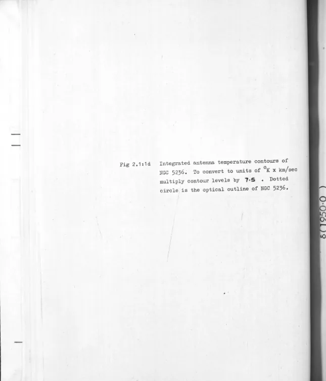
Multiply contour intensit~as

Fig 2.1:1d Integrated antenna temperature contours of

NGC 5236; To convert to units of °K x km/sec multiply contour levels by 7•5 Dotted

circle is the optical outline of NGC 5236.

[image:39.684.8.653.11.765.2]

C

-0

_.

0

~

....

~

I()

•

0

0

0

~

N

I

-0

N

0

~

N

I

0

~

°'

"'

I

0

p

0

M

I

3600

3

4

17

of the peak intensity. One check on the overall accuracy of these maps was given by three separate contour maps prepared for NGC 5236 from

progressively greater amounts of data. Though the shape and position

of the innermost contours changed a little from map to map, the mean radial variation of TA, the extrapolated HI mass and the position angle of the major axis of the HI distribution remained almost unaltered.

In figures 2.1:1a-d the nucleus is marked by a circle (o) and the HI centroid by (e). Table 2~:I lists the differences between these

1

positions. The average deviation of 2 along the major axis is too

great to be accounted for by setting errors. There is thus a considerable

degree of asymmetry in the HI distribution about the nucleus. Similar

asymmetries are observed in most of the galaxies studied with sufficient

resolution. Large deviations of the HI centroid from the nucleus are seen in both spiral galaxies such as M31, NGC 300 and the galaxies listed in Table 2.1:I and ir- irregular galaxies such as the Magellanic

1 1 1

Clouds, NGC 55 (2.5), NGC 4631 (2.5) and NGC 4656 (3 ). Since only 5 - 1c% of the total mass of a galaxy is in the form of observable HI, an

in

asymmetry in its distribution does not imply a parallel asymmetry

the distribution of the total mass.

TABLE 2.1:I

Galaxy HI Centroid

%

Asymmetry*

b.a b.b

1

45 2. 30

1 _'

247 2.8 S 27

1

253 2 .O SW 39

1 1

5236

4

.1

s

0.3

w

47

* In the sense that if the weaker end has x

%

of the total, then a 100

%

of the total= 2x + 6 • Therefore the

18

2.2 Radial Distribution of HI

Figures 2.1:1a-d all show an apparently smooth decrease of integrated antenna temperature TA with radius from the central hot spot. While

this is in part due to the smoothing of the underlying HI distribution by the beam, much of the observed decrease is real. Perhaps the

simplest method of describing the mean radial variation seen in these figures is to plot TA against an effective radius defined by

r* = / (A(TA)/n) where A(TA) is the area within the contour level TA. The data for NGC 45, 247, 253 and 5236 is plotted in fig 2.2:1 together with the least square gaussian fitted to each set of data. For ease of

comparison, the intensities are normalized at r* = 0 and the radii are expressed in kpc. The fitted gaussian represents the data easily over all radii ~ 1 kpc. Only the last one or two points from the outermost contour are poorly fitted, and in these cases the fitted

curve may underestimate the signal by up to 3afo. Figure 2.2:2 shows the gaussians fitted to the galaxies studied with the 210 ft telescope. As they are all at comparable distances and have similar optical sizes,

the effects of beam smoothing are equally severe in each case.

NGC 5236 obviously has a much more extended HI distribution than any of the other galaxies, and the signal is relatively lower at its centre.

The similarity of scale size among most of the other objects is in part due to their large values of i .

Following the method outlined in Section 6.4 the fitted dispersion a* is approximately corrected for the effects of beam smoothing by using the equation

a

_corr.

=

I

(a

_* 2 -

a

_beam2 ) _· This is sufficient to

enable the values of a obtained with different observing systems corr.

1 300

2 3109

3 253

'

55

5 2'7

6 '5

7 55

8 300

9 5236

10 20 30 ,o

R(k~)

Fig 2.2:2 Comparison of radial distributions of HI in galaxies studied at Parkes.

Dotted curves are fits to convolved optical isophotes.

l

\

\

10

Fig 2.2:1

1 • 253

2 • 2'7

3 • '5

' 05236

20 30 ,o

R(kpc)

Comparison of fitted

circularly symmetric disk with a constant T it follows from the _s

definition of r* that a _corr.

inclination by the relation a

r

is adjusted for the effect of the

a ./ cos i.

corr. a r is then the

19

dispersion or characteristic radius of the HI distribution in the plane

of the galaxy. "This is described by the gaussian

N

0 exp [~:

2

zj

r

where NH(r) is the number of HI atoms per square centimeter. Use is

made of this relation and the tabulated values of a in Chapter Four_r .

Both a and a are given in Table 2.2:I for all galaxies with corr. r

published contour maps. In the case of M31 the gaussian which is only

fitted to the outer continuous contours is rather artificial as the HI

distribution is known to be ring-shaped.

The gaussians fitted to the optical isophotes of NGC 55 and

I

NGC 300 after these had been convolved with a 13.5 beam are plotted

as dotted curves in fig 2.~:2. They show a more rapid decrease of

signal intensity with radius than the equivalent HI curves.

Quantitatively this is seen in the ratio a*(optical)/a*(HI) of 0.83

and 0.46 for NGC 55 and 300 respectively. As optical isophotes are

not available for many of the galaxies studied at 21 cm, a more general

comparison of the optical and HI sizes is given by the ratios

2a /D and 2a/D in which Dis the optical diameter of the major

corr.

axis. These ratios are entered in Table 2.2:I using the value of D

listed in column 12 of the B.G.C., since these values are already on a

consistent system and have been adjusted for the effects of inclination.

Both of these ratios show that the HI distribution is at least twice

T

A

BL

E

2

.

2

:

I

2

a

2a

.0

Galaxy a a corr r l

corr r

-D D

,

I

4

5

5

.

2

6

.

9

1.41

1

.

86

₅₅

t t

55

6

.4

(21

.

7)

0

.

88

2

.

99

(85)

I

22

4

23

.

6

5

1.

9

o

.4

7

1.

04

78

t t

2

4

7

4

.

5

7

.4

0

.

65

1.

07

68

I

,

253

3

.

7

6

.

8

0

.

52

0

.

96

73

,

,

300

7

.

6

9

.

5

0

.

87

1.

09

50

I

,

925

3

.

2

7

.

7

0

.

9

4

2

.

26

80

,

(

22

.

3

)

(5

.

87

)

(85)

3

109

6

.

6

1.

7

4

,

,

4

63

1

4.

2

14.

1

1

•

14

3

.

81

85

,

4

656

4. 1

1.41

I I

20

2.3 Mass of HI

Provided the optical depth (

T

)

is small the number of neutral

hydrogen atoms NH in a 1 cm 2 column along the line of sight can be

found without knowing the spin temperature using the well-known formula

CD

3.87 x 1014

J

Tb(\)) d\i

0

•••••••••• (2.3:1)

where Tb (

\!

)

is the brightness temperature of this element of the

source at the frequency

\!(Hz)

.

By summing over the whole projected

image of the galaxy, the total number of HI atoms is

••••.•..•• (2.3:2)

where e,cp are angular coordinates. Since Tb is not directly observed,

it is necessary to express equation (2.3:2) in terms of the antenna

temperature (T ). This is the quantity measured by the receiver, being

a

simply the average brightness temperature seen by the beam weighted

with the aerial response. If the effective area presented by the

antenna at an angle ( s,~) to the principal axis of the beam is A( s,~)

then T ( e,cp) is

a

T (9,cp)

a

••••••••••• (2.3:3)

When the antenna temperature is integrated over the whole region (c) of

convolution of the galaxy with the beam, it can be shown that

I

T (9,cp) d9dcp

C a

=

l

2

f

I

Tb(e,cp)d9dcp

I

I

A(s,~)dsd~

i galaxy beam •••••• (2•

₃

:4)

This is simplified by defining a beam efficiency

(

x

)

following

X 1

"-2

I

I

_beam A Cs,~) dsd~ •••••••••••• (2.3:5)

We get a suitable expression for the integrated brightness temperature

by substituting (2.3:4) and (2.3:5) into equation (2.3:2).

Then:--1

('If

3

.

87

X

j

Ta (e,~,v) d9d.cpdv •••••. (2.3:6) C

The HI mass is given by equation (2.3:7) after the conversion of the lefthand side from angular to linear coordinates

= 3.1on2

x-

1

III

Ta (e,~,v) d9d~dv •••.•• (2.3:7) C

where Dis the distance to the object expressed in kpc.

Equation (2.3:7) is evaluated in three stages

(1) By integrating each velocity profile over frequency to obtain the integrated antenna temperature TA. (2) By contouring TA over the plane of the sky and measuring the area inside each contour A(TA).

(3) Combines the two separate integrations over frequency and space by

measuring the area under the plot of TA versus A(TA). This determines the HI mass within the outermost contour. It is extrapolated to

infinity using the radial distribution determined in section 2.2

according to:

-where r* is the effective radius of the outermost contour. The

derived HI mass is increased by -ry/o. Both extrapolated and unextrapolated masses are listed in Table 2.3:I.

A useful check on these masses is provided by a comparison between

TABLE 2.3: I

Galaxy Unextrapolated Extrapolated T

%

* _D

NGC _{~I x 109~ ~Ix 109M}

0

Max

Difference (Mpc)

45 0.76 0.82 _{'""'.09 4.5 3}

247 1.4 _{1.47 '"'-'.19 9.8 3}

253 1 , 0 _{1.04 '"'-'.19 9.8}

3

5236 13.4 13. 9 - .10 5.0 ₅

-T * using c _{= TM /( 1 - e} Max)

ax

TABLE 2.3:II

Galaxy D 210 ft Observations _{60 ft Obse~tions}

_%

_Reference

NGC (Mpc) _{~I x 109~ ~I x 10}

0

55 3 5.95 5,35 +10 2,a

247 _{3 1.47 1 • 13 +23 1 ,a}

253 3 1. 04 2.50 -141 1, b

300 _{3 5.00 4.24 +15 3,a}

3109 2.2 1. 71

1.44

+15 4,a

5236 5 13.9 9.44 +32 1 ,a

(mean)* ₊₁₉

* excluding NGC 253

1 Table 2.3:1 _{2 Robinson et al (1966)}

al (1967) , (1966)

3 Shobbrook et _{4 Van Damme}

a Epstein ( 1964) b Roberts (1968b)