doi: 10.3389/fenvs.2019.00030
Edited by:
Ricardo Villalba, Consejo Nacional de Investigaciones Científicas y Técnicas (CONICET), Argentina
Reviewed by:
Jorge Carrasco, University of Magallanes, Chile Chenghai Wang, Lanzhou University, China
*Correspondence:
Claudio Bravo [email protected]
Specialty section:
This article was submitted to Atmospheric Science, a section of the journal Frontiers in Environmental Science
Received:30 November 2018
Accepted:20 February 2019
Published:19 March 2019
Citation:
Bravo C, Bozkurt D, Gonzalez-Reyes Á, Quincey DJ, Ross AN, Farías-Barahona D and Rojas M (2019) Assessing Snow Accumulation Patterns and Changes on the Patagonian Icefields. Front. Environ. Sci. 7:30. doi: 10.3389/fenvs.2019.00030
Assessing Snow Accumulation
Patterns and Changes on the
Patagonian Icefields
Claudio Bravo1*, Deniz Bozkurt2,3, Álvaro Gonzalez-Reyes4, Duncan J. Quincey1,
Andrew N. Ross5, David Farías-Barahona6and Maisa Rojas2,3
1School of Geography, University of Leeds, Leeds, United Kingdom,2Center for Climate and Resilience Research,
Universidad de Chile, Santiago, Chile,3Department of Geophysics, Universidad de Chile, Santiago, Chile,4Instituto de
Ciencias de la Tierra, Facultad de Ciencias, Universidad Austral de Chile, Valdivia, Chile,5School of Earth and Environment,
University of Leeds, Leeds, United Kingdom,6Institut für Geographie, Friedrich-Alexander-Universität Erlangen-Nürnberg,
Erlangen, Germany
Recent evidence shows that most Patagonian glaciers are receding rapidly. Due to the lack of in situ long-term meteorological observations, the understanding of how glaciers are responding to changes in climate over this region is extremely limited, and uncertainties exist in the glacier surface mass balance model parameterizations. This precludes a robust assessment of glacier response to current and projected climate change. An issue of central concern is the accurate estimation of precipitation phase. In this work, we have assessed spatial and temporal patterns in snow accumulation in both the North Patagonia Icefield (NPI) and South Patagonia Icefield (SPI). We used a regional climate model, RegCM4.6 and four Phase Partitioning Methods (PPM) in addition to short-term snow accumulation observations using ultrasonic depth gauges (UDG). Snow accumulation shows that rates are higher on the west side relative to the east side for both icefields. The values depend on the PPM used and reach a mean difference of 1,500 mm w.e., with some areas reaching differences higher than 3,500 mm w.e. These differences could lead to divergent mass balance estimations depending on the scheme used to define the snow accumulation. Good agreement is found in comparing UDG observations with modeled data on the plateau area of the SPI during a short time period; however, there are important differences between rates of snow accumulation determined in this work and previous estimations using ice core data at annual scale. Significant positive trends are mainly present in the autumn season on the west side of the SPI, while on the east side, significant negative trends in autumn were observed. Overall, for the rest of the area and during other seasons, no significant changes can be determined. In addition, glaciers with positive and stable elevation and frontal changes determined by previous works are related to areas where snow accumulation has increased during the period 2000–2015. This suggests that increases in snow accumulation are attenuating the response of some Patagonian glaciers to warming in a regional context of overall glacier retreat.
INTRODUCTION
Patagonia is the largest glaciated area in the Southern Hemisphere outside Antarctica. Patagonian glaciers show a strong sensitivity to climate variations and recent evidence shows that most of these glaciers are receding rapidly (Davies and Glasser, 2012; White and Copland, 2015; Meier et al., 2018). This deglaciation process is a matter of concern due to their observed and potential contribution to sea level rise (Rignot et al., 2003; Willis et al., 2012; Gardner et al., 2013). Despite this, only a few studies have focused on understanding how glaciers are responding to changes in climate over this important region of the Southern Hemisphere (Pellicciotti et al., 2014; Malz et al., 2018). The main reason for the lack of research studies over this region is associated with the scarcity of in situ long-term meteorological observations, especially on the plateau of both icefields, where extreme weather conditions prevail throughout the year.
Previous studies have focused on comparing surface elevation changes during recent decades derived from digital elevations model (DEMs) obtained from topographic and satellite data in both the North Patagonia Icefield (NPI) and the South Patagonia Icefield (SPI). Overall, these analyses show surface lowering in almost all the NPI, with some exceptions in the accumulation zones (Rivera et al., 2007; Dussaillant et al., 2018; Foresta et al., 2018). Meanwhile, negative changes are concentrated in the northern sector of the SPI (Foresta et al., 2018; Malz et al., 2018), whereas the south-central sector shows near balance conditions and even positive changes in elevation (e.g., Pío XI Glacier). As might be expected, the highest negative trends are concentrated in the ablation zone of the glaciers. The heterogeneity in glacial elevation changes reveals a complex spatial structure of the glacier responses in this region. The overall observed negative changes in surface elevation contrast with surface mass balance models studies that largely illustrate positive trends on both the NPI and SPI (Schaefer et al., 2013, 2015; Mernild et al., 2016b; Weidemann et al., 2018). One explanation suggested for this discrepancy is increasing ice flow velocities associated with ice loss due to calving. Unfortunately, to date there are no empirically-based studies of the meteorological conditions over both sides of the Patagonian Icefields that can constrain the mass balance modeling studies. Due to the lack of observation-based analyses, high uncertainties exist in the glacier surface mass balance model parameterizations precluding a complete validation of the simulated accumulation (Villarroel et al., 2013) as well as a robust assessment of the response of the glaciers to projected climate change.
Despite recent and past efforts, one of the main components of the glacier mass balance, the snowfall and hence the snow accumulation in Patagonia, remains poorly understood. Snow accumulation has been estimated at different scales from Global and Regional Climate Models (Schaefer et al., 2013, 2015; Lenaerts et al., 2014; Mernild et al., 2016a; Weidemann et al., 2018) to point scale estimates from stake observations (Rivera, 2004) and ice core data (Yamada, 1987; Matsuoka and Naruse, 1999; Shiraiwa et al., 2002; Schwikowski et al., 2013). Considering the spatial extent of both Patagonian Icefields, ice cores and
stake estimates are only representative of local conditions. Furthermore, the lack of observed accumulation data causes high uncertainties in the simulations regarding the glacier-wide amount of solid precipitation. For example, using a mass balance model for Tyndall and Gray glaciers on the SPI,Weidemann et al. (2018)showed that the accumulation values are significantly lower than those estimated by Mernild et al. (2016b). These discrepancies in the estimations are partially associated with atmospheric forcing fields and different precipitation schemes used in the mass balance models.
The accurate estimation of precipitation phase is an issue of central concern regarding the uncertainties of mass balance models. To calculate accumulation in Patagonia, the precipitation phase has been parameterized using air temperature as the input for typical Phase Partitioning Methods (PPMs) such as static threshold (e.g., Rivera, 2004; Koppes et al., 2011) and linear transition (e.g., Schaefer et al., 2013, 2015; Weidemann et al., 2018) methods. However, recent studies have shown that precipitation phase is not only a function of surface air temperature, but is also influenced by relative humidity, wind speed, stability of the atmosphere, and interaction between hydrometeors (Behrangi et al., 2018 and references therein). According to Harpold et al. (2017), the first step toward improved hydrological (and glaciological) modeling in areas with a mixed precipitation phase such as the NPI and SPI, is to educate the scientific community about current techniques and their limitations and to highlight the areas where research is most needed.
Given the general lack of data and analysis on accumulation estimates and thus associated uncertainties, as well as its relevance to understanding snow accumulation processes on the Patagonian Icefields, the main goal of this work is to analyze snow accumulation over the period 1980–2015 using a regional climate model simulation (RegCM4.6, at ∼10 km spatial resolution) and short-term on-glacier accumulation observations. In the first section, we compare the results of four PPMs, three of them previously used in the region. In the second section, we analyze the seasonal trends in snow accumulation over the period 1980–2015. In the third section, we compare the datasets with the in situ observations and previous estimates made in the scientific literature. Finally, the results are discussed in terms of the implications for glacier surface mass balance modeling and the observed glacier response.
MATERIALS AND METHODS
Study Area
The study area includes the two largest temperate ice masses located in the Southern Hemisphere: the North Patagonia Icefield (NPI) and the South Patagonia Icefield (SPI) (Figure 1). The NPI extends from 46◦30′S to 47◦30′S (Figure 1B), stretching
FIGURE 1 | (A)Regional climatic setting over the Patagonian region. Colors correspond to the predominant Köppen-Geiger climate classification for Patagonia (Beck et al., 2018) and the red rectangle corresponds to the study area.(B)SRTM topography at 1 km resolution of the study area and locations of some glaciers mentioned in the text, and(C)localization of the observations (Ultrasonic Depth Gauges) used in this work. The satellite image was acquired by Landsat 8 (OLI) on the 8 April 2014.
Mount San Valentin. It is composed of 38 glaciers larger than 0.5 km2(Dussaillant et al., 2018).
The SPI spreads over 350 km between the latitudes 48◦20′S
and 51◦30′S (Figure 1B), and is the most glaciated zone of
the Andes, covering an area of 12,232 km2 in 2016 (Meier
et al., 2018). The SPI includes a total of 48 main glacier basins, ending mainly in fjords on the western side and in lakes on the eastern side (Aniya et al., 1996). These glaciers are joined in the accumulation zone (“plateau”), with an average altitude of 1,600 m a.s.l., and a measured thickness of more than 700 m (Rivera and Casassa, 2002) with a maximum estimate of ice thickness of∼1,250 m (Gourlet et al., 2016).
This zone is strongly influenced by frontal systems associated with mid-latitude cyclones forming over the South Pacific Ocean (Figure 1A). Given the complex terrain and extreme environment, there are a small number of meteorological stations (Garreaud et al., 2013) that only partially capture the climatology and meteorological conditions of this zone, especially at higher elevations. Data from the Climate Research Unit (CRU;Sagredo and Lowell, 2012) and from Puerto Eden weather station located in the fjord zone (49◦ 08′S, 74◦ 25′W,Carrasco et al., 2002),
show that this zone is characterized by a seasonal variation in temperature with minimum values in the winter months (∼3◦C)
and maximum values in summer (∼11◦C). South of 49◦S, the
[image:3.595.44.551.63.397.2]is associated with anthropogenic effects (Abram et al., 2014) that will potentially affect climatological trends in coming decades.
Although the southern Patagonian Andes is a relatively low-elevation mountain belt, it has an influence on the longitudinal distribution of the precipitation in the region and generates an extreme climatic gradient, leading to very humid western slopes and dry eastern slopes (Schneider et al., 2003; Smith and Evans, 2007; Lenaerts et al., 2014).Garreaud et al. (2013)
showed that the precipitation at regional scale is positively or negatively correlated with zonal wind component at 850 hPa, in the western or eastern sectors of the Andes, respectively, due to the mechanical effect of the mountain chain that forces air to ascend in the western sector (windward side). On the other hand, these conditions favor downslope subsidence, and thus lead to arid conditions on the leeward side (Garreaud et al., 2013). Given these conditions, annual mean precipitation varies between 5,000 and 10,000 mm yr−1on the windward side, while it decreases to <∼300 mm yr−1on the leeward side (Garreaud et al., 2013).
In addition to the precipitation characteristics, increases in air temperature are considered to have an impact on the mass balance (Cook et al., 2003), as these glaciers lie in the range of the 0◦C isotherm. For instance, increases in air temperature
may cause a compound effect; first, more energy becomes available for melting, and second, with a small increase in air temperature during the accumulation season, air temperature may rise above 0◦C and alter the partitioning between rain and
snow (Rasmussen et al., 2007). These changes eventually have an impact on the glacier’s net mass balance. This indicates that the Patagonian glaciers are mainly sensitive to air temperature increase, since ablation is dominated by melt (Sagredo and Lowell, 2012). It is also stated that warming is the main cause for glacier retreat over the region (Masiokas et al., 2009). Between 43 and 49◦S, a warming in the land surface temperature of
0.78◦C/per decade in the period 2001–2016 was determined
by Olivares-Contreras et al. (2018). In Southern Patagonia (∼50◦S), warming of ∼0.5◦C in the last 40 years was detected
byRasmussen et al. (2007)using NCEP-NCAR reanalysis at 850 hPa level.
Observations
We used data obtained from two ultrasonic depth gauges (UDGs) (Figure 1C). These UDGs (model SR50) were installed directly on the glacier snow surface over the plateau (CECs-DGA, 2016). In the same structure, two air temperature sensors were also installed at an initial height of 2 and 4 m above ground level. Data obtained at 15 min time steps from these stations, referred to as Glacier Boundary Layer (GBL) air temperature stations (GBL1, GBL2 in Figure 1C and Table 1), are used to validate and compare snow accumulation against the estimated values obtained with the different PPMs (next sections). First, we separate the data between accumulation and ablation, before visually filtering the SR50 data to discard outlier values. Then, a moving average at hourly scale was applied in order to reduce the noise. Finally, the hourly data in meters was converted to mm w.e. using the method of estimation of density (ρs) ofHedstrom and Pomeroy (1998)based on air temperature (Ta) only:
ρs=67.92+51.25e(Ta/2.59). (1) Based on these results, we were able to estimate the daily accumulation.
Data Compilation
We compiled snow accumulation estimates of the Patagonian Icefields from previous studies to compare with the snow accumulation estimations performed in this work. Some studies measured the ablation and accumulation using short-term direct observation through the use of stakes. There is a lack of long-term mass balance measurements using the glaciological method on the NPI and SPI. In view of this fact, we also considered ice core and modeling estimations in this study.
We also compiled glaciological data related to observed glacier changes mainly between 2000 and 2015 in both the NPI and SPI. In the current study, these data obtained at glacier scale are used to support our analysis of glacier response and its implications. The compilation corresponds to elevation changes in the SPI during the period 2000–2015 (Malz et al., 2018), elevation changes in the NPI during the period 2000–2014 (Braun et al., 2019), ice velocity in both Icefields (Mouginot and Rignot, 2015), frontal changes in the SPI (Sakakibara and Sugiyama, 2014), and estimation of the accumulation-area ratio (AAR) in the NPI (Rivera et al., 2007) and in the SPI (Malz et al., 2018). Finally, we compiled glacier characteristics from the Randolph Glacier Inventory 6.0 (RGI Consortium, 2017).
Regional Climate Model (RegCM4.6)
TABLE 1 |Details of the two UDGs at the GBL stations.
Acronym Latitude Longitude Elevation [m a.s.l.] Period
Glacier Boundary Layer Station 1 (GBL1) 48◦50′02′′S 73◦34′51′′W 1,415 17 October 2015–31 December 2015
Glacier Boundary Layer Station 2 (GBL2) 48◦51′34′′S 73◦31′37′′W 1,294 25 October 2015–31 December 2015
The simulations were performed on two domains at 0.44◦
(∼50 km) and 0.09◦(∼10 km) spatial resolutions and 23 vertical
sigma levels with a one-way nesting approach. The topography of the icefields from 10 km simulations is given in Figure S1. The mother domain has 192 × 202 grid cells covering all South America and the nested domain has 320×520 grid cells centered on Chile and southwest South America based on a Rotated Mercator projection. Initial and boundary conditions for the mother domain were provided by the European Center for Medium-Range Weather Forecasts (ECMWF, ERA-Interim) Reanalysis dataset at 6-h intervals with a grid spacing of 0.75◦
resolution. The nested domain was then forced by the 3D atmospheric outputs of the model domain at 6-h intervals. ERA-Interim sea surface temperature fields (6-h intervals, 0.75◦
resolution) were used as surface boundary conditions. The simulations were performed continuously from 1 January 1979 to 31 December 2015. The first year of simulations (1979) was selected as the spin-up period and, thus, was not considered in the analysis.
Ongoing work found that, overall, RegCM4 is capable of reproducing mean spatial fields of important large-scale features such as South Pacific Subtropical Anticyclone dry regime, westerlies over Patagonia and low-level moisture distribution along both sides of the Andes barrier. The same study also demonstrates that the simulations tend to have stronger westerlies over Patagonia and further suggest that 10-km simulation results exhibit a reasonable representation of spatial and temporal variability of temperature and precipitation. For instance, high-resolution simulation results reproduce reasonably well the observed spatial pattern of frost days with a close estimate of the observed number of days over the Patagonian Icefields.
Phase Partitioning Methods (PPMs)
To calculate and assess the snow accumulation under different schemes, four methods were used to separate between snowfall and rain. The primary input is the 10-km total precipitation simulations from RegCM4.6, as our intention is to assess the snow accumulation under four PPMs, three of them previously used in the Patagonian Icefields. In addition, 10-km simulations from RegCM4.6 of near-surface air temperature, relative humidity (at 2 m), and atmospheric surface pressure were used. In all cases, we used daily model output. In all these methods, the required inputs are air temperature and total precipitation, while in the fourth method a broader range of meteorological inputs are needed.
The first method considers a threshold value in the air temperature to separate between rainfall and snowfall. The chosen threshold temperature is 2◦C as this value was used in
studies of the San Rafael Glacier in the NPI (Koppes et al., 2011) and the Chico Glacier in the SPI (Rivera, 2004). In this article, we refer to this method as 2C. This static temperature threshold is close to that used by the BATs scheme
The second method was used byWeidemann et al. (2018)
(WE, hereafter), where the fraction of solid precipitation (r) is estimated according to:
r=0.5∗(−tanh((Ta−1)∗3)+1). (2) In this equation, the proportion of solid precipitation to total precipitation is smoothly scaled between 100 and 0% within an air temperature range of 0–2◦C, meaning that under 0◦C the
fraction of solid precipitation is 100%, while above the 2◦C the
fraction of solid precipitation is 0%. This method has been also applied to the Gran Campo Nevado Icefield in southernmost Patagonia (Möller et al., 2007; Weidemann et al., 2013).
The third method was used bySchaefer et al. (2013, 2015)
in the NPI and SPI (SC, hereafter). The accumulation (q) is the fraction of the solid precipitation which is determined by the temperature (Ta) in the grid cell(I):
q(I)=
0, Ta(I) >1.5◦C
1.5◦C−Ta(I)
1◦C , 0.5◦C<Ta(I) <1.5◦C
1, Ta(I) <0.5◦C.
(3)
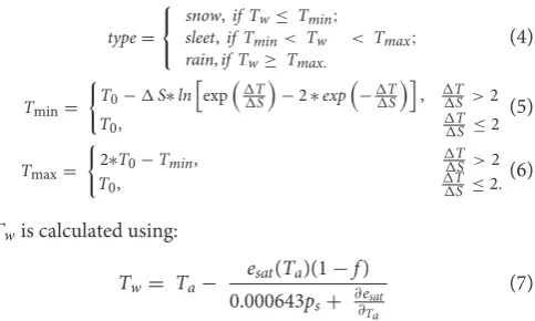
Finally, the fourth method corresponds to the parameterization proposed by Ding et al. (2014) (DI, hereafter). This scheme was constructed using climate data from China and only evaluated over China; however, evaluations for further regions are recommended (Ding et al., 2014). This scheme defines three types of precipitation (snow, sleet and rain) using minimum and maximum temperatures (TminandTmax) and the wet-bulb temperatureTw[◦C] as threshold:
type=
snow,if Tw≤ Tmin; sleet,if Tmin< Tw rain,if Tw≥ Tmax.
< Tmax; (4)
Tmin=
(
T0−1S∗ln
h exp1T
1S
−2∗exp
−11T S
i , 1T
1S>2
T0, 11TS ≤2
(5)
Tmax=
(
2∗T0−Tmin, 11TS >2
T0, 11TS≤2.
(6)
Twis calculated using:
Tw= Ta− e
sat(Ta)(1−f) 0.000643ps+ ∂∂esat
Ta
(7)
empirical equation of Bolton (1980), and ps is the surface atmospheric pressure in hPa.
The three parameters (1T,1S,T0) of this model depend not only on air temperature but also on other conditions such as relative humidity (f, ranges from 0 to 1) and the elevation of the point in km (Z):
1T = 0.215−0.099∗f+1.018∗f2 (8)
1S= 2.374−1.634∗f (9)
T0 = −5.87−0.1042∗Z+0.0885∗Z2+16.06∗f
− 9.614∗f2. (10)
1Tis the difference between the temperature of the probability threshold for snow (or snow and sleet) and the temperature of the centralized probabilities curve.1Srepresents a temperature scale in which an increase in value leads to widening of the temperature range of snow/ratio transitions. T0 is the temperature that approximately represents the center of Tw range in which snow/rain transitions happens. This method is dynamic as it is dual-threshold whenf>78% and single threshold method when
f≤78%. The complete parameterization scheme and explanation for precipitation type discrimination and data used can be found inDing et al. (2014).
To analyze the spatial differences in the snow accumulation spatial patterns and annual cycle, we divide the study area into six zones, classifying the glaciers according to their location. The NPI is separated into west (NPI W; the San Rafael and San Quintin glaciers) and east (NPI E; the Nef, Colonia, Pared Norte, Soler, Leones, etc. glaciers) while the SPI is separated into four zones, SPI north-west (SPI NW, the Jorge Montt, Bernardo, Témpano, Occidental, Greve, and Pío XI glaciers), SPI north-east (SPI NE; the O’Higgins, Chico, and Viedma glaciers), SPI south-west (SPI SW; the HPS29, HPS31, HPS34, Asia, and Amalia glaciers) and SPI south-east (SPI SE; the Ameghino, Perito Moreno, Gray, and Tyndall glaciers).
Trend Analysis
In order to identify trends in annual and seasonal snow accumulation for the four PPM in the period 1980–2015, we used two methods—linear least-squares slopes and Sen’s slope tests. The linear least-square slopes and the Sen’s slope test allow to compute the magnitude of the trend. The slope of the snow accumulation at each season and at annual scale is regressed on time and hence used to quantify temporal trends. The Sen’s slope test uses a linear model to estimate the slope of the trend choosing the median of the slopes, and the variance of the residuals should be constant in time (Salmi et al., 2002). We also estimate the statistical significance at 95% (p-value<0.05) using the Mann-Kendall test. The trend calculation is also applied to seasonal time series values of each zone [Figure 1and defined in section Phase Partitioning Methods (PPMs)] and to individual glaciers in the period 2000–2015, in order to compare with the trends in the geodetic mass balance over the same period.
RESULTS
Inter-comparison of PPMs
The spatial patterns in the distribution of annual snow accumulation are similar between the four PPM methods (Figure 2). All PPM methods driven by the data from RegCM4.6 show that the west sides of both Patagonian Icefields receive a higher amount of snowfall relative to the east side, indicating the capability of RegCM4.6 to capture the extreme orographic effect (Table 2 and Figure 2). Overall, in all the zones, the 2C method shows the highest amounts of snow accumulation, while the DI method shows the lowest values (Table 2). Interestingly, if we consider the sleet type as accumulation in the DI method, the total (snow plus sleet,Table 2andFigure S2) is of a similar magnitude to that of the 2C method. This suggests that the air temperature threshold used in the 2C method is appropriate for estimating the total rain, if we compare with the DI method. The WE and SC method are of similar magnitude at annual and season scale (Figure 2;Tables 2,S2). The interannual variability (Table 2) and seasonal scale (Table S1) is higher on the west side in both icefields. Finally, the sleet type precipitation (Figure S2) shows a higher rate on the western side of both icefields, in line with the more humid conditions that would be expected at the windward side of the Andes.
A comparison of the maximum values of each PPM with respect to latitudinal variation of snow accumulation is given inFigure 3. Maximum values reach 14,000 mm w.e. in the 2C method, the DI model reaches 11,500 mm w.e., and the WE and SC methods are around 13,000 mm w.e. at the same latitude (Figure 3). This maximum accumulation point corresponds to the HPS15, HPS19, and Penguin glaciers in the SPI. Other areas with a high amount of accumulation are the accumulation zones of the Pío XI and HPS34 glaciers, with maximum values around 12,000 mm w.e. (2C method) and 9,000 mm w.e. (DI method). For the NPI, a similar amount of snow accumulation is estimated throughout the accumulation zones of the glaciers on the west side, with values between 4,000 and 7,500 mm w.e. The maximum value in the NPI depends on the PPM used (Figure 3). For instance, 2C shows a peak value (7,000 mm w.e.) in the accumulation zone of the San Quintin Glacier (∼47◦S) while
the DI method shows maximum value on the San Rafael Glacier accumulation zone and on the Benito, HPN1, and Acodado glaciers (∼5,000 mm w.e.).
The annual mean differences between the models that give the highest (2C) and lowest amounts of snow accumulation (DI) reach a mean value of 1,626 mm w.e. in NPI W, 373 mm w.e.in NPI E, 3,542 mm w.e. in SPI NW, 823 mm w.e. in SPI NE, 2,015 mm w.e. in SPI SW and 646 mm w.e. in SPI SE (Table 2). Details of the maximum and minimum amount of snow accumulation per zone and per season are given inTable S2.
FIGURE 2 |1980–2015 annual mean value of snow accumulation (mm w.e.) for each PPM.(A)2C,(B)WE,(C)SC, and(D)DI method. Icefield contours in black were obtained from RGI consortium (2017) and edited using a Landsat 8 image (OLI) of the 8 April 2014. Coastlines are in gray.
the year, while west zones show a marked cycle in the snow accumulation. In the north-south direction, the east side zones show that the amplitude of the annual cycle is small in the SPI NE and SPI SE zones relative to the NPI E.
In summary, an overall spatial and temporal consistency exists between the four PPMs as all of them show consistently larger
TABLE 2 |Annual mean and standard deviation 1980–2015 of the snow accumulation values by zone and PPM.
Zone PPM/RegCM4.6 [mm w.e.]
2C WE SC DI DI (snow+sleet)
Mean Std Dev Mean Std Dev Mean Std Dev Mean Std Dev Mean Std Dev
NPI W 4,941 463 4,313 416 4,314 416 3,315 381 4,892 459
NPI E 1,084 107 913 98 914 99 710 92 1,084 107
SPI NW 8,010 908 6,500 796 6,500 796 4,467 641 7,883 891
SPI NE 4,186 381 3,873 358 3,874 358 3,363 326 4,166 380
SPI SW 5,471 532 4,680 492 4,680 491 3,455 436 5,408 527
SPI SE 3,033 226 2,801 215 2,801 216 2,388 201 3,027 224
FIGURE 3 |1980–2015 maximum mean value of snowfall for each PPMs.
Seasonal Trends 1980–2015
We further analyzed the seasonal trends obtained by three of the four PPMs (2C, WE, and DI) as the WE and SC methods show almost identical values and inter-annual variability. Trends obtained using Sen’s slope and linear least-square slopes are similar spatially and in magnitude, therefore in this section we analyzed the result of the least-square slope (Figure 5), while the results of the Sen’s slope are shown in the Supplementary Material,Figure S3.
Spatial heterogeneity exists in the trends, with some areas showing an increasing trend in snow accumulation while other areas show a decreasing trend or no change (Figure 5).
Overall, throughout all the seasons, areas of no significant change correspond to terrain outside of both icefields. On the icefields, areas with increasing and decreasing trends in snow accumulation are concentrated on the plateau on the west and east sides of both icefields, respectively. Statistically significant positive trends are detected on the SPI in autumn. The location of these positive trends corresponds to the plateau or accumulation zones of the glaciers. On the other hand, in the ablation zones, especially those in the north-west section of the SPI (e.g., Témpano, Bernardo, Pío XI) there are no significant positive trends, and in some areas negative trends exist. In autumn, the significant negative trends are concentrated on the east side of the NPI and on the east side of the SPI in the zones of the O’Higgins, Chico, Upsala, Viedma, Ameghino, and Perito Moreno glaciers. In these areas, negative trends are also detected in spring but the values are not significant. In winter, a predominance of positive, although not significant, trends is determined on both icefields.
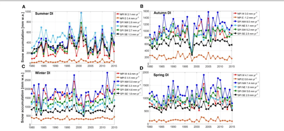
The time series of each zone are similar between the PPMs and [see section Phase Partitioning Methods (PPMs)] shows an important inter-annual variability. For instance, for the DI method in autumn (Figure 6), the generally positive trend was interrupted in 1997, with the snow accumulation values sharply dropping more than 500 mm w.e. for both icefields. Interestingly, the highest snow accumulation corresponds to the winter season of the same year, with values reaching around 3,000 mm w.e. in the west side of the SPI. Using 2C and WE methods, the winter 1998 values are close to 4,000 mm w.e. (not shown).
In summary, spatial and temporal differences exist in the snow accumulation trends. Spatially, positive trends are concentrated on the west side of both icefields throughout all seasons, while negative trends are concentrated in some areas on the east side of both icefields during autumn, winter and spring. However, in both cases significant trends are only present in the autumn season.
Comparisons With Measured data
UDG Observations
FIGURE 4 |Annual cycle of snow accumulation for the sub-regions of both Patagonia Icefields.(A)2C,(B)WE,(C)SC,(D)DI.
FIGURE 5 |Seasonal trends 1980−2015 in mm w.e. yr−1for three Phase Partitioning Methods. Points indicate statistically significant trend (p<0.05).(A)Summer, (B)Autumn,(C)Winter and,(D)Spring. Icefield contours are in black and coastlines in gray.
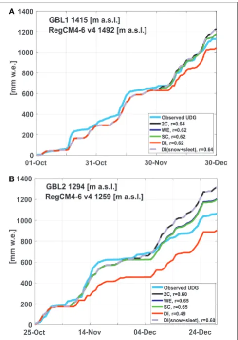
a.s.l.; the grid characteristics are considered to be closer to the GBL2 (seeTable 1). Regarding the GBL1, we used the grid point adjacent to the SW with an elevation of 1,492 m a.s.l., which is close to the real elevation of GBL1 (Table 1).
At GBL1, the PPMs show a total accumulation between 1,000 and 1,200 mm w.e. while the data from the UDG suggests an
FIGURE 6 |Seasonal time series and trends of the snow accumulation for six sub-regions of the study area using the DI method.(A)Summer,(B)Autumn,(C)Winter and,(D)Spring. The legend also indicates the annual trend.
1,300 mm w.e. while the observations suggest 1,050 mm w.e. Similar to GBL1, the r values are in the order of 0.60 and 0.65, except the one for the DI method (0.49,Figure 7). In the same location, the r value is higher (0.60) if the sleet type is considered as accumulation. Although some uncertainties may exist in estimating the accumulation from the UDGs (e.g., filter used), estimated values of the fourth PPMs using RegCM4.6 data perform well-compared to those obtained from the UDGs, especially at GBL1. The estimated values based on four PPMs are in the range of the observed values from the UDGs, but in terms of absolute values, the WE method is the most accurate at GBL1 (difference of 46 mm w.e.) while the SC method is the most accurate at GBL2 (difference of 135 mm w.e.). It is important to note that the regional climate models themselves may introduce uncertainty to the simulated variables associated with the physical configuration used in the model (e.g., radiation and cumulus schemes). Therefore, some inherent uncertainties may exist in the estimated values as well.
Previous Snow Accumulation Estimations and Comparisons
Details of the location of ice cores collected on the Patagonian Icefields are given inTable 3. These data were analyzed in order to obtain snow accumulation rates across the NPI and SPI (Table 3). Ice core data estimates an accumulation of 5,600 mm w.e at Nef Glacier in the NPI (Matsuoka and Naruse, 1999), while the estimated values based on the RegCM4.6 data are in the range of 4,100 to 5,000 mm w.e. for the same glacier. On the other hand, at Tyndall Glacier located in the SPI, differences between the ice core and RegCM4.6 estimates are even larger, reaching (in the case of the DI method) a maximum difference of 11,400 mm w.e. in the period between summer 1998 and summer 1999. Other comparisons of ice core and RegCM4.6-based estimates are given
inTable 3.In all cases, estimations using Tyndall Glacier ice core data are larger than those four PPMs using the RegCM4.6 data. The opposite relation is found when comparing the RegCM4.6-based snow accumulation values with those estimated by ice core data (Schwikowski et al., 2013) from the accumulation zone of the Pío XI Glacier (∼2,600 m a.s.l.). For instance, this ice core data estimates a mean annual accumulation of 5,800 mm w.e. (with a range of 3,400–7,100 mm w.e.) between the years 2001 and 2005. These values are not as high as others have previously estimated for the SPI. At this point, the estimate based on RegCM4.6 data illustrates a higher amount of accumulation values with differences of∼4,500 mm in 2001 and<∼800 mm w.e. in 2002. Other studies estimate a mean accumulation of 1,200 mm w.e. yr−1 in Perito Moreno Glacier of the SPI (50◦38′S, 73◦15′W,
2,680 m a.s.l.,Aristarain and Delmas, 1993), which is lower than the annual rates of the current work.
In terms of modeling snow accumulation, a recent study by
Weidemann et al. (2018)estimated the total mean precipitation for two glaciers of the SPI—the Tyndall and Gray glaciers. The precipitation distribution was modeled using an analytical orographic precipitation model at 1 km resolution, then the SC method was applied to obtain the amount of solid precipitation. The comparison of these results with those obtained in the current study for the same hydrological years is presented in Figures 8A,B. Overall, the inter-annual variability (2000–2015) between the time series of the two estimations is similar, yet there are some differences in the estimated snow accumulation values. At Gray Glacier, the annual accumulation estimated by
FIGURE 7 |Comparison of accumulated snowfall using four PPMs and observations at(A)GBL1 and(B)GBL2. The correlation coefficient (r) values of each method are calculated in comparing with the observations.
give closer values to those inWeidemann et al. (2018). At Tyndall Glacier, the estimates fromWeidemann et al. (2018)are in the range of those estimated by the four PPMs, mainly concentrated between the values estimated using the DI and SC-WE methods. Previous observations of snow accumulation using stakes are limited to short and discrete periods, and to the ablation season. For example, Rivera (2004)used three stakes located at 1,445, 1,577, and 1,833 m a.s.l., and measured values of 9,630±1,360 and 4,070 ± 540 mm yr−1 at the highest and lower stakes, respectively. The RegCM4.6-based estimates give rates in the order of 1,000 to 3,000 mm w.e. The distributions of the observed snow accumulation give an exponential relationship between precipitation and altitude, but if the precipitation is extrapolated to the higher altitudes of the Chico Glacier, the values reach 33,000 mm yr−1, which seem to be unrealistic (Rivera, 2004) and approximately three times larger than the rates estimated in the current work. It is important to note that these observations were only collected over a period of 14 to 34 days and then extrapolated to annual values.
In summary, good agreement is found in comparing UDG observations with modeled data on the plateau area of the
SPI during a short time period; however, there are important differences between rates of snow accumulation determined in this work and previous estimates using ice core and stake observation data at annual scale.
DISCUSSION
Performance of the RegCM4.6 Model and
PPMs Parametrization
Overall, at a regional scale the RegCM4.6 reproduces the main precipitation characteristics of the study area, which are dominated by extreme orographic effects. All four PPMs lead to higher amounts of snow accumulation on the west side relative to the east side. Other models have also shown similar features. For instance,Lenaerts et al. (2014) used a high-resolution regional atmospheric climate model over Patagonia (RACMO2, 1979– 2012) to show extreme orographic precipitation due to the narrow Andes barrier separating the wet windward side from the dry leeward side. Specifically, in terms of spatial differences in snow accumulation,Mernild et al. (2016b)indicated that snow accumulation at the same elevation is higher at the west side relative to the east side. Another interesting point is that sleet is higher at the west side of both icefields than that at the east side, indicating more humid and warmer conditions observed on the west side, eventually allowing for the occurrence of the mixed phase precipitation. Remote sensing observations also suggest the influence of the humid conditions on the snow facies. For instance,De Angelis et al. (2007)determined a relatively higher area of advanced snow metamorphism on the west side compared to the east side of the SPI. Outside of the icefields, in the north-east of the NPI (upper Baker River Basin),Krogh et al. (2015)
estimated that snowfall is 28.5% of the total precipitation at basin scale. This value is in the range of the fractions estimated for this region in our work (25–35%).
On the other hand, some notable differences exist when comparing the previous estimates mainly with ice core-derived accumulation with those calculated in our work. The causes of this disparity are unclear but could conceivably be associated with differences between the local conditions at the ice core site extraction vs. the spatial resolution of RegCM4.6. Furthermore, erroneous estimates from ice core data due to water melt percolation (Rivera, 2004) or a more general underestimation of snow accumulation by the RegCM4.6 can be considered for the discrepancies in estimation of snow accumulation. Regardless, these differences highlight that uncertainties in quantifying the snow accumulation still exist in this extreme environment.
TABLE 3 |Comparison of previous snow accumulation estimates using ice core data with the snow accumulation obtained in this work.
References Location Period Accumulation
[mm w.e.]
PPM/RegCM4.6 [mm w.e.]
2C WE SC DI
Matsuoka and Naruse, 1999
Nef Glacier 46◦56′S,
73◦19′W 1,500 m asl
1996 5,600 5,000 4,900 4,900 4,100
Shiraiwa et al., 2002 Tyndall Glacier 50◦59′S,
73◦31′W 1,756 m asl
Summer 1998–Summer 1999 17,800 9,000 8,100 8,100 6,400
Summer 1999–December 1999 11,000 7,700 7,100 7,100 5,300
Kohshima et al., 2007 Tyndall Glacier 50◦59′S,
73◦31′W 1,756 m asl
Winter 1998–Winter 1999 12,900 10,000 9,200 9,200 7,200
Winter 1999–December 1999 5,100 4,100 4,000 4,000 3,300
Fall 1998–Fall 1999 14,700 9,000 8,100 8,100 6,200
Fall 1999–December 1999 8,600 6,100 5,800 5,900 4,800
Schwikowski et al., 2013
Pío XI Glacier 49◦16′S, 73◦
21′W 2,600 m asl
1 February 2001−31 January 2002 3,400 8,041 7,908 7,913 7,384
1 February 2002−31 January 2003 7,100 7,593 7,444 7,450 7,275
1 February 2003−31 January 2004 5,800 9,976 9,611 9,612 8,769
1 February 2004−31 January 2005 6,500 8,723 8,489 8,504 7,852
1 February 2005−31 January 2006 6,000 8,301 8,155 8,155 7,769
Note that periods for each comparison are different.
wind speed distribution at 700 and 850 hPa levels (Figure S4). In contrast to this, the years of 2001 and 2003—with the largest differences in snow accumulation (Table 3)—had higher wind speeds at these same levels (Figure S4). Given that RegCM4 is forced by ERA-Interim, the wind speed variability can be further amplified by the regional climate model itself. Indeed, RegCM4 gives a systematic overestimation of 850 hPa zonal wind speed over large parts of the Icefields (Figure S5). These results illustrate the crucial role of local winds in controlling rates of snow accumulation, which is also indicated bySchwikowski et al. (2013)and Schaefer et al. (2015). In addition,Aristarain and Delmas (1993) also indicated the same mechanism to explain the low annual snow accumulation rate estimated in the accumulation zone of the Perito Moreno Glacier using an ice core. Thus, the derived net accumulation rates from these ice cores could represent lower limits in the snow accumulation.
In contrast, the estimated snow accumulation based on different PPMs using the RegCM4.6 data seems to agree with the observed snow accumulation, even at daily scale (r = ∼0.6), during the October-December period of 2015. One reason is that UDG measurements are at 15 min time steps, capturing the actual snow accumulation. Therefore, UDGs are not affected by the effect of wind on the snow drift after the accumulation events. The location of the UDGs on the plateau, where gentle topography is present, is likely to reduce the differences between model and observation. On the other hand, the comparison of the hypsometric curve between the topography under 10 km and at 1 km resolutions (Figure S1) shows important differences at elevations over∼1,800 m a.s.l., which correspond to around the 20% of the total area of both icefields. Therefore, the higher elevations are not represented by the topography used in the RegCM4.6 simulations, illustrating a limitation of the model, which could explain the differences between the snow accumulation determined by Weidemann et al. (2018)for the Tyndall and Gray glaciers, where a higher resolution model (1 km) was used. It is important to note
that local precipitation amount and snow accumulation depend on the correct representation of topography (Lenaerts et al., 2014). Therefore, given that ∼10 km grid resolution is not able to resolve always and exactly the complex topography in the region, the total amount of estimated snow accumulation, especially in narrow glacier valleys (e.g., Chico and Nef glaciers), steep slopes and in the ice-rock transitions of both icefields, must be taken with caution. A robust statistical downscaling or bias correction method should therefore be applied if these data are to be used to drive mass balance estimations at glacier scale.
Snow Accumulation Changes 1980–2015
Previous modeling studies have also estimated an increase in snow accumulation over annual to decadal timescale. For example, Schaefer et al. (2013) simulated an increase of accumulation on the NPI, from 1990–2011 as compared to 1975– 1990, andMernild et al. (2016a)also estimated positive trends on the plateaus of both NPI and SPI during the period 1979–2014. These trends were detected at higher elevations above∼1,200 m
a.s.l. and on the west side of the divide.
In contrast to the increased tendency of snow accumulation at higher elevations, observational-based studies focusing on the analysis of satellites images (e.g., MODIS, LANDSAT) show a reduction in snow cover area. For example,Pérez et al. (2018)
estimated a non-significant decrease in snow cover over the Aysén River Catchment located north-east of our study area (45◦–46◦S). In the south of our study region, other studies
suggested a reduction in snow cover area. For instance, further south, at Brunswick Peninsula (53◦S), results show a significant
FIGURE 8 |Comparison of annual snow accumulation using the four PPMs and estimates fromWeidemann et al. (2018).(A)Distributed mean at Gray Glacier, and(B)distributed mean at Tyndall Glacier.
scale (Lopez et al., 2008). Therefore, an overall reduction in snow-covered area does not necessarily contradict the observed snow accumulation increase at the highest elevations. It should be noted, however, that the lack of long-term records of snow accumulation in this sector of the Andes makes it difficult to reach definitive results.
Previous studies show an increasing trend of the snow accumulation over the high latitudes in a warmer climate (e.g., Thomas et al., 2017; Medley and Thomas, 2019). These changes are mainly confined to regional scales and determined by thermodynamical (e.g., moisture-holding capacity of air) and dynamical (e.g., wind speed) responses under warmer climatic conditions. Indeed, the increase in snow accumulation determined in the current work occurs under a warming trend. The fields of the air temperature from the RegCM4.6, which are used to calculate the snow accumulation, show positive trends, especially in autumn and winter (Figure S6) when larger increases in snow accumulation are determined. However, rather than the regional scale, the positive trend in snow accumulation detected in this study and previous ones is limited to the local scale, mainly concentrated at elevations over∼1,000 m a.s.l on the west side of both icefields. Lower elevation terrain shows no trend and even a negative trend in snow accumulation on the eastern side of the icefields.
The spatial differences in snow accumulation trend could be associated with the location of the study area since it corresponds
to the borders where a shift in the position of the zonal winds has been observed (Gupta and England, 2006). Indeed, an increase in the total precipitation of ∼200 mm decade−1 was observed south of 50◦S for the period 1961–2000 (Garreaud et al., 2013).
However,Garreaud et al. (2013)also indicated a negative trend in the west Andean flank lying north of 50◦S and recently, Boisier et al. (2019)also indicated a negative trend in the total precipitation based on local observations during the period 1960–2016 on the eastern side of the NPI and in northern Patagonia. These regional differences are associated with spatial differences in the tendency of the westerlies, since weaker and stronger westerlies have been detected at mid-latitudes (∼45◦S)
and around 60◦S, respectively. This opposite trend in westerlies
has been linked to the positive phase of the SAM. During this phase, a low pressure anomaly over Antarctica extends to∼55◦S with an out of phase circumpolar positive anomaly
centered at 45◦S. This pressure difference is associated with a
zonal geostrophic wind anomaly that is positive south of 45◦S
and negative to the north (Gupta and England, 2006). The positive phase of SAM has also been associated with warming sea surface temperatures in the western Pacific (Thomas et al., 2017). Hence, this is an area of transition where different temporal and spatial impacts are expected to exist. In fact, the positive trends in snow accumulation, especially in autumn and winter, tend to be larger toward the south (∼50◦S), suggesting some
influence of the dominant positive phase of SAM in the last decades (Marshall, 2003).
Spatial differences in snow dynamics are also evident in snow persistence (fraction of time that snow is present on the ground). This area is a transition zone between a dominant decrease (north of 46◦) and dominant increase (south of 50◦S)
of snow persistence (Hammond et al., 2018). In the west-east direction, SAM also influences the snow accumulation trends as the precipitation at the regional scale is positively or negatively correlated with a zonal wind component of 850 hPa in the western or eastern sectors of the Andes, respectively, due to the mechanical effect of the Andes (Garreaud et al., 2013). This effect forces air masses to ascend in the western sector (windward), favoring conditions for saturation and hence the occurrence of precipitation; on the other hand, it results in subsidence and inhibition of the precipitation in the eastern sector (leeward) (Garreaud et al., 2013). Hence, an increase in the westerly winds and moisture content associated with a dominant positive phase of SAM as well as windward precipitation enhancement (and leeward inhibition) due to orographic effects could explain the snow accumulation increase over 1,000 m a.s.l. on the western side and the reduction on the east side in the context of climate warming (Rasmussen et al., 2007; Aguirre et al., 2018; Olivares-Contreras et al., 2018).
Implications for Glacier Mass Balance
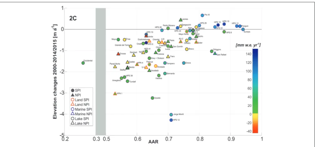
FIGURE 9 |Observed elevation changes in the period 2000–2014/2015 for both icefields vs. the accumulation-area ratio (AAR). The color represents the snow accumulation trends by glaciers using the 2C as PPM. Terminus type is also indicated depending the color of the contour for each symbol, triangle for the SPI, and circle for the NPI (see legend). Note that the x-axis is broken. Due to space issues some glaciers names are not indicated.
the use of different schemes to derive the snow/rain ratio may lead surface mass balance modeling efforts to differ considerably (Weidemann et al., 2018). This could partly explain the differences between the positive modeling mass balance (e.g.,
Schaefer et al., 2013, 2015; Mernild et al., 2016b; Weidemann et al., 2018) and the negative geodetic mass balance (e.g.,
Dussaillant et al., 2018; Malz et al., 2018) that have been documented in the literature.
Another issue to consider is if the sleet precipitation type should be considered as surface accumulation since the differences between the 2C and DI (snow plus sleet) methods are reduced considerably, especially on the western side of both icefields. Sleet is defined as a mixture of snow and rain and is associated with refreezing before reaching the ground, which forms an ice core surrounded by liquid water (Whiteman, 2000). Sleet particles are usually formed near the freezing point, where both rain and snow particles coexist (Ostrometzky et al., 2015). In this sense, it is probably valid that an undetermined percentage of sleet could be considered as surface accumulation (the ice core), while the liquid section percolates into the glacier and cannot therefore be considered as surface accumulation. It is beyond the aim of this work to define this percentage, but it seems that an accumulation in the range between the 2C and DI (snow plus sleet) and DI (snow) is a more realistic estimation. The SC and WE methods are in this range and are the closest to the accumulation estimated with the UDG observations. Other types of accumulation have been described in this zone, such as rime accretion due to supercooled water droplets transport by the strong winds (Whiteman and Garibotti, 2013); nevertheless, quantification and implications for surface mass balance have not been studied in detail to date.
At long-term scale, the increase in snow accumulation during winter months has been discussed as the cause of glacier mass balance stability and even glacier expansion in the Karakoram region (the pattern that has been termed the Karakoram anomaly;
Kapnick et al., 2014). To explore the long-term glacier response, we compare annual snow accumulation trends from this work and results from geodetic mass balance at glacier scale during the period 2000–2014/2015. Elevation change data for the SPI covers the period from 2000 to 2015 (Malz et al., 2018), whereas it covers the period from 2000 to 2014 for the NPI (Braun et al., 2019). Overall, at the glacier scale, elevation change data seem to suggest that the positive values correspond to the glaciers with accumulation area ratio (AAR) over 0.8 and classified as marine-terminating glaciers according to the Randolph Glacier Inventory (RGI 6.0;RGI Consortium, 2017). According to the data in this work, these glaciers also showed a larger annual positive trend in snow accumulation in the period 2000–2015 (Figure 9). Some exceptions exist such as Jorge Montt and HPS 12 glaciers, which besides being marine terminating glaciers, show mostly negative rates of elevation change (Malz et al., 2018). The other exception is the San Rafael Glacier which besides having a large AAR (0.85,Rivera et al., 2007) and being a marine-terminating glacier, shows a negative rate of elevation change, however the snow accumulation trend is less than those of glaciers located in the west side of the SPI. Glaciers with these characteristics (marine terminating, AAR over 0.8 and high positive snow accumulation trends) also showed positive or stable frontal position rates in the period 2000–2010/2011 (Sakakibara and Sugiyama, 2014). Furthermore, they also indicate the highest observed ice velocity in the period 1984–2014 (Mouginot and Rignot, 2015).
data in our work suggest a climate forcing in glaciers where positive elevation changes and stable/positive frontal changes were observed. The Pío XI Glacier, for example, is known for its large cumulative advance since 1945 (Wilson et al., 2016), and it has a large AAR (∼0.8;Rivera and Casassa, 1999) as well as one of the highest rates of snow accumulation (and with a positive trend) according to our observations. Most of the other glaciers, where positive elevation changes have been observed, also show significant positive trends in snow accumulation. The exceptions of the Jorge Montt and HPS12 glaciers with positive snow accumulation trends and negative surface elevation changes, may then be explained by ice dynamics (Mouginot and Rignot, 2015), in which ice thinning is a result of the drawdown of the plateaus rather than a decrease in snow accumulation. Other observed processes in the icefields such as an increase in supraglacial debris-cover area (Glasser et al., 2016) or in glacial lake area (Loriaux and Casassa, 2013) could also play a role in the surface glacier mass balance of these glaciers through different feedback mechanisms, and they must be considered in elucidating the present and future evolution of these glaciers.
CONCLUSIONS
In this work, we have assessed both spatial and temporal patterns in snow accumulation in both the North Patagonia Icefield and the South Patagonia Icefield. We used a regional climate model, RegCM4.6, short-term snow accumulation observations using ultrasonic depth gauges (UDG) and previous snow accumulation estimations derived from ice core data, stake observations and modeling approaches. Snow accumulation derived using the RegCM4.6 and the four Phase Partitioning Methods (PPMs) replicated the snow accumulation gradient that is expected to exist in this area. Snow accumulation rates are higher on the west side relative to the east side for both icefields. A maximum amount of snow accumulation is determined at around 50◦S on the west side of the SPI. The values depend
on the PPM used and reach a maximum mean difference of 1,504 mm w.e. between 2C and DI methods, with some areas reaching differences higher than 3,500 mm w.e. These differences could lead to divergent mass balance estimations, depending on the scheme used, so we suggest that future works should adopt a multi-scheme parameterization to define the snow accumulation.
There are important differences between rates of snow accumulation determined in this work and previous estimations using ice core data at an annual scale. These differences could be related to the scale disparity between the datasets, with each grid point of the model representing an area of ∼100 km2, while ice core data are derived at the point-scale. Wind transport, with areas where erosion is dominant (e.g., Pío XI glacier ice core site), and areas where the deposition is dominant (e.g., Tyndall glacier ice core site), also seem to be reasonable explanations for these differences. However, good agreement is found when comparing UDG observations with modeled data in the plateau area of the SPI over a short time period.
Snow accumulation trends are mostly positive on the plateau on the west side of both icefields. In the SPI, significant positive trends are mainly present in the autumn season. For the rest of the area, and during other seasons, no significant changes can be determined, except on the east side between 48.5◦ and 50.5◦S,
where zones with significant negative trends in autumn were observed. Over annual timescales, glaciers previously observed to be exhibiting positive and stable elevation and frontal changes coincide with areas that show snow accumulation increases according to this study. This suggests that the increase in snow accumulation attenuates the response of the glaciers in a context of overall glacier retreat due to climate warming in Patagonia. The interplay with other factors such as the glacier terminus type and accumulation-area ratio also seems to explain some of the glacier response (e.g.De Angelis, 2014), as for example the glacier advance observed in the Pío XI glacier.
Robustly validated climate model data therefore appear to be useful for exploring the relationship and spatial differences in glacier response to present and future climate change, especially in Patagonia where meltwater makes a strong contribution to sea level rise and where only a limited number of observationalin situefforts exist.
DATA AVAILABILITY
The datasets generated for this study are available on request to the corresponding author.
AUTHOR CONTRIBUTIONS
CB, DJQ, and ANR designed the study. CB analyzed the data and prepared the first draft of the paper. DB performed the RegCM4.6 simulations in addition to data processing and contributed to the writing. ÁG-R and CB performed the statistical analysis and analyzed the results. DF-B compiled and analyzed glaciological data. DJQ, ANR, and MR oversaw the research, and reviewed the manuscript. All authors discussed the results and reviewed the manuscript.
ACKNOWLEDGMENTS
We acknowledge the Dirección General de Aguas de Chile (DGA) for providing their data for analysis. The Centro de Estudios Científicos (CECs) installed the GBL stations and provided all the metadata of these stations. CB and DF-B acknowledge support from the National Committee of Sciences and Technology (CONICYT) Programa Becas de Doctorado en el Extranjero, Beca Chile for the doctoral scholarship. ÁG-R acknowledges CONICYT Doctorado Nacional 2016-21160642 for the doctoral scholarship.
SUPPLEMENTARY MATERIAL
REFERENCES
Abram, N. J., Mulvaney, R., Vimeux, F., Phipps, S. J., Turner, J., and England, M. H. (2014). Evolution of the southern annular mode during the past millennium.
Nat. Clim. Change7, 564–569. doi: 10.1038/nclimate2235
Aguirre, F., Carrasco, J., Sauter, T., Schneider, C. H., Gaete, K., Garín, E., et al. (2018). Snow cover change as a climate indicator in Brunswick Peninsula, Patagonia.Front. Earth Sci. 6:8. doi: 10.3389/feart.2018.00130
Aniya, M., Sato, H., Naruse, R., Skvarca, P., and Casassa, G. (1996). The use of satellite and airborne imagery to inventory outlet glaciers of the Southern Patagonia Icefield, South America.Photogramm. Eng. Rem. S. 62, 1361–1369. Anthes, R. A. (1977). A cumulus parameterization scheme utilizing a
one-dimensional cloud model.Mon. Wea. Rev. 105, 270–286. doi: 10.1175/1520-0493(1977)105<0270:ACPSUA>2.0.CO;2
Aristarain, A., and Delmas, R. (1993). Firn-core study from the southern Patagonia ice cap, South America. J. Glaciol. 39, 249–254. doi: 10.1017/S0022143000015914
Beck, H. E., Zimmermann, N. E., McVicar, T. R., Vergopolan, N., Berg, A., and Wood, E. F. (2018). Present and future Köppen-Geiger climate classification maps at 1-km resolution.Sci. Data. 5:180214 doi: 10.1038/sdata.2018.214 Behrangi, A., Yin, X., Rajagopal, S., Stampoulis, D., and Ye, H. (2018).
On distinguishing snowfall from rainfall using near-surface atmospheric information: comparative analysis, uncertainties, and hydrologic importance.
Quart. J. Roy. Meteor. Soc. 144, 89–102. doi: 10.1002/qj.3240
Boisier, J. P., Alvarez-Garreton, C. R., Cordero, R., Damiani, A., Gallardo, L., Garreaud, R., et al. (2019). Anthropogenic drying in central-southern Chile evidenced by long term observations and climate model simulations.Elem Sci. Anth. 6:74. doi: 10.1525/elementa.328
Bolton, D. (1980). The computation of equivalent potential
temperature. Mon. Weather Rev. 108, 1046–1053. doi: 10.1175/1520-0493(1980)108<1046:TCOEPT>2.0.CO;2
Bozkurt, D., Rondanelli, R., Garreaud, R., and Arriagada, A. (2016). Impact of warmer eastern tropical Pacific SST on the March 2015 Atacama floods.Mon. Wea. Rev. 144, 4441–4460. doi: 10.1175/MWR-D-16-0041.1
Bozkurt, D., Rondanelli, R., Marín, J., and Garreaud, R. (2018). Foehn event triggered by an atmospheric river underlies record-setting temperature along continental Antarctica.J. Geophys. Res. Atmospheres128, 3871–3892. doi: 10.1002/2017JD027796
Braun, M. H., Malz, P., Sommer, C., Farías-Barahona, D., Sauter, T., Casassa, G., et al. (2019). Constraining glacier elevation and mass changes in South America.Nat. Clim. Change9, 130–136. doi: 10.1038/s41558-018-0375-7 Carrasco, J., Casassa, G., and Rivera, A. (2002). “Meteorological and climatological
aspects of the Southern Patagonia Icefields,” inThe Patagonian Icefields. A Unique Natural Laboratory for Environmental and Climate Change Studies,eds G. Casassa, F. Sepulveda, and R. Sinclair (New York, NY: Kluwer Academic; Plenum Publishers), 29–41. doi: 10.1007/978-1-4615-0645-4_4
CECs-DGA (2016).Línea de Base Glaciológica del Sector Norte de Campo de Hielo Sur: Glaciares Jorge Montt, Témpano y O’Higgins.SIT N◦404, DGA, Technical
Report in Spanish.
Cook, K., Yang, X., Carter, C., and Belcher, B. (2003). A modelling system for studying climate controls on mountain glaciers with application to the Patagonian Icefields.Clim. Change56, 339–367. doi: 10.1023/A:1021772504938 Davies, B. J., and Glasser, N. F. (2012). Accelerating shrinkage of Patagonian glaciers from the little ice Age (∼AD 1870) to 2011.J. Glaciol. 58, 1063–1084. doi: 10.3189/2012JoG12J026
De Angelis, H. (2014), Hypsometry and sensitivity of the mass balance to change in equilibrium-line altitude: the case of the Southern Patagonia Icefield.J. Glaciol. 60, 14–28. doi: 10.3189/2014JoG13J127
De Angelis, H., Rau, F., and Skvarca, P. (2007). Snow zonation on Hielo Patagonico Sur, Southern Patagonia, derived from Landsat 5 TM data. Global Planet. Change59, 149–158. doi: 10.1016/j.gloplacha.2006.11.032
Dickinson, R. E., Henderson-Sellers, A., and Kennedy, P. J. (1993). Biosphere-Atmosphere Transfer Scheme (BATS) Version 1e as Coupled to the NCAR Community Climate Model. NCAR Tech. Note NCAR/TN-387+STR, NCAR, Boulder.
Ding, B., Yang, K., Qin, J., Wang, L., Chen, Y., and He, X. (2014). The dependence of precipitation types on surface elevation and meteorological conditions and its parameterization.J. Hydrol. 513,154–163. doi: 10.1016/j.jhydrol.2014.03.038
Dussaillant, I., Berthier, E., and Brun, F. (2018). Geodetic mass balance of the Northern Patagonian Icefield from 2000 to 2012 using two independent methods.Front. Earth Sci. 6:8. doi: 10.3389/feart.2018.00008
Emanuel, K. A. (1991). A scheme for representing cumulus
convection in large-scale models. J. Atmos. Sci. 48, 2313–2335. doi: 10.1175/1520-0469(1991)048<2313:ASFRCC>2.0.CO;2
Foresta, L., Gourmelen, N., Weissgerber, F., Nienow, P., Williams, J. J., Shepherd, A., et al. (2018). Heterogeneous and rapid ice loss over the Patagonian Ice Fields revealed by CryoSat-2 swath radar altimetry.Remote Sens. Environ. 211, 441–455. doi: 10.1016/j.rse.2018.03.041
Fritsch, J. M., and Chappell, C. F. (1980). Numerical prediction of convectively driven mesoscale pressure systems. Convective parameterization. J. Geophys. Res. 37, 1722–1733. doi: 10.1175/1520-0469(1980)037<1722:NPOCDM>2.0. CO;2
Gardner, A. S., Moholdt, G., Cogley, J. G., Wouters, B., Arendt, A. A., Wahr, J., et al. (2013). A reconciled estimate of glacier contributions to sea level rise: 2003 to 2009.Science340, 852–857. doi: 10.1126/science.1234532
Garreaud, R., Lopez, P., Minvielle, M., and Rojas, M. (2013). Large-scale control on the patagonian climate.J. Clim. 26, 215–230. doi: 10.1175/JCLI-D-12-00001.1 Gillett, N. P., Kell, T. D., and Jones, P. D. (2006). Regional climate
impacts of the Southern Annular Mode. Geophys. Res. Lett. 33:L23704. doi: 10.1029/2006GL027721
Giorgi, F., Coppola, E., Solmon, F., Mariotti, L., Sylla, M. B., Bi, X., et al. (2012). RegCM4: model description and preliminary tests over multiple CORDEX domains.Clim. Res.52, 7– 29. doi: 10.3354/cr01018
Giorgi, F., Marinucci, M. R., and Bates, G. T. (1993a). Development of a second generation regional cli- mate model (RegCM2). Part I: Boundary layer and radiative transfer processes. Mon. Wea. Rev. 121, 2794–2813. doi: 10.1175/1520-0493(1993)121<2794:DOASGR>2.0.CO;2
Giorgi, F., Marinucci, M. R., Bates, G. T., and DeCanio, G. (1993b). Development of a second generation regional climate model (RegCM2). Part II: convective processes and assimilation of lateral boundary conditions.Mon. Wea. Rev.121, 2814–2832. doi: 10.1175/1520-0493(1993)121<2814:DOASGR>2.0.CO;2 Giorgi, F., Torma, C., Coppola, E., Ban, N., Schar, C., and Somot, S. (2016).
Enhanced summer convective rainfall at Alpine high elevations in response to climate warming.Nat. Geosci. 9, 584–589. doi: 10.1038/ngeo2761
Glasser, N. F., Holt, T. O., Enas, Z. D., Davies, B. J., Pelto, M., and Harrison, S., (2016). Recent spatial and temporal variations in debris cover on Patagonian glaciers.Geomorphology273, 202–216. doi: 10.1016/j.geomorph.2016.07.036 Gourlet, P., Rignot, E., Rivera, A., and Casassa, G. (2016). Ice thickness
of the northern half of the Patagonia Icefields of South America from high-resolution airborne gravity surveys.Geophys. Res. Lett. 43, 241–249. doi: 10.1002/2015GL066728
Grassi, B., Redaelli, G., and Visconti, G. (2013). Arctic sea ice reduction and extreme climate events over the Mediterranean region.J. Clim. 26, 10101–10110. doi: 10.1175/JCLI-D-12-00697.1
Grell, G. A. (1993). Prognostic evaluation of assumptions used
by cumulus parameterizations. Mon. Wea. Rev. 121, 764–787.
doi: 10.1175/1520-0493(1993)121<0764:PEOAUB>2.0.CO;2
Grell, G. A., Dudhia, J., and Stauffer, D. R. (1994).Description of the fifth generation Penn State/NCAR Mesoscale Model (MM5). NCAR Tech. Note NCAR/TN-398+STR, NCAR, Boulder.
Gupta, A. S., and England, M. H. (2006). Coupled ocean–atmosphere–ice response to variations in the Southern Annular Mode.J. Clim. 19, 4457–4486. doi: 10.1175/JCLI3843.1
Hall, A., and Visbeck, M. (2002). Synchronous variability in
the southern hemisphere atmosphere, sea ice, and ocean
resulting from the annular mode. J. Clim. 15, 3043–3057.
doi: 10.1175/1520-0442(2002)015<3043:SVITSH>2.0.CO;2
Hammond, J. C., Saavedra, F. A., and Kampf, S. K. (2018). Global snow zone maps and trends in snow persistence 2001–2016.Int. J. Climatol. 38, 4369–4383. doi: 10.1002/joc.5674
Harpold, A. A., Kaplan, M. L., Klos, P. Z., Link, T., McNamara, J. P., Rajagopal, S., et al. (2017). Rain or snow: hydrologic processes, observations, prediction, and research needs.Hydrol. Earth Syst. Sci. 21, 1–22. doi: 10.5194/hess-21-1-2017 Hedstrom, N. R., and Pomeroy, J. W. (1998). Measurements and modeling of snow