Validating Plans with Continuous Effects
Richard Howey
and
Derek Long
University of Strathclyde, UK[email protected] [email protected]
Abstract
A critical element in the use ofPDDL2.1, the modelling lan-guage developed for the International Planning Competition series, has been the common understanding of the semantics of the language. The fact that this has been implemented in plan validation software was vital to the progress of the com-petition. However, the validation of plans using actions with continuous effects presents new challenges (that precede the challenges presented byplanningwith those effects). In this paper we review the need for continuous effects, their seman-tics and the problems that arise in validation of plans that include them. We report our progress in implementing the semantics in an extended version of the plan validation soft-ware.
1
Introduction
Classical planning research has focussed on logical struc-ture of plans, with temporal strucstruc-ture confined to order-ing constraints between activities. With a few notable ex-ceptions, such as (Vere 1983; Penberthy & Weld 1994; Laborie & Ghallab 1995; Muscettola 1994), metric tem-poral structure has not been considered until recently, de-spite its obvious importance in practical planning prob-lems. The third International Planning Competition made temporal planning one of the focal objectives and a num-ber of planners achieved remarkable success in handling quite complex metric temporal planning behaviour, includ-ingMIPS(Edelkamp & Helmert 2000) andLPG(Gerevini & Serina 2002). Although the introduction of metric temporal reasoning was a considerable challenge, there remain impor-tant additional challenges. For example, in the domains used in the competition, all change was modelled using discrete effects. There are features of some domains that cannot be accurately modelled with discrete effects. In this paper we review the need for continuous effects to adequately model certain kinds of problems. Planning with continuous effects was previously discussed at the competition workshop 2003 (Howey & Long 2003) and a more in depth account is in preparation.
One of the key elements contributing to the success of the competition was the initial definition of a semantics for PDDL2.1 allowing a general understanding of what consti-tutes a valid plan and, crucially, the implementation of an automatic plan validator, VAL. Over 5000 plans were
gen-erated by entrants to the competition, so it was clearly es-sential, for evaluation of the results alone, to have an auto-matic validator. In fact, the role ofVAL in communicating the practical significance of the semantic definitions to en-trants should not be underestimated — it was a vital tool in the development process for all of the competitors. In this paper we consider the problem of extendingVALto handle continuous change. We consider the semantics on which this extension is based and explore the practical problems that are implied in implementing this to achieve automatic vali-dation both efficiently and correctly.
2
Actions with Continuous Effects
Various authors have considered the representation of con-tinuous effects in planning contexts. Pednault (Pednault 1986) proposed an extended representation language in which actions could initiate continuous processes such as rotation or linear motion, described by continuous functions parameterised by time. In Zeno, Penberthy and Weld (Pen-berthy & Weld 1994) considered actions with continuous effects described by differential equations for the evolu-tion of continuously changing values such as fuel. Shana-han has extended the event calculus to include continuous change (Shanahan 1990), while proposing it as a model for planning. A functional representation (Trinquart & Ghallab 2001) of domain models has also been proposed. In this pa-per we are not too concerned with the precise syntactic rep-resentation of continuous change, although we supply ex-amples using PDDL2.1 (Fox & Long 2002), the language developed for the series of international planning competi-tions (McDermott & Committee 1998). Instead we concen-trate on the semantics that underlie the use of continuous effects.interact in their effects on variables is simplified compared with models that require explicit statement of the function describing a variable as a function of time. For example, the description of the effect of an action of driving between two locations can be described independently of whether a concurrent activity changes the velocity of the vehicle. In addition to the possibility of expressing continuous change in this way, we also assume that a plan can be constrained to maintain particular invariant conditions over certain inter-vals. The need to preserve invariants can arise for various reasons. InPDDL2.1 invariants can be associated with the execution of durative actions over the interval of their exe-cution, but it is also reasonable to suppose that constraints could express safety conditions required for the successful execution of a plan, or goals over intervals.
A continuous effect can only affect metric quantities: it is not possible to change a propositional fluent continuously. A metric variable that can be changed by a continuous effect is called aPrimitive Numerical Expression (PNE). A durative action that has a continuous effect on a PNE changes the flu-ent so that the values taken once the continuous change is ac-tivated are described by a continuous function of time. That is ifv is changing continuously on an interval[t1, t2]then for eacht′∈[t1, t2]the limitlimt
→t′v(t)exists and is equal
tov(t′). It is possible for other actions to affect a PNE
dur-ing the interval over which a continuous effect is changdur-ing it. In this case, the compound continuous effect will be decom-posed into segments of continuous behaviour, punctuated by points of discrete change. These points can be either dis-crete changes in the value of the PNE itself, where an action assigns directly to the PNE, so that the value describes a dis-continuous behaviour, or can be discrete changes in the rate of change so that the value describes a piece-wise continu-ous, but non-differentiable behaviour. The latter case occurs when an action modifies (instantaneously) the derivative of a PNE.
For the purposes of validation it is important to observe that discontinuities, either in the value of a PNE or in its derivative, can only occur at points corresponding to the in-stantaneous points of effects of actions — inPDDL2.1 either the starts or ends of durative actions, or the points of applica-tion of simple acapplica-tions. These points are defined by the struc-ture of a plan, so can be identified before validation needs to consider continuous effects and can be used to segment the behaviour of metric quantities within a plan into intervals of continuous and differentiable behaviour.
3
Syntax of Continuous Effects
A continuous effect of a durative action is written in the fol-lowing style:
(increase (volume ?v) (* #t (refuel-rate ?p)))
where#trepresents the time over which the effect has been active. However, the whole expression must be inter-preted as having a special significance that cannot be accu-rately captured in terms of an instantaneous effect: instead, the expression should be thought of as identifying a rate of change for the PNE on its left. In this example the volume
of vis continuously increased at the refuel rate of the fuel pump p. If the fuel pump delivers fuel at a constant rate then the volume at any point during refuelling has been in-creaesed by the time since refuelling started,#t, multiplied by the refuel rate. If the refuel rate is itself changing then the behaviour is more complex, described by a differential equation. It might seem more natural to express this effect as an assertion of the form
d
dt(volume ?v)=(refuel-rate ?p)
but this would be inappropriate since there might be addi-tional actions that affect the value of the volume continu-ously and concurrently. While it would not be inconsistent for each of those actions to assert that they had the effect of increasing volume at some rate, it would be inconsistent for any of them to assert a specific value for the overall rate of change of the volume.
Formally continuous effects are written as follows: (<assign-op-t> <f-head> <f-exp-t>)
where
<assign-op-t> ::= increase <assign-op-t> ::= decrease <f-exp-t> ::= (* <f-exp> #t) <f-exp-t> ::= (* #t <f-exp>) <f-exp-t> ::= #t
and<f-head>is a PNE and<f-exp>is any expression (for details seePDDL2.1 (Fox & Long 2002)).
4
Motivation
Before considering continuous effects in more detail, it is worth reviewing why one should consider it necessary to al-low for them. Many domains can be modelled adequately by treating effects that are in reality continuous as though they were discrete effects at the start or end of a durative action. Unfortunately, there are problems in which this is not true and in which a plan can only be created if contin-uous effects are expressible and properly accounted for. To demonstrate this let us consider an example in some detail for the remainder of this section.
Consider a generator that must run continuously for 100 time units, requiring 1 unit of fuel per time unit, but with a capacity of only 60 units of fuel. Two tanks containing 25 units of fuel are available that can be emptied into the gen-erator while it is generating, but the volume of fuel in the generator, which is initially full, cannot exceed its capacity. Only one tank may be emptied into the generator at a time. The rate of flow of fuel out of the bottom of tank is gov-erned by Torricelli’s Law: Water in an open tank will flow out through a small hole in the bottom with the velocity it would acquire in falling freely from the water level to the hole. The volume of fuel in the tank,V, is then shown to be given by
dV
dt = 2k(kt−
√
U), (1)
Problem
(:objects generator tank1 tank2)
(:init (= (fuel-volume generator) 60) (= (capacity generator) 60) (= (fuel-volume tank1) 25) (= (sqrtvolinit tank1) 5) (= (flow-constant tank1) 0.2) (= (fuel-volume tank2) 25) (= (sqrtvolinit tank2) 5) (= (flow-constant tank2) 0.4)) (:goal (generator-ran))
[image:3.612.328.549.43.169.2](:metric (total-time)))
Figure 2: Encoding inPDDL2.1 of the generator problem.
U and starts to drain. Then by time √U
k the tank is empty so that these equations are only valid for time values,t, in
[0,√U
k ]. The rate at which the tank empties is fast to begin and then slows to a dribble as it finally empties. A possible encoding inPDDL2.1 using continuous effects is shown in figures 1 and 2.
The domain consists of two durative actions. One models the generator running for 100 time units, with the condition that the generator must not run out of fuel. The other du-rative action models the emptying of a tank of fuel into the generator for a fixed time with the condition that the genera-tor must not overflow. The square root of the initial volume of a tank,(sqrtvolinit ?t), is required for the equation describing the flow of fuel out of the tank. This must be given in the first instance since PDDL2.1 does not handle the use of square roots. The square root of the volume of the tank,(sqrtvol ?t), can then be tracked by a linear func-tion of time which then can be used to supply the square root of the initial volume of the tank in the case that the tank is partially drained and then drained later.
4.1
Calculating a Plan
Now let us consider solving this problem, clearly the first thing to do is to set the generator running for 100 time units. So let us start the generator running for 100 time units after time 0, say at time 1:
1: (generate generator) [100] ...
The generator uses one fuel unit per time unit, so the gen-erator needs 100 fuel units to generate for 100 time units. The generator starts with 60 fuel units and each tank has 25 fuel units, so we have 110 fuel units to use, which is good. We can try to empty both tanks into the generator – but how long does each tank take to empty? From the definition of the refuelling durative action and the constants for the first tank, given in the problem definition, the rate of change of the volume of fuel of the first tank,V1, is given by
dV1
dt = 0.08t−2.
Therefore, the volume of fuel is given by
V1(t) = 0.04t 2
−2t+ 25.
-Time
6Value
0 101
0 60
[image:3.612.61.279.62.171.2]-15
Figure 3: Graph of (fuel-level generator).
Solving this equation we see that the tank is empty att = 25. However when the model of refuelling was constructed for the domain we already observed that the tank becomes empty at the time given by the square root of the initial vol-ume of fuel in the tank divided by the flow constant. For a a planner working with this domain this fact is not obvious. Similarly the second tank takes 12.5 time units to empty.
Now let us add the refuelling action for the generator, us-ing the first tank. We will first consider refuellus-ing 5 time units after the generator has started running.
1: (generate generator) [100] 6: (refuel generator tank1) [25] ...
During the period of refuelling the volume of fuel of the generator,V, is given by the sum of the effects of the gener-ator generating and the tank refuelling the genergener-ator:
dV
dt = (−1) + (2−0.08t).
Thus
V(t) =−0.04t2
+t+ 55 fortin[0,25],
wheretis the local time for the refuelling durative action. We use the condition thatV is 55 att= 0since we know that the generator has already used 5 units of fuel. The refuelling durative action has an invariant condition that the generator must not overflow which is given by
−0.04t2
+t+ 55≤60 fortin(0,25),
which is equivalent to
0.04t2
−t+ 5≥0 fortin(0,25).
However this condition only holds for values of t in
(0,6.91]∪[18.09,25)(values to 2 decimal places). So, we have started to refuel the generator too soon, overflowing the generator. This is shown in figure 3. What is the earli-est time that refuelling could occur? Let the volume of fuel of the generator at the start of refuelling be v0. Then the volume of fuel in the generator is given by
V(t) =−0.04t2+t+v0.
The invariant condition for the generator not to overflow is then given by
0.04t2
Durative actions
(:durative-action generate :parameters (?g)
:duration (= ?duration 100)
:condition (over all (> (fuel-volume ?g) 0)) :effect (and (decrease (fuel-volume ?g) (* #t 1))
(at end (generator-ran))))
(:durative-action refuel :parameters (?g ?t)
:duration (<= ?duration (/ (sqrtvolinit ?t) (flow-constant ?t))) :condition (and (at start (not (refuelling ?g)))
(over all (<= (fuel-volume ?g) (capacity ?g)))) :effect (and (at start (refuelling ?g))
(at start (assign (refuel-time ?t) 0))
(at start (assign (sqrtvol ?t) (sqrtvolinit ?t))) (increase (refuel-time ?t) (* #t 1))
(decrease (sqrtvol ?t) (* #t (flow-constant ?t)))
(decrease (fuel-volume ?t) (* #t (* (* 2 (flow-constant ?t)) (- (sqrtvolinit ?t) (* (flow-constant ?t) (refuel-time ?t)))))) (increase (fuel-volume ?g) (* #t (* (* 2 (flow-constant ?t))
(- (sqrtvolinit ?t) (* (flow-constant ?t) (refuel-time ?t)))))) (at end (not (refuelling ?g)))
[image:4.612.51.510.57.316.2](at end (assign (sqrtvolinit ?t) (sqrtvol ?t)))))
Figure 1: Encoding inPDDL2.1 of the generator domain using durative actions
The roots of this quadratic are
1±√−8.6 + 0.16v0
0.08 .
For the refuelling action to occur as soon as possible we want this invariant to only just hold so that the volume of fuel in the generator is at capacity. This occurs when
v0 =
8.6
0.16 = 53.75, and from this we know the generator must have been running for 6.25 time units for the volume of fuel to drop to this amount in the generator. Therefore the earliest we can refuel using all of the first tank is at time 7.25.
1: (generate generator) [100] 7.25: (refuel generator tank1) [25] ...
Now, we still wish to do another refuelling before the end of generating, the latest we could do this is at time 88.5 in the plan. However the volume of fuel of the generator is−2.5
by this time, meaning, of course, that the generator has since run out fuel and the plan is not valid. If we wanted to delay to the last moment then the second refuelling would occur before time 86, this being the time when the generator runs out of fuel which can be deduced from the rate at which fuel is consumed and the previous volume of fuel since the last refuelling. So our final plan could be
1: (generate generator) [100] 7.25: (refuel generator tank1) [25] 85.99: (refuel generator tank2) [12.5]
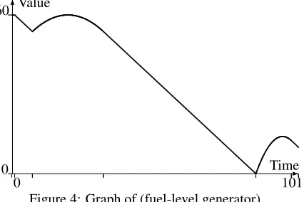
The volume of fuel of the generator for this plan is shown in figure 4.
It would be interesting to see a planner capable of pro-ducing a plan that includes the earliest or latest possible
re
-Time
6Value
0 101
0 60
Figure 4: Graph of (fuel-level generator).
fuelling, although such a plan cannot be considered very ro-bust. A better behaviour would be to push the refuelling actions comfortably into the generating interval.
4.2
Calculating a Plan Using Bounds
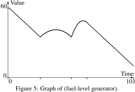
A more feasible approach to calculating a plan for a problem involving continuous effects may be to use linear approxi-mations on the continuous effects, in particular the use of step functions. For the generator problem, if we reason that a tank is only going to add 25 fuel units then we can wait un-til the generator has used up 25 fuel units, so that we know that no overflow could occur. The first refuelling would then take place at time 26. Next, the second refuelling can occur as soon as the first refuelling has finished, since we know that the volume of fuel in the generator is 35, so that no overflow could occur. Figure 5 shows the volume of fuel of the generator for this plan.
[image:4.612.336.549.320.462.2]
-Time
6Value
0 101
[image:5.612.66.282.41.189.2]0 60
Figure 5: Graph of (fuel-level generator).
51.01: (refuel generator tank2) [12.5]
Now consider what was involved in constructing this plan. The volume of fuel in the generator was calculated as a function of time from the differential equation governing its behaviour, but with no other continuous effects interacting with the volume of fuel. We then considered the refuelling action for the first tank on its own, solving the differential equation in order to figure out how long it takes to empty the tank. A step function was then used to approximate the refu-elling action, adding all of the fuel at the start of the durative action. The linear function for the generator fuel volume was then used to determine when the refuelling given by the step function could be applied. Similarly with the second tank of fuel. Notice that we did not use a step function for the generating action.
If this kind reasoning can be used to produce a plan us-ing simple calculations to handle linear functions and linear bounds for non-linear functions then this makes the plan-ning process much easier. However using linear bounds can greatly reduce the flexibility of durative actions within a plan, the more accurate continuous effects can be handled in the planning process the better the scope of valid plans that can be produced. In the generator example we saw that the earliest time a refuelling could occur using the first tank is at time 7.25. However, using linear bounds for the volume of fuel in the generator (by way of a step function on the re-fuelling action), the earliest safe time to refuel is at time 26. This reduction in flexibility might suggest that no valid plan exists at all when there are, in fact, many valid plans.
If we attempt to model the fuel-consumption of the gener-ator with a step function we have a problem: either the fuel is consumed at the start, which suggests that a tank can sim-ply transfer its 25 units of fuel to the generator at the start without exceeding the generator fuel capacity. Alternatively, if we put the consumption at the end then we cannot refuel the generator until it has ran out of fuel. In order to solve the problem we have to have access to an accurate (or at least a sufficiently accurate) model of the fuel in the generator throughout its generating time.
5
Semantics of Continuous Effects
We do not attempt to give a formal semantics in this sec-tion, due to limited space: a formal semantics has beendeveloped, based on the semantics of discrete durative ac-tions (Fox & Long 2002). The semantics of discrete durative actions can be formulated in terms of discrete state changes at the instants of change, in a familiar state-transition se-mantic framework, but with the addition of an embedding of the activity into a real time line. This is a straightfor-ward extension, except for two important complications in-troduced by the embedding: one is to explain under what circumstances the end points of actions (when instantaneous change occurs) may coincide and the other is to account for the way in which the interaction between action execution and invariants is handled. The first of these issues is re-solved by preventing action end points from coinciding if the postconditions of one of the end points include any proposi-tion that is included in the precondiproposi-tions of the other. This constraint implies that propositions are treated like shared memory in multi-processing operating systems, with actions analogous to separate processes. An action precondition de-mands read-accessto all of the atomic propositions it in-cludes, while action postconditions demandwrite-accessto all of the atomic propositions they refer to. A propositional variable can support multiple coincident read-accesses, but a write-access prevents any other access to the propositional variable. An action can, of course, refer to the same propo-sition in both its pre- and postconditions, just as single pro-cess can read and then write to a memory, because its own memory accesses are sequenced. An alternative approach, adopted by McDermott (McDermott 2003) and Bacchus and Ady (Bacchus & Ady 2001), is to allow actions that occur simultaneously to be sequenced. We consider this approach difficult to justify, since it is not clear how, in execution, simultaneous actions could actually be guaranteed to exe-cute in a specific order. A plan contains a finite number of actions. Thus, the management of invariants is handled by observing that it is only necessary to confirm each invari-ant between the finitely many discrete points of change that occur during the interval to which it applies.
Invariant Check
Invariant Check
Time
Start
Time
Start
Some Action
f
Time
0 T
End Continuous Update
End Continuous Update Invariant Check
Continuous Update 2)
1)
[image:6.612.60.288.53.239.2]3)
Figure 6: Durative action with continuous effects. Graph shows the values of a PNE,f, which is changing continu-ously during the execution of the durative action
point of change. Part (3) illustrates how discrete affects can arise, due to parallel activity during the intervals, breaking the continuous change into piece-wise continuous differen-tial components.
6
Interacting Continuous Effects
There may be a number of continuous effects active at one time each of which additively modifies the derivative of a PNE. If a PNE has its derivative modified more than once then the derivative is given by the sum of the contributions. The rate of change of a PNE may also depend on the value of other PNEs which may themselves be continuously chang-ing. The values of all the changing PNEs are thus given by a system of differential equations:dfi
dt =gi(f1, f2,· · · , fn) i∈ {1,2,· · · , n},
where the fi are the PNEs and the gi are some functions depending on the set of continuously changing PNEs. PNEs that are not changing continuously are treated as constants. For example consider the following continuous effects
increase (distance ?c) (* #t (speed ?c)) increase (speed ?c) (* #t (acceln ?c))
which describe the motion of a car driving. The rate of change of the PNE for the distance of the car is given by the PNE for the speed of the car. The PNE for the speed of the car is in turn given by the PNE for the acceleration of the car. To solve these differential equations to give the functions of time describing the motion of the car we must firstly determine the acceleration, then the speed, and lastly the distance of the car.
Solving the system of differential equations that can arise is considered in sections 8.1 and 8.2.
7
Invariants
Continuous effects have their most significant effect on the validation of plans when they interact with invariants. An in-variant condition must be evaluated on an interval by check-ing that the continuously changcheck-ing PNEs that appear within it do not assume values that lead to a violation of the invari-ant.
7.1
One-Clause Invariants
An invariant comparison containing PNEs that are contin-uously changing can always be expressed as a function of time, t, that must be greater than zero (or perhaps greater than or equal to zero. If equality is used then the difference between the left hand side and the right hand side cannot vary for the invariant to hold). For example
t2
+ 2t+ 2>0 fort∈(0,5)
may be an invariant condition to check. If the invariant ex-pression is linear in time we can simply evaluate the expres-sion at the end points of the interval to confirm the condition holds. However checking an invariant condition with a non-linear expression in time it is no longer sufficient to check the condition at end points only. An invariant comparison
F(t) >0 on(0, T), whereF is some continuous function in time,t, can be checked by one of the following methods: 1. Check thatF(0)≥0andF(T)≥0and also check that the value at any stationary points in(0, T)is greater than zero.
2. Check thatF(0)≥0andF(T)≥0and also check to see if any roots exist in(0, T). (If the inequality is non-strict then care is needed in case of repeated roots).
Method 2 is chosen to check non-linear invariants inVAL. The key to the problem of checking invariants that are com-parisons with non-linear expressions int is one of finding the roots of a non-linear function. This problem is, in gen-eral, non-trivial, even in the case of polynomials. There are many algorithms to find the roots of equations but we need to be sure of finding all the roots in a given interval in ev-ery possible case. It is therefore necessary to impose certain restrictions on the invariants that may be expressed to guar-antee that they may be verified on a given interval.
We are initially only considering invariant comparisons which depend on continuously changing PNEs that are given by polynomials int. For one-clause invariant comparisons which are given by an inequality that is strict we are in fact only interested in the existence of real roots on a given open interval. Finding the roots of polynomials is considered in section 8.3.
7.2
Invariants with Disjunctions
LetAandBbe two atoms that depend on time then consider the two conditions
A(t)∨B(t) for allt∈(0, T), (2)
(A(t) for allt∈(0, T))∨(B(t) for allt∈(0, T)). (3) It could be the case that A(t) is only satisfied on (0,3
4T] and B(t) on[1
-t
6
h2
h1
f
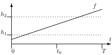
[image:7.612.82.267.56.147.2]0 t0 T
Figure 7: Example ofh1,h2 andf. Iff is required to be above h2 or below h1 across (0, T), then the value at t0 breaks the constraint.
condition (3) is not. Clearly the two interpretations are not equivalent. Suppose a durative action continuously updates a PNE,f, and there is a concurrent action (possibly the same action) with an invariant condition of the form:
f(t)< h1(t)∧f(t)> h2(t) for allt∈(0, T),
whereh1 and h2 are some functions that may depend on other functional expressions. The condition can then be checked by checking each comparison separately. However suppose the condition is of the form:
f(t)< h1(t)∨f(t)> h2(t) for allt∈(0, T),
then each comparison cannot be considered separately. In the simple case whereh1andh2 are constants andf is linear we can no longer simply check the end points of
h1−f andf −h2to be greater than zero. This is because we could have (h1−f)(0) > 0 and(f −h2)(T) > 0 which satisfies the condition at 0 and T but there could exist a pointt0 ∈ (0, T)such that(h1−f)(t0) < 0and (f−h2)(t0)<0(see figure 7).
As an example of an invariant with disjunction consider the following:
(t2
−9t+ 14≥0)∨((t−1>0)∧(−t+ 8≥0))
fortin(0,10). We must find the values oftin(0,10)each disjunct is satisfied on then take the union of the two and see if the result covers(0,10), which implies the result is in fact equal to(0,10). The first disjunct,(t2
−9t+ 14≥0), is sat-isfied for values oftin(0,2]∪[7,10). The second disjunct is not so straightforward, the condition(t−1>0)is satisfied on(1,10)and(−t+ 8≥0)is satisfied on(0,8]then taking the intersection of the two we have the disjunct being sat-isfied for values oftin(1,8]. Now taking the union of the values that the two disjuncts are satisfied on gives(0,10)
which indeed covers(0,10)showing that the invariant con-dition holds.
In general an invariant condition can be considered as a proposition in DNF that must hold over an interval, say
(0, T). To confirm the invariant, we must then find a set of intervals,C, covering(0, T), such that a disjunct is satisfied in each interval inC. This is simplified if it is possible to find all the roots of all the continuous functions involved, since these points can be used as the end points of the sub-intervals
forming the cover. In the case of polynomials this can be achieved (finding the roots of polynomials is considered in section 8.3). Even in the case of polynomials of polynomi-als, the degree of the largest polynomial is bounded giving us a tractable collection of roots and a tractable problem for validation. Using this approach means that our validation of plans cannot be more accurate than the degree of preci-sion used in the solver. However in practice, all numerical testing, even for linear functions, is subject to the degree of precision supported by our machines (always finite), so the problem of plan validation must always be qualified by an observation of the limitation on the accuracy with which nu-meric constraints can be checked.
A detail of finding a covering of(0, T)is important, let us call an exact covering of(0, T)fracturedif there is a value,
x, other than0or T, such that for everyI ∈ C ifx ∈ I
thenxis an end point ofI. (The intuition is that no interval spans between the left and right of the interval acrossx). If the only exact coverings that exist to satisfy a given invariant are fractured atxthen this implies that atxthe invariant flips from being satisfied in one way to being satisfied in another. This flip could depend on arbitrarily precise synchronisation of the activities governing the continuous change and this is unlikely to be within the power of any physical executive. For this reason, we might prefer to discount such plans as unrobust. This issue is also related to numeric precision in handling values, both in a potential executive and in the ma-chinery expected to validate a plan.
Two things (other than the form of the functions that de-scribe the behaviours of the PNEs that appear in the proposi-tion) affect the complexity of invariant checking: one is the complexity of the functions that appear in the proposition it-self and the other is whether or not there is more than one disjunct. The former is restricted to be (in ascending order of complexity) either simple linear functions, polynomials or other functions.
8
Solving Differential Equations and
Evaluating Invariants
In this section we consider approaches to solving a system of differential equations (sections 8.1 and 8.2), which arises when validating a plan with continuous effects. Then find-ing the roots of polynomials is addressed (section 8.3) as required for evaluating invariant conditions. Then finally, a general method (section 8.5) using the solutions to these problems is presented for evaluating invariants that depend on continuously changing PNEs.
8.1
Numerical Methods
of differential equations that may arise naturally in a math-ematical model. For these reasons numerical methods are very popular among scientists working with mathematical models described by differential equations. The output of numerical methods is a finite set of points which is close to the solution curve and ideally to within a given degree of accuracy. If this could be achieved then it would be sim-ple to evaluate invariant conditions by considering this set of points. Thus if we could achieve this for our system of dif-ferential equations then this would be ideal. Unfortunately a method to do this infallibly to within a degree of accu-racy for such a general system of differential equations sim-ply does not exist. The vast amount of work on the subject is a testament to this. A more realistic and desirable result would be a set of simple restrictions that could be imposed on the system of differential equations that could be easily checked whilst allowing sufficient expressibility of differen-tial equations. These restrictions could then guarantee that an efficient and infallible method could be used to obtain a solution to within a degree of accuracy (or at least the detec-tion that no soludetec-tion exists). However to the authors’ knowl-edge and disappointment no such result exists. Numerical methods are ideal if the system of differential equations is known and fixed (to within certain parameters), since then numerical methods can then be applied and guaranteed to find the an approximate solution to within a degree of ac-curacy. In our general setting we do not have this luxury so numerical methods are not appropriate, we therefore con-sider certain classes of systems of differential equations that may be solved analytically whilst allowing for sufficiently interesting planning problems.
8.2
Analytic Methods
A PNE can change as a polynomial function of time or even a more complex function of time, due to more complex de-pendencies arising in the expression on the right-hand-side of the differential equation governing its evolution. In par-ticular for a non-linear function to arise, the right-hand-side must include one or more of the PNEs that appear as left-hand-side elements (including the PNE that is governed by this equation itself).
For example consider the simple case where a PNE,f, varies with the rate of change given by:
df
dt =f
andf has a value off0 fort = 0. Then the value off is given by
f(t) =f0et.
The following proposition shows that the values taken by PNEs are given by polynomials if certain restrictions are im-posed on the differential equations.
Proposition 8.1 LetF ={f1, f2, . . . , fn}be a finite set of PNEs which are changing continuously on the interval[0, T]
given by
dfi
dt =gi(f1, f2, . . . , fn) for all i∈ {1,2, . . . , n}
where gi is some function depending onF. The function
gi is restricted to addition, subtraction, multiplication and division on its terms and division by a PNE inFis not per-mitted. If the rate of change of no PNE depends on itself (either directly or indirectly) then the value of every PNE on
[0, T]is given by a polynomial int.
Proof.Follows by induction on the dependency structure. If the conditions in Proposition 8.1 were relaxed to allow division by a functional expression then a PNE could take values given by a natural logarithm. If the dependencies could contain loops then exponential functions could occur as shown above, as well as trigonometric functions and so on.
Notice that determination of the structure of the depen-dency sets can be carried out automatically, using syntac-tic analysis of the expression parse trees. To achieve this, a graph is constructed using PNEs as vertices and with di-rected edges between the expressions on the left of contin-uous updates and those on the right of the same expression. If this graph is acyclic (which is easily tested) then the dif-ferential equations can all be solved with polynomials. The only limitation is that this dependency analysis carried out purely syntactically can be conservative, in that it might be the case that dependencies actually simplify away if ex-pressions can be symbolically manipulated to cancel terms. Since this kind of manipulation is non-trivial, we must as-sume that the dependencies discovered by syntactic analy-sis could be more restrictive than the true dependencies. It should also be observed that the dependency analysis must be considered on a case-by-case basis: each interval over which continuous change is active must be separately anal-ysed because the domain might include expressions that, in principle, allow cycles of dependency to be constructed, but no cycles might actually appear amongst effects active in the plan itself.
The complexity of the differential equations that can be expressed far exceeds the practicality of solving them and indeed the feasibility. It is therefore necessary to impose certain restrictions on the differential equations to guarantee that they can be solved.
8.3
Polynomial Root Finding
As discussed in section 7 to evaluate the truth values of in-variants it is necessary to find the roots of a polynomial on a given interval to within a given degree of accuracy. In the case of an invariant consisting of a single comparison then it is sufficient to determine only the existence or not of the roots on a given interval.
ForVALwe have chosen to implement a method based on Descartes’ Rule of Signs for several reasons: it provides an infallible solution, it is efficient, and it is relatively simple to implement. This method is subject to the polynomial con-taining no repeated roots. Fortunately for any given polyno-mial we can obtain another polynopolyno-mial with the same roots but without any repeated roots. This is achieved by divid-ing the polynomial by the greatest common divisor of it-self and its derivative. To find the greatest common divisor of two polynomials the Euclidean (a.k.a. Euclid’s or divi-sional) algorithm can be used, although the accuracy of the coefficients must be handled carefully to avoid any spuri-ous results due to rounding in the calculations. The method that we have implemented is based on Rouillier and Zimmer-mann’s algorithm (Rouillier & Zimmermann 2001), which is itself based on algorithms from Collins and Akritas (Collins & Akritas 1976).
8.4
Approximation and Power Series
On a given interval of time where there are a number of PNEs changing continuously, as defined by a system of dif-ferential equations, the PNEs may be given by arbitrary non-linear functions of time as mentioned in section 6. These non-linear functions of time may then appear in invariant conditions requiring that the functions be analysed for roots on a given interval, possibly to within a given degree of ac-curacy. It is then desirable to approximate the function in a form that can be easily used with numerical methods to compute the roots. We, of course, want to approximate the functions by polynomials, and it is a well known result that any continuous function on a closed bounded interval can be uniformly approximated on that interval by polynomials to any degree of accuracy. The most well known method of approximating continuous functions where the derivatives of all orders exist is the use of Taylor series. The Taylor series of a function can be used to obtain a polynomial approxi-mation to within a given degree of accuracy. So, given a non-linear function of time appearing in an invariant condi-tion we can find a polynomial approximacondi-tion and proceed to check the invariant using polynomial root finding tech-niques. We have used this approach inVALto handle simple exponential functions.
8.5
Plan Validation
Plan validation may be broken into segments of continuous change punctuated by a finite number of discrete changes, as discussed in section 5. These segments are given by inter-vals of time with the continuous change defined by a system of differential equations (as in proposition 8.1), F, and a set of conditions,Inv, which must hold over the interval. Each interval is considered by its local time written[0, T]. To evaluate the conditions on the given interval we use the following steps.
Step One In our answer we are assuming that we can find an analytic solution to the system of differential equations. To ensure we can find an analytic solution we impose cer-tain conditions on the system of differential equations, such as the conditions in proposition 8.1 so that the solutions are
polynomial. So for eachi= 1,· · ·, nwe havefiexpressed in terms oftwherefiis continuous on[0, T]and has deriva-tives of all orders.
Step Two For each atom in a proposition inInvwhich is a comparison depending on F such as h1(t) > h2(t) for some functionsh1andh2, we rearrange the comparison to be zero on the right hand side, h1(t)−h2(t) > 0. Then lettingg(t) = h1(t)−h2(t)we can find a polynomial ap-proximation forg to within a given degree of accuracy as mentioned in section 8.4. Thus each comparison is given by a polynomial and a boolean value to whether it is strict or non-strict. (For equality comparisons the polynomial must equal 0 and will be considered as a boolean atom for the purposes of this method).
Step Three For eachA inInvwe determine whether it holds on(0, T)as follows:
• BooleanIfAis a boolean condition then its truth value is immediate.
• ComparisonIfAis a comparison with polynomialgthen we can isolate the roots of g (if any exist). The com-parison holds on(0, T)if the end points ofgare greater than zero and no roots exist on(0, T). Evaluation ofgis needed at key points in(0, T)in the case of a non-strict comparison (in case of repeated roots) or if the end points evaluate to zero.
• ConjunctionIfAis a conjunctionA=A1∧A2∧· · ·∧Ak for somek∈ N, then we determine ifAholds on(0, T)
by checking each conjunct in order, 1tok, as given by these rules (depending on whether it is a boolean, com-parison etc.) to whether it holds for all values on(0, T). If one conjunct does not hold on(0, T)thenAdoes not hold on(0, T)and the remaining conjuncts need not be checked.
• DisjunctionIfAis a disjunctionA=A1∨A2∨ · · · ∨Ak for somek∈ N, then we determine ifAholds on(0, T)
as follows. Firstly determine the values oftin(0, T)that
A1holds on as given below, call itJ1. IfJ1= (0, T)then
Aholds on(0, T). IfJ1 6= (0, T)then we calculate the values oftthatA2holds on,J2, then ifJ1∪J2= (0, T) thenAholds on (0, T)and so on. IfSki=1Ji 6= (0, T) thenAdoes not hold on(0, T).
Values oftin(0, T)that a disjunctAiholds on:
• BooleanIfAiis a boolean value thenAiholds on(0, T) ifAiis true, otherwise it holds on the empty set.
• ComparisonIfAi is a comparison then from its corre-sponding polynomial as given in step two, we firstly find the roots in(0, T). These roots are used to determine the end points of a set of intervals that the comparison holds on. If the comparison is strict then the intervals will be open, otherwise the interval end points will be closed ex-cluding0andT.
• ConjunctionIfAiis a conjunctionAi=B1∧B2∧ · · · ∧
Bkfor somek∈N, then we determine the values oftthat
meth-ods) call itJi. TheJi’s are used to calculateTi=1···kJi, and so if there is a conjunctBj such thatTi=1···jJi =∅ then the remainingJiare not calculated.
• DisjunctionIfAiis a conjunctionAi =B1∨B2∨· · ·∨Bk for somek∈N, then we determine the values oftthatAi holds on(0, T)as follows. In order, for eachBidetermine the values oftin(0, T)it holds on (by these methods) call itJi. TheJi’s are used to calculateSi=1···kJi, and so if there is a conjunctBj such that
S
i=1···jJi= (0, T)then the remainingJiare not calculated.
For each conjunction and disjunction it is not always nec-essary to consider every conjunct or disjunct, therefore in order to save on calculation time we sort the conjuncts and disjuncts into order of estimated computational effort.
9
Conclusion
This paper examines the problem of validation of plans with continuous effects. We have implemented this approach in an extension ofVALused in the 3rd IPC (Long, Cresswell, & Howey 2003). Currently, to guarantee the validation of a plan containing durative actions with continuous effects cer-tain restrictions have to be met: all continuous effects must be given by a polynomial or a simple exponential function of time. This condition implies that the dependency graph of the rates of change of PNEs has no loops except for self dependent loops. This condition is automatically checked andVALidentifies plans that it cannot correctly validate.
In section 8 a general framework was presented to handle more complicated continuous effects; a more thorough ac-count is in preparation. Although VAL does not currently handle a wide range of types of functions, methods have been developed to do so and these methods have been imple-mented in the handling of exponential functions. The scope of the continuous functions thatVAL should handle can be seen as a prerequisite to developing planners capable of pro-ducing plans with those continuous functions. Currently, to the authors’ knowledge, the few planners handling continu-ous effects only consider linear effects. The next logical step is to develop planners capable of handling non-linear effects that are given by polynomials. This is now a much more realistic target with the availability of an automatic plan val-idation tool,VAL, capable of handling plans with polynomial effects. The extension ofVALto handle yet more complex functions at this stage would be considered overkill.
The validation of plans containing continuous effects is an important first step in making planners capable of plan-ning with languages that express them. Validation depends on semantics and cannot be implemented without removing ambiguities. The availability of a validation tool is a vital first step for the community in progressing along this path.
References
Bacchus, F., and Ady, M. 2001. Planning with resources and concurrency: A forward chaining approach. In Pro-ceedings of IJCAI’01, 417–424.
Collins, G., and Akritas, A. 1976. Polynomial real root isolation using Descartes’ rule of signs. SYMSAC.
Edelkamp, S., and Helmert, M. 2000. On the imple-mentation of Mips. In Proc. of Workshop on Decision-Theoretic Planning, AI Planning and Scheduling (AIPS), 18–25. AAAI-Press.
Fox, M., and Long, D. 2002. PDDL2.1: An extension to PDDL for expressing temporal planning domains. Techni-cal report.
Gerevini, A., and Serina, I. 2002. LPG: A planner based on local search for planning graphs. InProc. of 6th Int. Conf. on AI Planning Systems (AIPS’02). AAAI Press.
Henzinger, T. 1996. The theory of hybrid automata. In Proc. of the 11th Annual Symposium on Logic in Computer Science. Tutorial., 278–292. IEEE Computer Soc. Press. Howey, R., and Long, D. 2003.VAL’s progress: The auto-matic validation tool forPDDL2.1 used in the international planning competition. InProc. of ICAPS Workshop on the IPC.
Laborie, P., and Ghallab, M. 1995. Planning with sharable resource constraints. InProc. of 14th International Joint Conference on AI. Morgan Kaufmann.
Long, D.; Cresswell, S.; and Howey, R. 2003. Validator for PDDL2.1 plans. Available at www.cis.strath.ac.uk/∼rh/val.html.
McDermott, D., and Committee, A. I. 1998. PDDL–the planning domain definition language. Technical report, Available at:www.cs.yale.edu/homes/dvm.
McDermott, D. 2003. Reasoning about autonomous pro-cesses in an estimated-regression planner. InProc. of Int. Conf. on Automated Planning and Scheduling (ICAPS’03). Muscettola, N. 1994. HSTS: Integrating planning and scheduling. In Zweben, M., and Fox, M., eds.,Intelligent Scheduling. San Mateo, CA: Morgan Kaufmann. 169–212. Pednault, E. 1986. Formulating multiagent, dynamic-world problems in the classical planning framework. In Georgeff, M., and Lansky, A., eds.,Proc. of the Timberline Oregon Workshop on Reasoning about Actions and Plans. Penberthy, J., and Weld, D. 1994. Temporal planning with continuous change. InProc. of 12th National Conf. on AI. Rouillier, F., and Zimmermann, P. 2001. Efficient isolation of a polynomial real roots. Technical Report 4113, Rinria. Shanahan, M. 1990. Representing continuous change in the event calculus. InProceedings of ECAI’90, 598–603. Trinquart, R., and Ghallab, M. 2001. An extended func-tional representation in temporal planning: Towards con-tinuous change. InProc. of ECP-01.