Predictive Feedback Control using a Multiple Model Approach
Leonardo Giovanini and Michael Grimble
Industrial Control Centre, University of Strathclyde 50 George Street, Glasgow G1 1QE, Scotland
[email protected] [email protected]
Abstract: A new method of designing predictive controllers for SISO systems is presented. The controller selects the model used in the design of the control law from a given set of models according to a switching rule based on output prediction errors. The goal is to design, at each sample instant, a feedback control law that ensures robust stability of the closed–loop system and gives better performance for the current operating point. The overall multiple model predictive control scheme quickly identifies the closest linear model to the dynamics of the current operating point, and carries out an automatic reconfiguration of the control system to achieve a better performance. The results are
illustrated with simulations of a continuous stirred tank reactor. Copyright © 2002 IFAC
Keywords: parametric optimization, predictive control, adaptive control, robust control, feedback.
1. INTRODUCTION
Model predictive control (MPC) refers to the class of algorithms that uses a model of the system to predict the future behaviour of the controlled system and compute the control action so that a measure of performance is minimised whilst guaranteeing the fulfilment of all constraints. Predictions are handled according to the so called receding horizon optimal control philosophy: a sequence of future control actions is chosen, by predicting the future evolution of the system and these are applied to the plant until new measurements are available. Then, a new sequence is calculated so as to replace the previous one.
Schemes developed for a deterministic framework often lead to either intolerable constraint violations or over conservative control action. In order to guarantee constraint fulfilment for every possible realisation of the system within a certain set, the control action has to be chosen safe enough to cope with the effect of the worst realisation, (Gilbert and Tan, 1991). This effect may be shown by predicting the open-loop evolution of the system driven by such a worst-case system model. As pointed out by Lee and Yu (1997) this situation inevitably leads to over conservative control schemes. They suggested it is possible to exploit the control moves to mitigate the
effect of uncertainties and disturbances. This is
achieved by performing closed-loop predictions, which leads to a computationally demanding control scheme.
In the following a new predictive feedback controller
based on a Multiple Models, Switching and Tuning framework. The proposed formulation of the problem introduces feedback in the optimization of the control law, which is carried out at each sample. The multiple model approach used in this work is based on a decomposition of the system's operating range. Each operating regime of the system is modelled with a simple local linear model. Then, the closest model to the current plant dynamics is used in the algorithm to control the system.
The organisation of the paper is as follow. In section 2 the formulation of the predictive feedback control is presented. The meanings of the design parameters are discussed and the objective function is analysed from the multiobjective point of view. In Section 3 the multiple models, switching and tuning control approach is suggested by modifying the objective function and the constraints employed by the predictive feedback controller. Section 4 shows the results obtained from the application of the proposed algorithm to a nonlinear continuous stirred tank reactor. Finally, the conclusions are presented in section 5.
2. PREDICTIVE FEEDBACK
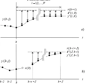
MPC is an optimal approach involving the direct use of the system model and on–line optimization technique to compute the control actions such that a measure of the closed–loop performance is minimised and all the constraints are fulfilled (Figure
1.a). The basic formulation implies a control
philosophy similar to an optimal open–loop. This can include, in a simple and efficient way, the
sinc(
i) Laboratory for Signals and Computational Intelligence (http://fich.unl.edu.ar/sinc)
k - w + J k + J
k - 2 k - 1
r(k - i + J)
ê0(J , k - i)
y0(J , k - i)
y(k - j)
k
r(k + i)
ê0(i , k)
y0(i , k)
t y(k - j)
Prediction Horizon V , , , i=12…
a)
b) u(k)
[image:2.612.116.264.38.183.2]t k
Fig. 1: MPC and Predictive Control Feedback set-ups
constraints present in the system. However, as pointed out by Lee and Yu (1997) this formulation can give poor closed-loop performance, especially when uncertainties are assumed to be time–invariant in the formulation. This is true even when the underlying system is time–invariant. When the uncertainty is allowed to vary from one time step to the next in the prediction, the open loop formulation gives robust, but cautious, control. To solve this problem, the authors suggested the exploitation of control movements to mitigate the effects of uncertainties and disturbances on the closed-loop performance. This is achieved by using the closed-loop prediction and solving a rigorous min-max optimization problem. The resultant control scheme is computationally demanding, so it can only apply to small systems with a short prediction horizon. To overcome this problem, Bemporad (1998) developed a predictive control scheme that also used closed-loop predictive action, but was limited to include a constant feedback gain.
Following the idea proposed by Bemporad (1998), Giovanini (2003) introduce a direct feedback action into the predictive controller. The resulting
controller, called predictive feedback, used only one
prediction of the process output J time intervals
ahead and a filter, such that the control movements
computed employed the last v predicted errors (see
Figure 1.b). Thus, the predictive control law given by
∑
∑= − − = + −
= w
j j v
v
j qjeˆ J,k j q u k j
k
u( ) 0 0( ) 0 ( ),
(1)
where qj j=0,1,…,v+w are the controller's
parametersand ê0(J , k - j) is the open-loop predicted
error at time k + J - j given by
,v , j j k u q , J j k e j k , J
eˆ ( ) ( ) ( ) 0,1…
1
0( − )= − −P − − ∀ = .
P (J , q-1) is the open–loop predictor given by
j N
j j
j J N
J
j j
J h q
~ q
h~ q
a ~ q ,
J = −
− + = −
− = +∑ −∑
1 1
1 1
) (
P ,
where N is the convolution length and ãJis the J–th
coefficient of the system's step response and ~hj is the
j–th coefficient of the system's impulse response. In
his work, Giovanini (2003) showed that:
• the predictive feedback controller (1) provided
better performance than a MPC controller, specially for disturbance rejection, and
• the parameters of the controller and the prediction
time, J, could be chosen independently if,
1
1 =
∑wj= qj+v .
The last fact is quite important because it makes the tuning procedure easy, since we use a stability criterion derived in the original paper (Giovanini,
2003) for choosing J and then tuning the filter using
any technique.
In this framework, the problem of handling the system’s constraints is solved tuning the parameters of the controller. This solution is not efficient because it is only valid for the operating conditions considered at the time of tuning. Therefore, any change in the operational conditions leads to a loss of optimality and violation of the constraint. The only way to guarantee the constraints fulfilment is to
optimise the control law (1) for every change that
happens in the system. Following this idea, the original predictive feedback controller is modified by including an optimization problem into the controller so that the parameters of the controller are recomputed in each sample. The structure of the resulting controller is shown in figure 2.
Remark 1 . The control action u(k), is computed
using the past prediction errors and control movements, whereas the vector of parameters –
Q(k)– is optimised over the future closed-loop
system behavior. Therefore, the resulting control law minimises the performance measure and guarantees the fulfilment of all the constraints over the prediction horizon.
After augmenting the controller, we allow the
control law (1) to vary in time
∑ ∑
= +
=
− + −
≥ ∀ − + +
= +
w j jv v
j j
j k u i k q
, i j i k , J eˆ i k q i k u
0 0
0
) ( ) (
0 ) (
) ( )
(
(2)
This fact gives us enough degrees of freedom to handle the constraints present in the system. It is well known that the optimal result is obtained when the control law is time varying. However, from experience with predictive control, many authors have pointed out that only a few control actions at time near have a strong effect on the closed-loop performance. So, we modify the control law such
that the control law is time-varying in the first U
samples and it is time invariant for the remaining samples
∑ ∑
∑ ∑
= + =
= + =
− + + +
≥ ∀ − + +
= +
− + + +
< ≤ − + +
= +
w
j jv
v
j j
w
j jv
v
j j
j i k u U k q
. U i j i k , J eˆ U k q i k u
j i k u i k q
, U i j i k , J eˆ i k q i k u
1 0
0 1
0
0
) ( ) (
) (
) ( )
(
) ( ) (
0 ) (
) ( )
( (3.a)
(3.b)
Under this design condition, in each sample a set of parameters qj(k + i) j =0 , 1 , … ,v + wi =0 , 1 , … ,U is
e(k)
-ê0(J,k)
P(J,q-1 ) C(Q(k),q-1 ) r(k)
y(k)
u(k)
Optimizer
Q(k)
y0
(J,k)
Fig. 2: Structure of the predictive feedback controller
sinc(
i) Laboratory for Signals and Computational Intelligence (http://fich.unl.edu.ar/sinc)
[image:2.612.324.507.629.729.2]computed such that the future closed-loop response would fulfil the constraints and would be optimal. Then, only the first elements of the solution vector,
qj(k) j =0 , 1 , … ,v + w, is applied and the remaining
ones are used as initial conditions for the next sample. The optimization is repeated until a criterion, based over the error and / or manipulated variable, is satisfied. When the criterion is fulfilled
the last element, qj(k +U) j =0 , 1 , … ,v + w, is
applied and the iterations stop. Usually, this criterion is selected such that the change in the control law would be produced without a bump in the closed-loop response.
Note that the design of the predictive feedback
controller (3) implies the selection of orders, the
prediction time and the parameters of the controller. In the next section we introduce the optimization problem employed to compute the parameters of the controller. In order to obtain a stabilising control law
i) the control law (3.b) must lead to an output
admissible set, called Ξ, and ii) the control law (3.b)
must be feasible everywhere in Ξ. In others word, Ξ
must be a positive invariant set (Gilbert and Tan,
1991). Therefore, this problem includes an end
constraint over the control action, called contractive
constraint, that guarantees the closed-loop stability
by selecting feasible solutions with bounded input / output trajectories.
In this framework the controller's parameters qj and
the integers v, w and J should be computed instead
of input movements u(k + i). Therefore, the control
problem is reduced to a parametric–mixed–integer optimization problem. Since this kind of problem is computational expensive, it should be changed into a
real one by fixing v, w and J.
Assuming that a set of M models W can capture a
moderate non-linearity in the neighbourhood of the nominal operating point, the parameters of the
predictive feedback control law (3) can be found
solving the following nonlinear minimisation problem
ŷ(J , k), which is used tomeasure the performance of
the system. It uses all the information available at
time k + i. The third equation is the control law (4).
Finally, the last constraint is included in this formulation to ensure closed–loop stability. It asks for null or negligible control movement at the end of the prediction horizon. Giovanini and Marchetti (1999) showed that this condition forces the exponential stability of the closed–loop system, for a step change in the setpoint. It is equivalent to
requiring both y and u remain constant after the time
instant k+V. It therefore ensures the internal stability
of all open–loop stable system. It also helps to select feasible solutions with bounded input / output trajectories and consequently it speeds up the numerical convergence. Furthermore, it avoids oscillations and ripples between sampling points.
The tuning problem (4) consists of a set of constraints
for each model of the set W, with control actions
u(k-j) j=1,…,w and past errors e(k - j) j=1,…,v as
common initial conditions and the parameters of the controller as common variables. The tuning problem
readjusts the predictive feedback controller (4) until
all the design conditions are simultaneously satisfied, by a numerical search through a sequence of dynamic simulations. The key element of this controller is to find a control law implicitly satisfying the terminal condition. This reduces the computational burden in the minimization of the performance measure. Furthermore it replaces the open–loop prediction by a stable closed–loop prediction thereby avoiding the ill–conditioning problems.
Figure 2 reveals the structure of the resulting predictive controller. Observe that the actual control
action u(k), is computed from the past predicted
errors and control movements, whereas the vector
parameters Q(k) is optimised over the future closed–
loop system behaviour. The resulting vector minimises the performance measure and guarantees the fulfilment of all constraints over the prediction
horizon V.
ε ≤ ∆
∈ − + + +
− + +
=
− ∈ − + + +
− + +
=
∈ +
+ +
=
∈ +
= +
+
∑ ∑
∑ ∑
∑
= + =
= + =
=
) (
] [ ) ( ) ( )
( ) ( )
(
] 1 0 [ ) ( ) ( )
( ) ( )
(
], [1 )
( )
( ) ( ) ( ) (
], 0 [ )
( ) ( ) ( ) (
)) ( ) ( ) ( (
1 0
0
1 0
0
0 1
1 0
V u
V , U i j i k u U k q j i k , J eˆ U k q k , i u
U , i j i k u i k q j i k , J eˆ i k q k , i u
M , l j
k u h ~ k u J,q k y k , i y ˆ
V , i k
, i u J,q k y i k , J y ˆ
st.
k , i u , k , i y , i k r F min
l
w
j jv l
v
j j l
w
j jv l
v
j j l
i
j jl l
-l l
-l
l
l l k
P P
(4)
where V is the overall number of samples instants
considered, l ∈[1 , M] stands for a vertex model and
M is the number of models being considered.
The objective function F( : ) in (4) is a measure of the
future closed–loop performance of the system. It considers all the models used to represent the controlled system. The first constraint is the
corrected open–loop prediction ^ŷ0(J , k) which is
employed to compute the control action u(i , k). It
only uses the information available until time k + i.
The second constraint is the closed–loop prediction
In control scenarios, it is natural that inputs and outputs have limits (such us actuator rate limits). The particular numerical issues discussed in this paper are the same whether such constraints are included or not.
2.1. The objective function
Notice that the polytope W that must be shaped
along the prediction horizon V. Hence, the objective
function should consider all the linear models in simultaneous form. At this point, there is no clear
sinc(
i) Laboratory for Signals and Computational Intelligence (http://fich.unl.edu.ar/sinc)
information about which model is the appropriate one to represent the system. A simple way of solving this problem is using a general index
∑=
= M l lfl
F(:) 1γ (:), (5)
where γl≥0 are arbitrary weights and fl is the
performance index for model l measured by any
weighting norm
∞ ≤ ≤ =
+
= eˆi,k Ru i,k i , ,V, p :
fl() ( ) p ( ) p 0… 1 .
The coefficients γl allow us to assign a different
weight to each index corresponding to model l,
emphasising or not the influence of a certain model in the control law.
In general, the solution obtained by the problem (4),
with objective function given by (5), produces a
decrease in someone of the components of F, say
fn n∈[1,M], and the increase of the remaining, fm
m≠n, m∈[1,M]. The minimisation of the general
index F depends on the effect of each one of the
component fl over the index. Thus, the best solution
doesn’t necessarily coincide with one of the optimal singular values. It is necessary a trade off among the
different components of the general index F.
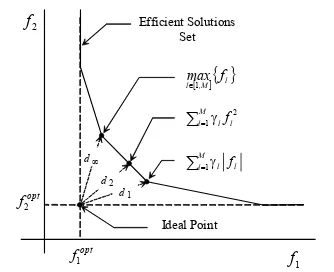
The problem (4) with the objective function (5),
corresponds to a hybrid characterization of the
multiobjective problem (Chankong and Aimes, 1983), where the performance is measured through a
weighted-norm objective function (5) and the design
constraints are considered through the additional restrictions. In this framework, the performance
index (5) can be seen as the distance between the
ideal solution, which results from the minimum of each component, and the real solution (Figure 3). So,
the solutions given by the problem (4) would
minimise the distance between the ideal and the feasible solutions, approaching them as closely as the design constraints and the system dynamics will allow.
Remark 2. If only one of the weights is not null, said
γm m∈[ 1 ,M], the resulting control law will obtain
the best possible performance for the selected model and will guarantee the closed-loop stability for the remaining models.
In this case, the closed-loop performance achieved
by the model m will be constrained by stability
requirements of the remaining models. Therefore, it is possible that the performance obtained by the
model m differs from the optimal singular value.
This formulation of the optimization problem enjoys an interesting property that is summarised in the following theorem:
Theorem 1. Given the optimization problem (4) with
the objective function (5), the norm employed to
measure the performance is different to the worst
case (p≠∝) and γl>0 l =1 ,…,M, then any feasible
solution is at least a local non-inferior solution.
Proof: See Theorems 4.14, 4.15 and 4.16 of
Chankong and Aimes (1983).
The main implication of this theorem is the fact that
any feasible solution provided by the problem (4)
with the objective function (5) will be the best
possible and it will provide an equal or a better
Efficient Solutions Set
f1
fopt
2
fopt
1
[ ]{ }l M ,
l f
max
1
∈
Ideal Point
f2
∑=γ
M
l1 lfl
2
∑=γ
M l1 l fl
d1 d2 d∞
Fig. 3: Solutions sets in the controller objective space for several measures of performance for M=2.
closed-loop performance than the worst case model formulations of predictive controllers.
3. MULTIPLE MODELS, SWITCHING and
TUNING CONTROL
In almost all-industrial applications the design of a controller assumes that the plant is approximately linear. In practice this is too strong a simplification. The resulting controller often leads to either intolerable constraint violations or over conservative control action. In order to guarantee constraint fulfilment for every possible realisation of the system
within a certain set W , it is enough to cope with the
effect of the worst realisation (Gilbert and Tan, 1991).
To get a good performance on a wider-constrained operating range, it is necessary to use the closest
model of W to the current plant dynamic. This idea
implies the use of Multiple Model, Switching and Tuning Control (MMST) schemes (Goodwin et al., 2001). It is based on the idea of describing the dynamics of the system using different models for different operating regimes, and to devise a suitable strategy for finding the model that is closest (in some sense) to the current plant dynamics (Figure 4). This model is used to generate the control actions that achieve the desired control objective. The main feature of this approach is that for linear time invariant systems, under relatively mild conditions, it results in a stable overall system in which asymptotic convergence of the output error to zero is guaranteed (Frommer et al., 1998).
Generally, the switching algorithm is implemented by first computing the performance indices
] 1 [ ) ( )
( )
( 0 0 2
2 2
1e k c e k l ,M
c k
I kik l
k i l
l = + ∑= ρ ∈
−
(6)
where c1>0, c2>0 , ρ∈[0,1], k0 is the sampling
when the change happens and
,M , , l k y k y k
el( )= ˆl( )− ( ) =12…
The scheme is now implemented by calculating and comparing the above indices every sampling instant,
generating the switching variables Sl(k) from
( )
−
=
∈min ( ) ( )
) (
] , 1 [
k I k I H k
S l l
M l
l , (7)
where H(x) is the Heaviside unit step function given by
< ≥ =
. 0 0
, 0 1 ) (
x x x
H (8)
sinc(
i) Laboratory for Signals and Computational Intelligence (http://fich.unl.edu.ar/sinc)
[image:4.612.335.502.32.168.2]Gp1(z) Gp2(z) Gp3(z) Gp4(z)
GpM(z) GpM-1(z)
I2(k)
I1(k) I3(k)
IM(k ) IM-1(k)
I4(k) Current plant
dynamic
[image:5.612.316.513.30.173.2]System Operating region Fig. 4: Geometrical interpretation of index (7).
The objective function (5) - employed in problem
(3)- is modified by replacing the weight γl by the
switching variables Sl(k), which are computed
outside the controller, for each model by including them in the design constrains. The objective function
(4) and the design constraints are given by
(
)
(
)
(
S ku k i,k)
,g
, k , i k y k S g
, V , , i i k u i k y i k r f k S : F
l l u
l l y M l
0 ) ( ) (
0 ) ( ) (
1 ) ( ), ( ), ( ) ( )
( 1
≤ +
≤ +
= + + +
=∑= … (9)
(10)
Let us observe that the predictive feedback controller
(3) is designed, by problem (4) with objective
function (9) and constraints (10), only employing the
closest model to the current plant dynamic, which is used to measure the performance and evaluate the constraints. Then, a better closed–loop performance is obtained because a less conservative model is used to design the controller. However, note that the stability of the nonlinear system is guaranteed because the predictive feedback controller satisfies
the stability condition for all model of W. Thus, the
resulting control law will stabilise the system in the whole-operating region and will obtain the best performance for the current operating point.
The structure of the predictive feedback controller must be modified by including the switching
variables Sl(k) as external inputs of the optimiser.
4. SIMULATION AND RESULTS
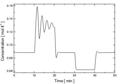
Now, let us consider the problem of controlling a continuous stirred tank reactor (CSTR) in which an irreversible exothermic reaction is carried out at constant volume. This is a nonlinear system previously used by Giovanini (1993) to test discrete control algorithms. Figure 5 shows the dynamic responses to the following sequence of changes in
the manipulated variable qC+10 lt min
-1
, -10 lt min-1,
-10 lt min-1 and +10 lt min-1, where the nonlinear
nature of the system is apparent.
Four discrete linear models were determined using subspace identification technique (Van Oversheet and De Moore, 1995) to adjust the composition responses to the above four step changes in the manipulated variable (Table 1). Notice that those changes imply three different operating points
corresponding to the following stationary
manipulated flow-rates: 100 lt min-1, 110 lt min-1
and 90 lt min-1. They define the polytope operating
region being considered and it should be associated
to the M vertex models in the above problem
formulation (4) with objective function (9).
0 10 20 30 40 50
0.06 0.08 0.10 0.12 0.14 0.16
C
o
n
c
e
n
tr
a
ti
o
n
[
m
o
l
lt
-1 ]
Time [ min ]
Fig. 5: Open loop responses of the CSTR concentration.
Like in the previous work, the sampling time period
was fixed in 0.1 min., which gives about four
sampled-data points in the dominant time constant when the reactor is operating in the high concentration region. The open–loop predictor of the
controller, P(J , q-1), and the open–loop predictors of
optimization problem, Pl(J , q
-1
) l =1 , 2 , 3 , 4 , are
built using a convolutional model of 200 terms. It is
obtained from the model 1 (Table1), because the CSTR is more sensitive in this operation region.
Finally, the parameters v and w were adopted such
the resulting controller the resulting controllers
include the predictive version of popular PI
controller (v =2 and w=1), the prediction time J was
fixed such that it guarantee the closed-loop stability,
J =9 (Giovanini, 2003) and U=7.
In this application we stress the fact that the reactor
operation becomes uncontrollable once the
manipulated exceeds 113 lt min-1. Hence, assuming a
hard constraint was physically used on the coolant
flow rate at 110 lt min-1, an additional restriction for
the more sensitive model (Model 1 in Table 1) must
be considered for the deviation variable u(k),
k k
u1( )≤10 ∀ . (11)
In addition, a zero–offset steady–state response and a
settling time of 5 min are demanded (the error must
be lower than 10-3 mol lt-1). Thus we include the
following constraints
, N k k
e
, k k
r . k y
O 50
10 ) (
) ( 03 1 ) (
3 ∀ ≥ +
− ≤
∀
≤ (12.a)
(12.b)
where NO is the time instant when the setpoint
change happens. This assumes that the nominal
absolute value for the manipulated is around 100
lt min-1 and that the operation is kept inside the
polytope whose vertices are defined by the linear
[image:5.612.101.288.39.162.2]models. Constraints (11) and (12) are then included
Table 1 Vertices of the Polytope Model
Step Change Model Obtained
Model 1
QC = 100, ∆qC = 10
9406 0 8935 1
10 1859 0
2
5 3
. z . z
z .
+ −
− −
Model 2
QC= 110, ∆qC = -10
7793 0 7272 1
10 2156 0
2
5 3
. z . z
z .
+ −
− −
Model 3
qC= 100, ∆qC = -10
7547 0 7104 1
10 1153 0
2
5 3
. z . z
z .
+ −
− −
Model 4
QC= 90, ∆qC = 10
8241 0 7922 1
10 8305 0
2
5 4
. z . z
z .
+ −
− −
sinc(
i) Laboratory for Signals and Computational Intelligence (http://fich.unl.edu.ar/sinc)
[image:5.612.316.517.618.744.2]in (4). Furthermore, the objective function adopted for each model in this example is the same used by Giovanini (2003)
∑= + +λ∆ +
= V
l
l : eˆk i u k i
f i0
2
) ( ) ( )
( (13)
where the time span is defined by V = 200.
To analyse the effect of a switching scheme on the closed–loop performance a predictive feedback
controller without the MMST scheme was
developed. The only differences between them are
the parameters v and w. They were fixed to v = 4 and
w= 4, such that the closed-loop poles could be
arbitrarily located.
Giovanini and Marchetti (1999) previously used with this reactor model for testing different predictive controllers and confronted the results with the
responses obtained using a PI controller. The
parameters of the PI parameters were adjusted by the
ITAE criterion; thus we used the same settings: the
gain value, 52 lt2mol-1min-1 and the integration time
constant, 0,46 min. The simulation tests consist of a
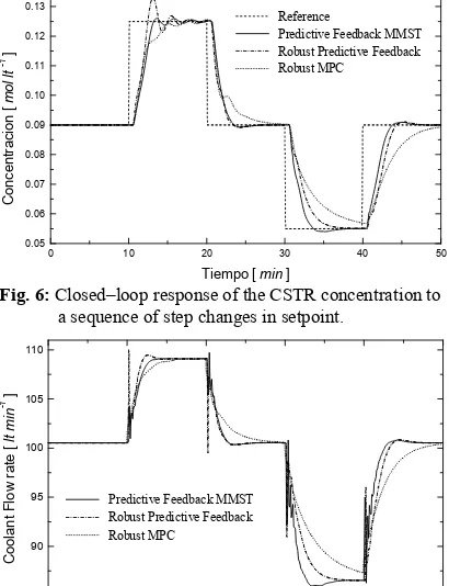
sequence of step changes in the reference value. Figure 6 shows the results obtained when comparing both predictive controllers for same changes in the setpoint. The controller with MMST scheme gives a superior performance. The improvement of the closed–loop performance is obtained through better exploitation of manipulated constraint (Figure 7), due to the retuning of the control law. For those regions with similar behavior (Models 2, 3 and 4),
the proposed controller provides symmetric
responses and satisfied constraints (11) and (12),
despite of the uncertainties.
As was anticipated, the predictive controller without MMST showed a poorer performance. It only failed
0 10 20 30 40 50
0.05 0.06 0.07 0.08 0.09 0.10 0.11 0.12 0.13
Reference
Predictive Feedback MMST Robust Predictive Feedback Robust MPC
C
o
n
c
e
n
tr
a
c
io
n
[
m
o
l
lt
-1 ]
[image:6.612.94.299.430.697.2]Tiempo [ min ]
Fig. 6: Closed–loop response of the CSTR concentration to a sequence of step changes in setpoint.
0 10 20 30 40 50
85 90 95 100 105 110
Predictive Feedback MMST Robust Predictive Feedback Robust MPC
C
o
o
la
n
t
F
lo
w
r
a
te
[
lt
m
in
-1 ]
Time [ min ]
Fig. 7: Manipulated movements corresponding to the responses in Fig. 6.
to fulfil the amplitude constraint (12.a) (see Figure 6).
This predictive controller needed to violate this constraint in order to fulfil the remained ones. For those regions with similar behavior (Models 2, 3 and 4), this controller also provided symmetric responses.
5. CONCLUSIONS
A simple framework for the design of a robust predictive feedback controller with multiple models was presented. The approach was to relate control law performance to the prediction of performance. The resulting controller identifies, at each sample, the closest linear model to the actual operational point of the controlled system, and reconfigures the control law such that it ensures robust stability of the closed–loop system. The reconfiguration of the controller is carried out by switching the function used to measure the closed–loop performance and the constraints.
The results obtained by simulating a continuously stirred tank reactor with significant non-linearities show the effectiveness of the proposed controller.
Acknowledgements: We are grateful for the financial
support for this work provided by the Engineering and Physical Science Research Council (EPSRC) grant Industrial Non-linear Control and Applications GR/R04683/01.
REFERENCES
Bemporad, A. (1998). “Reducing conservativeness in predictive control of constrained system with
disturbances”, in Proc. IEEE Conference on
Decision and Control, pp.2133–2138.
Chankong, V. and Y. Haimes (1983). Multiobjective
Decision Making: Theory and Methodology,
Elsevier Science Publishing Co., New Holland, New York.
Frommer, J., S. Kulkarni, and P. Ramadge (1998).
“Controller Switching Based on Output
Prediction Errors“, IEEE Trans on Autom.
Control, vol. 43(5), pp. 596 –607.
Gilbert, E and K. Tan (1991). “Linear Systems with State and Control Constrains: The Theory and Application of Maximal Admissible Output
Sets”, IEEE Trans on Autom. Control, vol. 42(3),
pp. 1008 – 1020.
Giovanini, L. and J. Marchetti (1999). “Shaping
Time-Domain Response with Discrete
Controllers”, Ind. Eng. Chem. Res. vol. 38(12),
pp. 4777 – 4789.
Giovanini, L. (2003). “Predictive Feedback Control”,
ISA Transaction Journal, vol. (2), pp. 206–227.
Goodwin G., S. Graebe and M. Salgado (2001).
Control System Design, Prentice Hall: Englewood
Cliffs, New York.
Lee, J and Z. Yu (1997). “Worst-case Formulation of Model Predictive Control for System with
Bounded Parameters”, Automatica, vol. 33(5), pp.
763 – 781.
Van Overschee P. and B. De Moor (1996). Subspace
Identification for Linear System. Kluwer
Academic Publisher.
sinc(
i) Laboratory for Signals and Computational Intelligence (http://fich.unl.edu.ar/sinc)