Using frequency detuning to compare analytical approximations for forced responses

approximations for forced responses

.

White Rose Research Online URL for this paper:

http://eprints.whiterose.ac.uk/151031/

Version: Published Version

Article:

Elliott, A.J., Cammarano, A., Neild, S.A. et al. (2 more authors) (2019) Using frequency

detuning to compare analytical approximations for forced responses. Nonlinear Dynamics.

ISSN 0924-090X

https://doi.org/10.1007/s11071-019-05229-6

[email protected] https://eprints.whiterose.ac.uk/ Reuse

This article is distributed under the terms of the Creative Commons Attribution (CC BY) licence. This licence allows you to distribute, remix, tweak, and build upon the work, even commercially, as long as you credit the authors for the original work. More information and the full terms of the licence here:

https://creativecommons.org/licenses/

Takedown

If you consider content in White Rose Research Online to be in breach of UK law, please notify us by

https://doi.org/10.1007/s11071-019-05229-6

O R I G I NA L PA P E R

Using frequency detuning to compare analytical

approximations for forced responses

A. J. Elliott _· A. Cammarano _· S. A. Neild _· T. L. Hill · D. J. Wagg

Received: 17 December 2018 / Accepted: 16 August 2019 © The Author(s) 2019

Abstract It is possible to use numerical techniques to provide solutions to nonlinear dynamical systems that can be considered exact up to numerical tolerances. However, often, this does not provide the user with suf-ficient information to fully understand the behaviour of these systems. To address this issue, it is com-mon practice to find an approximate solution using an analytical method, which can be used to develop a more thorough appreciation of how the parameters of a system influence its response. This paper considers three such techniques—the harmonic balance, multiple scales, and direct normal form methods—in their abil-ity to accurately capture the forced response of nonlin-ear structures. Using frequency detuning as a method of comparison, it is shown that it is possible for all three methods to give identical solutions, should particular conditions be used.

Keywords Nonlinear·Vibration·Normal form·

Multiple scales

A. J. Elliott (

B

School of Engineering, University of Glasgow, Glasgow G12 8QQ, UK

e-mail: [email protected]

S. A. Neild·T. L. Hill

Department of Mechanical Engineering, University of Bristol, Bristol BS8 1TR, UK

D. J. Wagg

Department of Mechanical Engineering, University of Sheffield, Sheffield S1 3JD, UK

1 Introduction

contin-uation can greatly increase for larger systems, which limits this numerical strategy to low-order applications. In this work, the accuracy of three analytical meth-ods in capturing the behaviour of a nonlinear system is assessed. Namely, these are the harmonic balance (HB), the multiple scales (MS), and direct normal form (DNF) techniques. These methods were chosen due to their wide application in the literature and, therefore, the results provide the user with the make a more informed decision regarding the accuracy and applicability of the methods. It should be noted that these techniques do not represent the entire field of analytical meth-ods for approximating nonlinear systems; for example, the more mathematically rigorous spectral manifolds approach may also be applied (see [12]) A more com-plete review of the associated literature is presented in [3]. However, as motivation for their comparison, we present some prominent studies including each of the considered techniques. The HB balance method has been widely used to identify nonlinearities in mechani-cal structures [13–15], as well as calculating their non-linear normal modes [16]. Furthermore, in [17], it has been shown that the relative simplicity of the method permits the use of large number of harmonics, allow-ing the accurate prediction of the behaviour of complex structures. There are a number of ways in which the MS method can be applied, as has been discussed in [18]. It has been widely used in the prediction of non-linear dynamic behaviour, such as bifurcations in the frequency–amplitude relationship [19–22] and internal resonances [23–25]. These resonances have also been investigated using the DNF method [26–29], which has been further applied to explore the significance of non-linear normal modes in relation to forced cases [30] and identify nonlinearity in structures [31,32].

This paper expands the recent discussion by the authors in [3], which considered the calculation of the free response of two nonlinear mass-spring sys-tems using the MS and DNF techniques. The authors applied the frequency detuning from the DNF method, as explored in [33,34], in the MS technique to show that it is possible for both methods to give identical solu-tions. In the current study, this discussion is expanded in a number of ways, though the desire to achieve accu-rate results with minimal analytical effort remains a priority. First, the widely applied harmonic balance (HB) method is included in the discussion, providing a more exhaustive assessment of analytical approxima-tion methods. Furthermore, the three methods are now

applied to forced, damped systems, allowing the valid-ity and applicabilvalid-ity of the discussion to be expanded to situations which more closely represent real-world engineering applications. Finally, the variable nature in which the MS method can be applied is addressed by using the derivative expansion version [35,36], as opposed to the two-timing variant [1,37].

This paper is structured as follows: Sect.2provides an overview of the analytical techniques considered; these methods are then applied to a Duffing oscillator in Sect.3; frequency detuning is used to compare the methods in Sect.4; graphical results are presented in Sect.5; and conclusions are drawn in Sect.6.

2 Overview of techniques

In this paper, the techniques are initially presented with reference to a nonlinear, dynamical system, in which it is assumed that the damping, forcing, and nonlin-ear terms produce relatively small contributions to the system behaviour. The equations of motion of such a system are defined by

Mx¨+(ε)Cx˙+Kx+(ε)Ŵx(x,r)=(ε)Pxr, (1)

whereM,C, andKdefine the linearN×Nmass, damp-ing, and stiffness matrices, respectively,Ŵxis anN×1 vector of the nonlinear terms, and the dot notation rep-resents derivatives with respect to time,t. In addition, rT= [rp,rm] = [e+jΩt,e−jΩt]represents the periodic

nature of the forcing applied andPx=

_ˆ

Px

2,

ˆ

Px

2

, where

ˆ

Pxis anN×1 vector of scalar terms which define the magnitude of this forcing. The bookkeeping parame-ter,ε—used to denote the relatively small nature of the damping, nonlinear, and forcing terms—is bracketed to denote the fact that it is not necessarily used in the HB method.

Applying the modal transformation and pre-multiplying the resultant equation byTgives (TM)q¨+(ε)(TC)q˙+(TK)q

+(ε)TŴx(q,r)=(ε)TPxr. (2) Therefore, by pre-multiplying Eq. (2) by(TM)−1, the modal equations of motion can be simplified as

¨

q+q+(ε)Ŵq(q,q,˙ r)=(ε)Pqr, (3)

whereqis anN×1 vector of modal contributions,=

(−1M−1K) is a diagonal matrix of squared fre-quency terms,ω2_n,i, andPq=−1M−1Pxis the modal projection of the forcing amplitudes. Ŵq(q,q,˙ r) = (−1M−1C)q˙ +−1M−1Ŵx(q,r)is a function that contains the nonlinear terms, similarly to Ŵx in Eq. (1), but is here expanded to include damping terms.

2.1 Harmonic balance method

Widely used across the literature [13–17,38,39], the HB method begins with the assumption that the ith displacement,qi, can be expressed in the form

qi(t)= n

k=1

Ak,i 2 e

+j(kωrt+φi)₊ A¯k,i 2 e

−j(kωrt+φi)_{, (4)}

wheren denotes the number of harmonic terms to be included in the trial solution, Ai and φi define the ith amplitude and phase, respectively, and the nota-tion¯•represents the complex conjugate.ωrdenotes the response frequency; note that this is the true frequency at which the system will oscillate, and this may dif-fer from the forcing frequency,Ω. Thus, this assump-tion states that the time-varying displacement can be expressed as a series of harmonic terms which contain frequency content at integer multiples ofωr,i.

The displacement expression defined in Eq. (4) can be applied in Eq. (2) to give a system of polynomials in terms of e+jΩt, effectively collecting the terms that respond at each frequency. The terms of these polyno-mial equations are then functions ofAi andφi. Since these equations are time-dependent, the coefficients of the harmonic terms must be balanced, as suggested by the name of this method. In fact, this balancing of har-monic terms is an integral step of both the MS and DNF methods, as both require the assumption that the coefficients of like harmonic terms must be equal.

2.2 Multiple scales technique

As previously mentioned, the derivative expansion ver-sion of the MS is used in this paper [1,37]. This version begins by first perturbing the time and displacement as

t =T0+T1+T2· · · =t+εt+ε2t+ · · · ,

q=q₀(T0,T1,T2, . . .)+εq1(T0,T1,T2, . . .)

+ε2q₂(T0,T1,T2, . . .)+. . . , (5)

respectively. From the latter of these, it is possible to define the derivatives with respect to time,t, as

d

dt =D0+εD1+ε

2_D

2+ · · · ,

d2 dt2 =D

2

0+ε(2D0D1)+ε2(D12+2D0D2)+ · · · ,

(6)

where Dn denotes the derivative with respect to Tn. Implementing these definitions in Eq. (3) leads to the equation

((D₀2+ε(2D0D1)+ε2(D21+2D0D2)+ · · ·)+)

(q₀+εq₁+ε2q₂+ · · ·)

+εŴq(q0+εq1+ε2q2+ · · ·,

(D0+εD1+ε2D2+ · · ·)

(q₀+εq₁+ε2q₂+ · · ·),r)=εPqr, (7)

This step is explored further in [40]. To resolve the complexŴqterm, it is useful to apply a Taylor expan-sion, so that the balanced exponents of Eq. (7) can be written as

ε0:(D2₀+)q₀=0,

ε1:(D2₀+)q₁= −2D0D1q0

−Ŵq

q₀, d dt(q0),r

+Pqr,

ε2:(D2₀+)q₂= −2D0D1q1−(D21+2D0D2)q2

−

_∂

∂q₀Ŵq

q₁−

_∂

∂q˙₀Ŵq

˙

q₁,

..

. (8)

where

∂ ∂q₀Ŵq

denotes the vector of partial derivatives

ofŴqwith respect to each of the elements ofq0.

q0,i = Ai

2 e

+j(ωr,iT0+φi)_{+c.c., (9)}

whereAiandφidenote theith displacement and phase components, as they were in the HB method. However, unlike the previous technique, both of these parameters are now dependent on the faster timescales,T1,T2, . . ..

Once this solution has been established, it can be implemented in the ε1-order equation. In doing so, it must be noted that the homogeneous form of this expression is identical to that used to findq₀. Therefore, those terms which respond atωr,i—referred to as secu-larterms—must be set to zero. The reason for doing so is that the homogeneous forms of theε0- andε1-order expressions are the same, so these secular terms would lead to a divergent solution in the latter; further details are given in “Appendix A”. The solution of this expres-sion leads to the frequency–amplitude relationship.

Then, only the non-secular terms are used to find a solution forq₁by considering the updated expression

(D₀2+)q₁= −NResŴq

q₀, d dt(q0),r

. (10)

where NRes{•}denotes the non-resonant component of•.

This process can then be repeated to find higher-order displacement expressions.

2.3 Direct normal form technique

Having applied the modal transform to the equations of motion in Eq. (3), two further transforms are applied as part of the DNF method; these can be summarised as [1,33]:

– Forcing transform

– The terms in the response which respond at fre-quencies close to the forcing frequency are iso-lated.

– Nonlinear near-identity transform

– This transform is used to remove those nonlin-ear terms which are non-resonant.

The forcing transform takes the formq = v+ [e]r, where v is the transformed state of q and [e] is an

N×2 matrix used to isolate the resonant forcing terms, an explicit definition of which is given subsequently.

Applying this transform in the modal equations of motion gives

¨

v+ [e]WWr+v+[e]r

+εŴv(v+ [e]r,v˙+ [e]Wr,r)=Pqr, (11) whereWis a 2×2 diagonal matrix with entries+jΩ and−jΩ.andrare defined as in the previous sec-tion. This step is used to monitor which terms are close to resonance, which, for thekth mode, will be taken to mean ωn,i ≈ Ω. Thus, thekth row of Pv can be explicitly written as

Pv,k =

Pq,k if ωn,i ≈Ω,

[0 0] otherwise. (12)

It is desirable to write Eq. (11) in the form

¨

v+v+εŴv(v,v,˙ r)=εPvr, (13)

where any non-resonant forcing terms have been removed. This can be achieved by imposing the def-initions

Ŵv(v,v,˙ r)=Ŵq(v+ [e]r,v˙+ [e]Wr,r) and Pv=Pq+[e] − [e]WW. (14) Applying the definition ofW, theith row in the latter of these definitions can be expressed as

Pq,i =Pv,i +(ω2n,i−Ω2)[e]i. (15)

Combining this expression and Eq. (12), it is possible to explicitly define thekth row of[e]as

[e]k=

[0 0] if ωn,i ≈Ω, Pq,k/(ω2n,i −Ω2) otherwise.

(16)

Now, the nonlinear near-identity transform is applied, allowing the response to be separated into its fun-damental (u) and harmonic (h) components. This is achieved by implementing the following expression for v:

v=u+εh(u,u,˙ r), where h(u,u,˙ r)=h1(u,u,˙ r)

+εh2(u,u,˙ r)+ · · · . (17)

it is assumed that the expression foru is sinusoidal and will be written in exponential form, with separate vectors for the positive and negative exponents; this is expressed asu=up+um, where the subscripts denote the sign of the exponent. Therefore, theith element of uis now written as

ui =upi +umi = Ai

2 e

+j(ωr,it+φi)₊ Ai 2 e

−j(ωr,it+φi)_,

(18)

whereAi,φi, andωr,idenote the amplitude, phase, and response frequency ofui, respectively.

As in Eq. (13), the desired form for the equations of motion in this step, with the non-resonant nonlinear terms removed, is given by

¨

u+u+εŴu(u,u,˙ r)=Pur. (19)

Following the procedure defined by [1], it is possible to implement Eq. (17) in Eq. (13), and then apply Eq. (19) to give the simplified,ε1-order expression

(εh¨1+ε2h¨2+ · · ·)+(εϒh1+ε2ϒh2+ · · ·)+εŴv −(εŴu,1+ε2Ŵu,2+ · · ·)+Pur−Pvr=0. (20) This equation applies the perturbationŴu(u,u,˙ r) =

Ŵu,1(u,u,˙ r)+εŴu,2(u,u,˙ r)+ · · · and notes that

¨

u= ϒu, whereϒis a diagonal matrix withith term ω_r2_,i. Furthermore, the following detuning expression has been employed:

=ϒ+ε=ϒ+ε(−ϒ), (21)

a step which is typically applied in the DNF method and is explored further in [33,34]. The first equality here demonstrates the fact that instead of simply detun-ing around the natural frequency, we detune its square, as this is the form in which it arises in the equations of motion. The second expression makes use of the fact that althoughis not necessarily equal toϒ, the dynamics are considered within some close neighbour-hood of the natural frequency, so their difference will be small (and hence of orderε).

Balancing theε0terms in Eq. (20), it can be seen thatPu =Pv. In theε1-order balance, theŴu,i terms are used to manage resonant terms, which respond at ωr,i. These expressions typically comprise polynomi-als in terms ofup = {upi},um = {umi}, andr. The procedure for deriving the fundamental and harmonic

responses from these polynomials is more thoroughly outlined in “Appendix B”, but is briefly outlined here. In the DNF method, and in contrast with the other methods discussed in this paper, the matrix notation u∗_i(up,um,r)is introduced. This expression is simply anNi×1 vector including all the possible polynomial terms which could arise in the aforementioned expan-sion ofŴu,i. This vector can then be pre-multiplied by a matrix of time-independent coefficients for each entry inu∗_i; a more detailed explanation of this is given in “Appendix B”.

Then, the difference between the frequency of these entries and the response frequency is captured by the introduction of the matrix β_i, with element {k, ℓ}

defined by

βi,k,ℓ= [ω∗i,ℓ]2−ω2r,i. (22)

This is done so that it is possible to easily isolate the fun-damental and harmonic components of the response, which are captured by the coefficient matrices[Γu,i] and[h], respectively. Effectively, β_i is used here to separate the resonant and non-resonant terms of[Γv,i]. Once this has been done, it is possible to express the frequency–amplitude relationship as

(ω_n2_,i−ω_r2_,i)Uie−jφi +Γui+=Pui, (23)

as derived in “Appendix B”.

As well as finding this relationship, it is possible to calculate the harmonic response using Eq. (17), so that the physical response of the general nonlinear system is

q=u+εh(u,u, εr)˙ +ε[e]r. (24)

3 Application to a Duffing oscillator

This section focuses on the application of these ana-lytical approximation methods to the single-degree-of-freedom (SDOF) Duffing oscillator, with equations of motion

¨

x+2(ε)ζ ωnx˙+ω2nx+(ε)αx

3_=(ε)P

cos(Ωt). (25)

an example application of the discussion above that is easily accessible to the reader; this could be expanded to include more complex structures in future works, though the conclusions drawn would be similar to those in this paper. Given there is only one DOF, the system is automatically written in modal coordinates, allowing a cosmetic change to give

¨

q+2(ε)ζ ωnq˙+ω2nq+(ε)αq3=(ε)Pcos(Ωt). (26)

As such, it is possible to directly follow the modal appli-cation of the analytical techniques, as defined in Sect.2. In this comparison, the solutions will be found up to ε1-order. Theε2-order solutions are qualitatively sim-ilar to those shown in this section, but are more alge-braically complicated and, therefore, are not presented.

3.1 Harmonic balance method

In this example, across all three methods, it will be assumed that only a single harmonic term will be nec-essary in the trial solution and that the response fre-quency will be equal to the forcing frefre-quency. As such, Eq. (4) can be written as

q= A

2e

+j(Ωt+φ)₊

c.c., (27)

where Aandφdenote the amplitude and phase of the mode, respectively. By implementing this displacement expansion in Eq. (26), the fully expanded form for the equations of motion can be expressed as

(ω2_n−Ω2)A+2jζ ωnA+ 3α

4 A

3

e+j(Ωt+φ)

−Pe+jΩt+O_(e+3j(Ωt+φ)_{)+c.c.=0, (28)}

It can be noted that the terms in the expansion which respond at 3Ω are assumed to be negligible and are, therefore, removed from the equation. This is a direct consequence of the use of a single harmonic in the HB trial solution. The solution of the Duffing oscillator using the HB technique is readily found in the literature [41], so is not expanded here. Instead, only the key results are presented:

Forced response ω_n2−Ω2A+3α

4 A

32

+ [2ζ ωnΩA]2=P2, (29)

Free response

ω2_n−Ω2

+3α

4 A

2_{=0, (30)}

Phase expression φ=sin−1 2ζ ωnΩA

P

, (31)

Displacement q =Acos(Ωt+φ). (32)

3.2 Multiple scales technique

In this section, the perturbed displacements, timescales, and derivatives are given by

q =q0(T0,T1)+εq1(T0,T1) ,

t =T0+T1=t+εt,

d

dt =D0+εD1,

d2 dt2 =D

2

0+ε(2D0D1), (33)

respectively, when truncated atε1-order. Therefore, for the Duffing oscillator, theε-expansion in Eq. (8), up to the first order, is given by

ε0:D₀2q0+ω2nq0=0,

ε1:D2₀q1+ω2nq1

= −2D0D1q0−2ζ ωn(D0q1+D1q0)

−αq₀3+Pcos(ΩT0). (34)

Separating the secular and non-resonant terms in the ε1-order expression in Eq. (34) leads to the two expres-sions

2ωn2A(T1)[D1φ (T1)]

+2jζ ωn[ωnA(T1)+D1A(T1)] +

3α 4 A(T1)

3

−Pejφ (T1)_{=0, (35)}

(D₀2+ω2_n)q1+

α 4A(T1)

3

e+3j(ΩT0+φ (T1)) _{=0. (36)}

The first of these equations can now be used to find the frequency–amplitude relationship, and the second to find the displacement expression. Note that, by per-turbing the displacement in the MS method, the implicit assumption of negligible harmonics seen in the HB technique has been removed. Instead, this is explicitly imposed by the inclusion of the bookkeeping parame-ter,ε.

For Eq. (35) to represent steady-state dynamics, it is important to guarantee that there are no changes in amplitude and phase with respect toT1. Doing so

term must be considered in conjunction with a detuning parameter. Since the forcing frequency will be consid-ered in some neighbourhood of the natural frequency, it is common practice to defineΩ =ωn+εσ, whereσis an arbitrary detuning parameter. The inclusion of this detuning means thatΩT0=(ωn+εσ )t =ωnT0+σT1.

Here, it must be noted that the use of a detuning param-eter is inherent in this application of the MS method; this is utilised in later sections. Now, it becomes neces-sary to define theT1-dependent linear transformation

of the phase angle

ψ=σT1−φ (T1). (37)

Thus, the conditions for steady-state behaviour are

D1A(T1)=0,

D1ψ (T1)=0. (38)

Solving these equations, it can be concluded A(T1)=

A is constant, and that D1φ (T1) =σ. Equation (35)

can now be rewritten in terms of its real and imaginary components to give the system

3α 4 A

3₋

2ω2nAσ = Pcos(φ),

−2ζ ω2nA= Psin(φ). (39)

As with the HB method, these expressions can be squared and summed to eliminate the phase term, φ. Recalling that the detuning parameter is given by σ = 1_ε(Ω−ωn), the final expression for the forced response is given by

2ωn(ωn−Ω)A+ε 3α

4 A

32_{+ [2εζ ω}2

nA]2=(εP)2,

(40)

and the free vibration is defined by

2ωn(ωn−Ω)+ε 3α

4 A

2₌

0. (41)

In addition, the phase in the forced case can be expressed as

φ=sin−1 2εζ ω

2

nA P

. (42)

It can be further noted that the bookkeeping parameter remains present in the final expression, demonstrating that the relative contributions of the terms are moni-tored through the entire process.

Furthermore, solving Eq. (36) allows the ε1-order displacement solution to be given by

q =q0+εq1=Acos(Ωt+φ)

+ε α 32ω2

n

A3cos(3(Ωt+φ)), (43)

where it can be seen that an approximation to the third harmonic is captured.

3.3 Direct normal form technique

In the SDOF example, the three aforementioned trans-forms can be summarised as

q =v=u+εh. (44)

Here, the forcing transform is unity, as there is only a single mode to consider and the forcing is assumed to be resonant for this mode. However, the near-identity transform still allows the separate considera-tion of the fundamental and harmonic components of the response.

As shown in Eq. (18),

u=up+um = A

2e

+j(ωrt+φ)₊ A 2e

−j(ωrt+φ)_{. (45)}

It has been demonstrated, in the previous section and “Appendix A”, that the frequency–amplitude relation-ship of the DNF method is defined by Eq. (23). Con-sidering that the linear natural frequency is known, it is only necessary to calculate the nonlinear coefficients, Γ_u+, and vectoru∗to define the system dynamics. Both of these are found in the expansion ofΓq(q,q˙,r)= Γv(v,v,˙ r), as found in Eq. (11). This is given by

Γq(q,q˙,r)=Γu(u,u˙)=2ζ ωnu˙+αu3. (46)

Γu(u,u˙)= [Γu]u∗

=

−2jζ ωn−2jζ ωnα3α3α α

⎡

⎢ ⎢ ⎢ ⎢ ⎢ ⎢ ⎣

up um u3_p u2_pum upu2m u3_m

⎤

⎥ ⎥ ⎥ ⎥ ⎥ ⎥ ⎦

.

(47)

Recalling the expression in Eq. (22) and the subsequent separation of resonant and non-resonant terms, the vec-torsβ,[Γu,1], and[h1]for the Duffing oscillator are

given by

β=8Ω2,0,0,8Ω2 ⇒ [Γu,1]

=−2jζ ωn,−2jζ ωn,0,3α,3α,0

,

[h1] =

0,0, α 8Ω2,0,0,

α 8Ω2

. (48)

These vectors can now be directly applied in Eq. (23). Treating the real and imaginary parts separately and reconciling allows the system response to be approxi-mated. This can be summarised as follows

Forced response (ω2_n−Ω2)A+ε3α 4 A

32

+ [2εζ ωnΩA]2=(εP)2,(49)

Free response (ω2_n−Ω2)+ε3α 4 A

2₌

0, (50)

Phase expression φ=sin−1 2εζ ωnΩA

P

, (51)

Displacement q =Acos(Ωt+φ)

+ε α 32Ω2A

3

cos(3(Ωt+φ)).

(52)

4 Comparison through frequency detuning

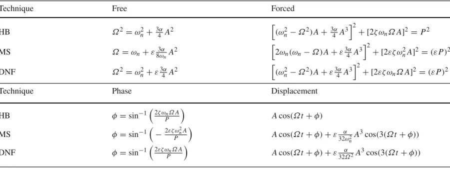
As previously mentioned, the discussion of the methods thus far has been provided so that they can be more easily compared. The system response predicted by the three methods is summarised in Table1.

By removing the bookkeeping parameter, it can be seen that the expressions for the free and forced responses in the HB and DNF method, in terms of the amplitude of the response at fundamental frequency,

A, are identical to one another.

It has been highlighted, in [4], that the free response of the MS is a linearization of that found in the HB and DNF methods, as can be found via the use of a Taylor expansion. Here, it can be seen that this remains true in the forced case. Thus, the MS solution can be considered as an approximation to the DNF and HB expressions, a point which was demonstrated to lead to divergent backbone curves in [3].

However, considering the displacement expressions in Table1, it can be seen that, by applying the same number of iterations of each method, the DNF and MS methods provide insight into the harmonic behaviour. This will not be provided by the HB method unless the trial solution is expanded to include a higher-order term.

Table 1 Summary of approximate solutions and expressions for backbone curves for the undamped, unforced Duffing oscillator

Technique Free Forced

HB Ω2_=ω2

n+3α4 A2

(ω2

n−Ω2)A+3α4 A3

2

+ [2ζ ωnΩA]2=P2

MS Ω=ωn+ε_8ω3α_nA2

2ωn(ωn−Ω)A+ε3α₄ A3 2

+ [2εζ ω2

nA]2=(εP)2

DNF Ω2_=ω2

n+ε3α4 A2

(ω2

n−Ω2)A+ε3α4 A3

2

+ [2εζ ωnΩA]2=(εP)2

Technique Phase Displacement

HB φ=sin−1 2ζ ωnΩA

P

Acos(Ωt+φ)

MS φ=sin−1 −2εζ ω2nA

P

Acos(Ωt+φ)+ε_32ωα2

nA

3_{cos(3(Ωt+φ))}

DNF φ=sin−1 2εζ ωnΩA

P

Acos(Ωt+φ)+ε α

In this study, the DNF frequency detuning, as given in Eq. (21), is applied in the MS method, resulting in the two methods giving identical expressions for the free response. In the present work, as well as considering a more general implementation of the MS method, the forced responses are considered, as outlined above.

4.1 General detuning comparison

As has already been shown, the use of a detuning is common practice in the MS method. Now, in this sec-tion, we introduce the specific detuning used in the DNF method, presented in Eq. (21), to the MS method. Recall that this is given by

ω_r2_,i =ω2_n,i+εδ=ω_n2_,i+ε(ω2_n,i−ω2_r,i). (53)

Applying this detuning in the general ε-expansion given in Eq. (8) leads to the updated expressions

ε0:(D₀2+ϒ)q₀=0,

ε1:(D₀2+ϒ)q₁+2D0D1q0+(−ϒ)q0

+Ŵq(q0,D0q0,r)=Pqr, ..

. (54)

Once more, the secular terms must be set to zero and the trial solution in Eq. (9) is again implemented, giving

jωr,i (D1Ai +AiD1φi)e+j(ωn,iT0+φi)

+(D1Ai −AiD1φi)e−j(ωn,iT0+φi)

+(ω2_n,i−ω2_r,i) Ai e+j(ωn,iT0+φi)+e−j(ωn,iT0+φi)

+Res{Γq,i Ai

2 e

+j(ωn,iT0+φi)_{+ e}−j(ωn,iT0+φi)_,

jωr,i Ai

2 e

+j(ωn,iT0+φi)_−e−j(ωn,iT0+φi)_,

e+jΩT0_+e−jΩT0_{} = P}

q,i e+j(ΩT0)+e−j(ΩT0)

.

(55)

Comparing this with the expression for the standard MS method (given in “Appendix A”), it can seen that, by removing the assumption that the response frequency is equal to the linear natural frequency, new terms arise in theε1-order equation. The inclusion of the term(ω_n2_,i−

ω_r2_,i)

Aie+j(ωn,iT0+φi)+e−j(ωn,iT0+φi)can be thought

of as a detuning term that accounts for the influence that those terms which are close to resonance have on the vibration of the system.

Collecting coefficients of e±jωr,iT0_{, Eq. (55) can be} written as

Ai(ω2n,i−ω2r,i)

e+jφi

+(D1Ai+jωr,iAiD1φi)e+jφi

+Res

Γq,i

Ai

2

e+j(ωn,iT0+φi) ,jωr,i

Ai

2 e

+j(ωn,iT0+φi)_,

e+jΩT0_−P

q,i

e+jωr,iT0_{+c.c.=0. (56)}

Similarly to the DNF method, the terms in Eq. (56) inside the square brackets are complex conjugates, so both must be equal to zero to remove the secular terms. As such, the frequency–amplitude equation can be writ-ten as

(ω_n2_,i−ω_r2_,i)

Aie+jφi+(D1Ai+jωr,iAiD1φi)e+jφi

+ResŴq Ai

2 e

+j(ωr,it+φi)_,

jωr,i Ai

2 e

+j(ωr,it+φi)_,e+jΩt

= Pq,i. (57)

Recall that the equivalent expression in the DNF method, Eq. (23), is written as

(ω_n2_,i−ω_r2_,i)Aie−jφi +Γ_u+_,i =Pu,i.

Despite the clear differences between the forms of these two expressions, it can actually be shown that they both represent the same solution. Recalling from Eq. (15) thatPq,i =Pv,i+(ω2n,i−Ω2)[e]iand noting that, for the resonant equation,[e]i = [0 0], it can be seen that Pu,i = Pq,i.

Further consideration is also given toΓ_u+_,i, which denotes the resonant terms ofŴu, including both the damping and nonlinear terms. In the detuned multiple scales (dMS) case, the resonant terms ofŴq are col-lected by the term

ResŴq Ai

2

e+j(ωr,it+φi)

,

jωr,i Ai

2

e+j(ωr,it+φi)

,e+jωr,it_.

and the combination of these terms is directly equiva-lent toΓ_u+_,i

The solution forq₁can be determined in a similar way to the standard MS method, as in Eq. (10), by solving

(−ϒ)q₁= −NRes{Ŵq}. (58)

Recall that the correspondingε1-order equation for the DNF method is

¨

h1+ϒh1+Ŵv=nu1. (59)

It can be further noted thath¨1= −h1and thatŴv− nu1 =βh1 = −NRes{Ŵq}, so that the expression in Eq. (59) can be rewritten as

(−ϒ)h1= −NRes{Ŵq}. (60)

It is immediately clear that the solutions of Eqs. (58) and (60) must be identical.

4.2 Duffing oscillator detuning comparison

These new steps can now be explored for the Duffing oscillator, beginning with the updatedε-balance, which is expressed as

ε0:D2₀q0+ω2nq0=0,

ε1:D2₀q1+ω2nq1

= −δq0−2D0D1q0−2ζ ωn(D0q1+D1q0)

−αq₀3+Pcos(ΩT0). (61)

Note that theδnotation (the SDOF equivalent toin Eq. (21)) will be used until the calculation of the final solution, so that the influence of the detuning is more readily tracked. As above, the steady-state dynamics are of interest, so the conditions in Eq. (38) are applied. Separating the real and imaginary parts now leads to the following steady-state equations

3α 4 A

3_{+Aδ =Pcos(φ),}

2ζ ωnΩA=Psin(φ). (62)

Therefore, by squaring and then summing these expres-sions, then introducing the definition ofδfrom Eq. (53), the free and forced responses are now given by

(ω_n2−Ω2)A+ε3α 4 A

32_{+ [}

2εζ ωnΩA]2=(εP)2,

(ω2_n−Ω2)+ε3α 4 A

2₌

0, (63)

respectively. Comparing these expressions with those in Eq. (49), it can be seen that the dMS and DNF forced responses are now identical, as is the case with the free response.

The harmonic part of the displacement can now be calculated using Eq. (58), giving an expression identi-cal to that of the DNF method, given in Eq. (52):

q =q0+εq1=acos(Ωt+α)

+ε α 32Ω2a

3

cos(3(Ωt+α)),

with Ω =

ω2_n+ε3α 4 a

2_{. (64)}

5 Results

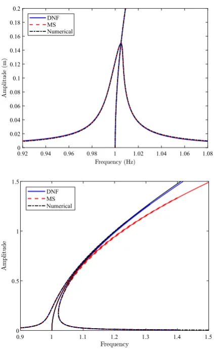
Figure1shows graphical representations of the responses in Table 1; the bookkeeping parameter is simply removed from the expressions, so the HB curve is identical to that given by the DNF/dMS methods. The ‘Numerical’ backbone curve in Fig.1has been found using numerical continuation [2]. In this figure, the following parameter values have been used:ωn = 1, α = 0.6, with ζ = 0.005, P = 0.0015 in the first case andζ =0.0015,P =0.005 in the second. These two forcing cases allow the influence of this detuning to be considered at both high and low amplitudes. In the first case, it can be seen that the variation between the techniques is very small. In fact, when the system is forced at low levels, it could be argued that the choice of method has a negligible influence on the response prediction.

0.92 0.94 0.96 0.98 1 1.02 1.04 1.06 1.08 0

0.02 0.04 0.06 0.08 0.1 0.12 0.14 0.16 0.18 0.2

DNF MS Numerical

0.9 1 1.1 1.2 1.3 1.4 1.5

0 0.5 1 1.5

DNF MS Numerical

Fig. 1 Free and forced responses atε1-order, for the HB, DNF, and MS methods (without the newly applied detuning), and numerically continued (Full) solutions. The first panel displays the results from Case 1:ζ = 0.005, P = 0.0015, the second from Case 2:ζ=0.0015,P=0.005

which they do so. While the DNF/dMS methods remain close to the numerical solution across the considered range, the MS method begins to diverge at approxi-matelyΩ = 1.1 Hz, which represents a shift in fre-quency of roughly 10%. When this point is reached, the MS method begins to underestimate the displacement. It has been shown that, by choosing the detuning found in the DNF method, it is possible to remove the under-prediction of the forced response; in Fig.1, the updated MS curve is identical to that of the DNF method.

5.1 Considerations for users

As has shown in the previous sections, by choosing a suitable frequency detuning, it is possible to achieve

identical results when applying any of the techniques discussed to the example system. As such, it could be concluded that the user may choose the technique with which they are most familiar and ensure that the accu-racy of the solutions will not be compromised. While there may be some truth to this assertion, the discussion provided in this study alludes to further considerations that could be taken.

The HB method has been demonstrated to be a much simpler technique than the others considered; it is arguably for this reason that it has been more widely applied, particularly in those cases that have seen a more algorithmic approach taken for larger sys-tems. As a result of this simplicity, the method lacks the bookkeeping parameter used by the MS and DNF techniques. As has been previously discussed, this per-turbation strategy not only measures the relative con-tribution of each term, but actually informs the user as to the neighbourhood of to linear natural frequency in which they may have confidence in the accuracy of the results. Thus, the HB should be seen as an effective method for gaining a quick understanding of the nonlinear behaviour, but is likely to be most useful when the exact values of the solution are not important.

The results presented in this paper, along with those of [3], have demonstrated that the MS and DNF are able to provide identical results. Given that the implemen-tation of the two techniques requires a similar number of steps, this leaves the user to make a decision based on the nuances of the particular system they are con-sidering. A key benefit of the MS has always been its ability to model transient behaviour. Since this is not affected by the frequency tuning, this asset still holds true. Meanwhile, the DNF technique utilises a matrix formulation to effectively track the resonant and non-resonant terms, a strategy that may prove useful in more complex structures with multiple harmonics. In sum-mary, the results of the present work provide the user with two accurate options, which will suit a wide array of potential structures.

6 Conclusions

study of such techniques. In particular, the harmonic balance, multiple scales, and direct normal forms meth-ods have been considered. In an initial comparison, it has been shown that the HB and DNF give identi-cal solutions for the Duffing oscillator, although the inclusion of a bookkeeping parameter in the latter pro-vides the potential for a simpler management of weak terms in more complex structures. Additionally, the matrix formulation of the DNF method also reveals the harmonic components of the behaviour, whereas this requires the introduction of a more complex trial solu-tion in the HB method. In previous works, it has been shown that the free vibration expression given by the MS is a linearization of the HB/DNF solution. In this work, it has been shown that this property also holds true for the forced response.

To expand this comparison, the previously devel-oped detuned multiple scales method is extended to include forced responses. Furthermore, an alternative form of the MS method is applied, demonstrating the broader applicability of the comparison. By consider-ing the widely applied derivative expansion version of the MS method, it has been shown that, for a gen-eral nonlinear system, the analytical solutions of the forced, damped equations are, once more, identical in the DNF and dMS methods. This is an important result, as it means that, regardless of the method chosen, the user has the potential to capture complex nonlinear behaviour in forced structures (such as hysteresis and internal resonance) to the same level of accuracy.

Particular attention has been given to the influ-ence that the forcing and damping terms have on the divergence of the MS and DNF/dMS responses. In models with lower forcing and/or higher damping, it has been seen that the difference between these solutions is effectively negligible. However, as the forcing grows, the non-detuned MS method begins to under-predict the displacement, demonstrating that there is a region in which the linearization is valid and that the prediction may become inaccurate away from this.

Funding Funding was provided by Engineering and Physical Sciences Research Council (Grant No. EP/K005375/1).

Compliance with ethical standards

Conflict of interest The authors declare that they have no con-flict of interest.

Open Access This article is distributed under the terms of the Creative Commons Attribution 4.0 International License (http://creativecommons.org/licenses/by/4.0/), which permits unrestricted use, distribution, and reproduction in any medium, provided you give appropriate credit to the original author(s) and the source, provide a link to the Creative Commons license, and indicate if changes were made.

Appendix A

Once theε-expansion in Eq. (8) has been established, theε0-order can be solved to give

q0,i =

Ai(T1,T2, . . .)

2

e+j(ωr,iT0+φi(T1,T2, ...))_+e−j(ωr,iT0+φi(T1,T2, ...))_,

(A.1)

where Ai andφi denote the amplitude and phase of the fundamental response of theith mode, respectively. Thisε0-order solution can now be applied to theε1 -order terms in Eq. (8) to give

(D₀2+ω2_n,i)q1,i

= −jωn,i (D1Ai+AiD1φi)e+j(ωn,iT0+φi)

−(D1Ai−AiD1φi)e−j(ωn,iT0+φi)

−Γq,i Ai

2 e

+j(ωn,iT0+φi)_+e−j(ωn,iT0+φi)_,

jωn,i Ai

2 e

+j(ωn,iT0+φi)_−e−j(ωn,iT0+φi)_,

e+jΩt+e−jΩt+Pq,irp. (A.2)

Now, the secular terms—i.e., those that respond at ωn,i—must be set to zero. The reason for this is that the homogeneous form of Eq. (A.2) is given by (D₀2+)q1 =0. As such, the trial solution must be

equal to the trial solution forq0. Therefore, a failure

to remove the secular terms would lead to a divergent solution. Removing the secular terms in Eq. (A.2) leads to the expression

jωn,i (D1A0,i+A0,iD1φi)e+j(ωn,iT0+φi)

+(D1A0,i −A0,iD1φi)e−j(ωn,iT0+φi)

+ResΓq,i A0,i

2 e

jωn,i A0,i

2 e

+j(ωn,iT0+φi)_−e−j(ωn,iT0+φi)_,

e+jΩt +e−jΩt−Pq,irp

=0, (A.3)

where Res{•}denotes the resonant terms of •. This secular equation can now be solved to find expressions for the amplitude and phase terms. This is done by separating the real and imaginary parts of the equation, then setting the coefficients of e±j(ωn,iT0+φi) _{in each} of those to zero. The solutions for A0,i andφi can be applied in the non-resonant equation:

(D2₀+ω2_n,i)q1,i

= −NRes

Ŵq

A0,i

2 e

+j(ωn,iT0+φi)_+e−j(ωn,iT0+φi)_,

×jωn,i

A0,i

2 e

+j(ωn,iT0+φi)_−e−j(ωn,iT0+φi)_,

×e+jΩt+e−jΩt, (A.4)

where NRes{•}denotes the non-resonant terms of •. This equation can then be solved to findq₁. Now, the solutions forq₀andq₁can be applied to theε2-order expression to findq₂. The process is the same and, therefore, not shown here, but details can be found in [3].

Appendix B

Recall that Eq. (20) is given by

(εh¨1+ε2h¨2+ · · ·)+ (εϒh1+ε2ϒh2+ · · ·)

+εŴv(u+εh,u˙+εh,˙ r)

−(εŴu,1+ε2Ŵu,2+ · · ·)+Pur−Pvr=0.(B.1)

Here, we apply a Taylor expansion toŴv(u+εh,u˙+ εh,˙ r), and simplify using the notation

Ŵv,1=Ŵv,

Ŵv,2=

−ϒ+ ∂

∂uŴv

h1+

∂

∂u˙Ŵv

˙

h1.

Then, the vector u∗_i, which captures all the possible polynomial terms which could arise in the expansion ofŴu, is used to introduce the following matrix formu-lations

Ŵv,i(u,u,˙ r)= [Γv,i]u∗i(up,um,r),

Ŵu,i(u,u,˙ r)= [Γu,i]u∗i(up,um,r),

hi(u,u,˙ r)= [hi]u∗i(up,um,r), (B.2)

where[Γv,i],[Γu,i], and[hi]areN ×Ni matrices of invariant coefficients for the corresponding time-dependent terms inu_i∗. Thus, fori ≥1, theεi homo-logical equation is given by

[hi] ¨u∗i +Υ[hi]u∗i + [Γv,i]u∗i = [Γu,i]u∗i. (B.3)

By consideration of theui vector, it is possible to find a solution foru. First, theℓth element ofu∗_i is written as

u∗_i,ℓ=rmppi,ℓr mmi,ℓ m

N

n=1 uspnpi,ℓ,nu

smi,ℓ,n mn =Ui∗,ℓe

j(ω∗_i,ℓt−φ_i∗_,ℓ)

,

(B.4)

where

U_i∗_,ℓ= N

n=1

_U

n 2

(sp,i,ℓ,n+sm,i,ℓ,n) ,

φ_i∗_,ℓ= N

n=1

(sm,i,ℓ,n−sp,i,ℓ,n)φn,

and

ω∗_i,ℓ =(mp,i,ℓ−mm,i,ℓ)Ω+

N

n=1

(sp,i,ℓ,n−sm,i,ℓ,n)

ωr,n.

These new variables can be applied in Eq. (B.3) so that element {k, ℓ} of[Γv,i]can be written as

[Γv,i]k,ℓ= [Γu,i]k,ℓ+βi,k,ℓ[hi]k,ℓ, (B.5)

where

βi,k,ℓ= [ω∗i,ℓ]

2_−ω2

r,i, (B.6)

defines theN×Ni matrixβi. Therefore, if[ω∗i,ℓ]2= ω_r2_,i, thenβi,k,ℓ = 0. As such,βi can be considered as a matrix that determines the resonance of the terms defined by[Γv,i].

Now,

[Γv,i]k,ℓ= [Γu,i]k,ℓ, [hi]k,ℓ=0, if βi,k,ℓ=0, (B.7)

[Γv,i]k,ℓ=0, [hi]k,ℓ=

[Γu,i]k,ℓ βi,k,ℓ

Applying these conditions, theith resonant equation can be expressed as

(ω2_n,i−ω2_r,i)Uie−jφi +Γui+−P

+

ui

e+jωr,it

+(ω2_n,i−ω2_r,i)Uie+jφi +Γui−−P

−

ui

e−jωr,it _=0,

(B.9)

whereP_ui+andP_ui−denote elements{i,1}and{i,2}of Pu, respectively. The variablesΓ_ui+andΓ_ui−arise in the decomposition

Γui =Γui+e

+jωr,it_+Γ− uie

−jωr,it_{. (B.10)}

The terms in Eq. (B.9) which are contained in square brackets are complex conjugates of one another and, for this equality to hold, it is necessary for both of these to be equal to zero. Therefore, the frequency–amplitude relationship is given by

(ω2_n,i−ω2_r,i)Uie−jφi +Γui+= P

+

ui, (B.11)

which can be solved to find the fundamental response of the system.

References

1. Wagg, D.J., Neild, S.A.: Nonlinear Vibration with Control. Springer, Berlin (2009)

2. Doedel, E.J., Champneys, A.R., Fairgrieve, T.F., Kuznetsov, Y.A., Dercole, F., Oldeman, B.E., Paffenroth, R.C., Sand-stede, B., Wang, X.J., Zhang, C.: Auto-07p: Continuation and bifurcation software for ordinary differential equations, Montreal, Concordia University, Canada, (2008). http:// cmvl.cs.concordia.ca. Accessed 16 Dec 2018

3. Elliott, A.J., Cammarano, A., Neild, S.A., Hill, T.L., Wagg, D.J.: Comparing the direct normal form and multiple scales methods through frequency detuning. J. Sound Vib. 94, 2919–2935 (2018)

4. Elliott, A.J., Cammarano, A., Neild, S.A.: Comparing ana-lytical approximation methods with numerical results for nonlinear systems. In: G. Kerschen (Ed.), Conference Pro-ceedings of the Society for Experimental Mechanics Series, Springer, (2017)

5. Hill, T.L., Neild, S.A., Barton, D.: Comparing the direct normal form method with harmonic balance and the method of multiple scales. Proc. Eng.199, 869–874 (2017) 6. Neild, S.A., Wagg, D.J.: A generalized frequency detuning

method for multi-degree-of-freedom oscillators with non-linear stiffness. Nonnon-linear Dyn.73, 649–663 (2013)

7. Sharma, S., Coetzee, E.B., Lowenberg, M.H., Neild, S.A., Krauskopf, B.: Numerical continuation and bifurcation anal-ysis in aircraft design: an industrial perspective. Philols. Trans. R. Soc. A373, 20140406 (2015)

8. Cammarano, A., Neild, S.A., Burrow, S.G., Inman, D.J.: The bandwidth of optimized nonlinear vibration-based energy harvesters. Smart Mater. Struct.23, 055019 (2014) 9. Peeters, M., Viguié, R., Sérandour, G., Kerschen, G.,

Golin-val, J.-C.: Nonlinear normal modes, part ii: toward a prac-tical computation using numerical continuation techniques. Mech. Syst. Signal Process.23, 195–216 (2009)

10. Hill, T.L., Cammarano, A., Neild, S.A., Wagg, D.J.: Inter-preting the forced responses of a two-degree-of-freedom nonlinear oscillator using backbone curves. J. Sound Vib. 349, 276–288 (2015)

11. Hill, T.L., Neild, S.A.: Cammarano, An analytical approach for detecting isolated periodic solution branches in weakly nonlinear structures. J. Sound Vib.379, 150–165 (2016) 12. Haller, G., Ponsioen, S.: Nonlinear normal modes and

spec-tral submanifolds: existence, uniqueness and use in model reduction. Nonlinear Dyn.86, 1493–1534 (2016) 13. Özer, M.B., Özgüven, H.N.: A new method for localization

and identification of non-linearities in structures, In: Pro-ceedings of ESDA 2002: 6thBiennial Conference on Engi-neering Systems, (2002)

14. Aykan, M., Özgüven, H.N.: Parametric identification of nonlinearity in structural systems using describing function inversion. Mech. Syst. Signal Process.40, 356–376 (2013) 15. Narayanan, M.D., Narayanan, S., Padmanabhan, C.: Para-metric identification of nonlinear systems using multiple tri-als. Nonlinear Dyn.48, 341–360 (2007)

16. Kerschen, G., Peeters, M., Golinval, J.C., Vakakis, A.F.: Nonlinear normal modes, part i: a useful framework for the structural dynamicist. Mech. Syst. Signal Process.23, 170– 194 (2009)

17. Detroux, T., Renson, L., Masset, L., Kerschen, G.: The har-monic balance method for bifurcation analysis of large-scale nonlinear mechanical systems. Comput. Methods Appl. Mech. Eng.296, 18–38 (2015)

18. Rahman, Z., Burton, T.D.: On higher order methods of mul-tiple scales in non-linear oscillations-periodic steady state response. J. Sound Vib.133, 369–379 (1989)

19. Wang, W., Xu, J.: Multiple scales analysis for double hopf bifurcation with 1:3 resonance. Nonlinear Dyn.66, 39–51 (2011)

20. Luongo, A., Egidio, A.D.: Perturbation methods for bifur-cation analysis from multiple nonresonant complex eigen-values. Nonlinear Dyn.14, 193–210 (1997)

21. Luongo, A., Paolone, A., Egidio, A.D.: Multiple timescales analysis for 1:2 and 1:3 resonant hopf bifurcations. Nonlin-ear Dyn.34, 269–291 (2003)

22. Luongo, A., Paolone, A.: Bifurcation equations through multiple-scales analysis for a continuous model of a planar beam. Nonlinear Dyn.41, 171–190 (2005)

23. Benedettini, F., Rega, G., Alaggio, R.: Non-linear oscilla-tions of a four-degree-of-freedom model of a suspended cable under multiple internal resonance conditions. J. Sound Vib.182, 775–798 (1995)

25. Nayfeh, A.H.: Quenching of primary resonance by a super-harmonic resonance. J. Sound Vib.92, 363–377 (1982) 26. Cammarano, A., Hill, T.L., Neild, S.A., Wagg, D.J.:

Bifur-cations of backbone curves for systems of coupled nonlin-ear two mass oscillator. Nonlinnonlin-ear Dyn.77(1–2), 311–320 (2014)

27. Neild, S.A., Champneys, A., Wagg, D.J., Hill, T.L., Cam-marano, A.: The use of normal forms for analysing nonlinear mechanical vibrations. Philols. Trans. R. Soc. A373(2051), 20140404 (2015)

28. Lamarque, C.-H., Touzé, C., Thomas, : An upper bound for validity limits of asymptotic analytical approaches based on normal form theory. Nonlinear Dyn.70, 1931–1949 (2012) 29. Eugeni, M., Dowell, E.H., Mastroddi, F.: Post-buckling longterm dynamics of a forced nonlinear beam: a pertur-bation approach. J. Sound Vib.333, 2617–2631 (2014) 30. Hill, T.L., Cammarano, A., Neild, S.A., Barton, D.:

Identi-fying the significance of nonlinear normal modes. Proc. R. Soc. Lond. A: Math. Phys. Eng. Sci.473, 20160789 (2017) 31. Shaw, A., Hill, T., Neild, S., Friswell, M.: Periodic responses of a structure with 3:1 internal resonance. Mech. Syst. Signal Process.81, 19–34 (2016)

32. Hill, T.L., Green, P.L., Cammarano, A., Neild, S.A.: Fast bayesian identification of a class of elastic weakly nonlinear systems using backbone curves. J. Sound Vib.360, 156–170 (2016)

33. Neild, S.A., Wagg, D.J.: Applying the method of normal forms to second-order nonlinear vibration problems. Proc. R. Soc. Lond. A467(2128), 1141–1163 (2011)

34. Xin, Z., Neild, S.A., Wagg, D.J.: The selection of the lin-earized natural frequency for the second-order normal form method. In: ASME 2011 International Design Engineering Technical Conferences and Computers and Information in Engineering Conference, pp. 1211–1218, (2011)

35. Nayfeh, A.H.: Introduction to Perturbation Techniques. Wiley, Hoboken (1981)

36. Nayfeh, A.H., Mook, D.T.: Nonlinear Oscillations. Wiley, Hoboken (1979)

37. Strogatz, S.H.: Nonlinear Dynamics and Chaos. Perseus Books, New York (1994)

38. Beléndez, A., Hernández, A., Beléndez, T., Álvarez, M.L., Gallego, S., Ortuño, M., Neipp, C.: Application of the har-monic balance method to a nonlinear oscillator typified by a mass attached to a stretched wire. J. Sound Vib.302, 1018– 1029 (2007)

39. Ghadimi, M., Kaliji, H.D.: Application of the harmonic bal-ance method on nonlinear equations. World Appl. Sci. J.22, 532–537 (2013)

40. Nayfeh, A.: Perturbation Methods. Wiley, Hoboken (2000) 41. Kovacic, I., Brenna, J.J.: The Duffing Equation: Nonlinear

Oscillators and their Behaviour. Wiley, Hoboken (2011)