A Cartesian-grid Collocation Technique with Integrated Radial Basis Functions for mixed boundary value problems
Phong Le1, Nam Mai-Duy1, Thanh Tran-Cong1,3 and Graham Baker2
1CESRC, University of Southern Queensland, Toowoomba, QLD 4350, Australia. 2DVC(S), University of Southern Queensland, Toowoomba, QLD 4350, Australia.
Abstract: In this paper, high order systems are reformulated as first order systems which are then numerically solved by a collocation method. The collocation method is based on Carte-sian discretisation with 1D-integrated radial basis function networks (1D-IRBFN) [1]. The present method is enhanced by a new boundary interpolation technique based on 1D-IRBFN which is in-troduced to obtain variable approximation at irregular points in irregular domains. The proposed method is well suited to problems with mixed boundary conditions on both regular and irregular domains. The main results obtained are (a) the boundary conditions for the reformulated problem are of Dirichlet type only; (b) the integrated RBFN approximation avoids the well known reduc-tion of convergence rate associated with differential formulareduc-tions; (c) the primary variable (e.g. displacement, temperature) and the dual variable (e.g. stress, temperature gradient) have similar convergence order; (d) the volumetric locking effects associated with incompressible materials in solid mechanics are alleviated. Numerical experiments show that the proposed method achieves very good accuracy and high convergence rates.
Keywords: RBF, collocation method, elasticity, Cartesian grid, mixed formulation, first order system, volumetric locking, incompressibility.
1
INTRODUCTION
Traditional finite element methods (FEM) [2] and boundary element methods (BEM) have been based on weak-form formulations. Recently, weak-form meshless (meshfree) methods are being developed as an alternative approach. Weak-form methods have the following advantages [3, 4] a) they have good stability and reasonable accuracy for many problems; b) Neumann bound-ary conditions can be naturally and conveniently incorporated into the same weak-form equation. However, elements have to be used for the integration of a weak form over the global problem domain [5] and the numerical integration is still computationally expensive for these weak-form methods. On the other hand, collocation methods are based on strong-form governing equations and have been found to possess the following attractive advantages [3, 6–9] a) they are compu-tationally efficient since there is no need for numerical integration of the governing equations; b) the implementation is simple; c) implementation of Dirichlet boundary conditions is very straight-forward. However, the strong-form approach is less stable due to the pointwise nature of error minimisation and results in typically poorer accuracy for problems governed by partial differential
3
equations with Neumann-type boundary conditions such as solid mechanics problems with traction (natural) boundary conditions. Furthermore, some strong-form methods such as finite difference and pseudo spectral methods are restricted to rectangular domains.
Therefore, many efforts have been made to develop techniques for handling the Neumann-type boundary conditions such as direct collocation, fictitious points, regular grids, and dense nodes in the derivative boundaries [10]; Hermite-type collocation [11, 12]. Recently, Zhang et al [13] suggested Least-squares collocation meshless method which can improve the accuracy of the solution in comparison with the one of standard collocation method. Onate et al [14] introduced a stabilization technique by adding artificial terms in both governing equations and Neumann boundary conditions, however, these terms only serve the stabilization purpose and their suitability is restricted to some special problems. Liu and Gu [15, 16] proposed a meshfree weak-strong-form method, in which the weak form is applied to the subdomain concerned with Neumann boundary conditions and strong form to the one with Dirichlet boundary conditions. Pan et al [17] presented meshless Galerkin least-squares method by making use of Galerkin method in the boundary domain and least-squares method in the interior domain. Hu et al [18, 19] introduced the weighted radial basis collocation method in which the residual error on the Neumann boundary is treated by a proper scaling weight. Atluri et al [20, 21] proposed a “mixed” collocation technique, however, stable solutions are obtained with resort to the local weak form at nodal points for stress and the penalty method for Neumann boundary conditions. Libre et al [22] proposed a stabilized collocation scheme for radial basis functions (RBF) by increasing the shape parameter of RBF and the number of collocation points around the Neumann boundaries, however, increasing the shape parameter leads to increased ill-conditioning. Lee and Yoon [23] introduced generalized diffuse derivative in a collocation method.
In recent years, increasing attention has been drawn to the development of first-order system formulation. In earlier works of Cai et al [24, 25], they developed the theory of first-order system formulation for general second-order elliptic PDEs. This methodology has been then extended to the Stokes equations [26] in two and three dimensions, elasticity problems [27–29], and boundary value problems with Robin boundary conditions [30]. However, the efforts have been mainly concentrated in using weak-form Galerkin or weak-form least-squares formulation. For example, Jiang and Wu [31] presented the least-squares finite element method; Park and Youn [32] introduced the least-squares meshless method and Kwon et al [33] subsequently extended this method to elasticity problems. Relatively few works have been done with first-order system formulation based on strong-form method.
differential formulations; (c) the primary variable (e.g. displacement, temperature) and the dual variable (e.g. stress, temperature gradient) have similar convergence order; (d) the volumetric locking effects associated with incompressible materials in solid mechanics are alleviated without any extra effort. (In contrast, in meshless weak form approaches, special treatments need to be done in the case of incompressible materials, for instance, Dolbow and Belytschko [37] introduced reduced integration procedure, Chen et al [38] proposed the pressure projection technique for the purpose of alleviating the incompressible locking.) Moreover, the generation of a Cartesian grid is a straightforward task and therefore the cost associated with spatial discretisation is greatly re-duced in comparison with that associated with FE generation. Numerical experiments show that the proposed method achieves very good accuracy and high convergence rates.
The remainder of the paper is organized as follows. The physical problem and its mathematical model are defined in section 2. The numerical formulation for the mathematical model is presented in section 3. The proposed method is illustrated by numerical examples in section 4. Section 5 concludes the paper.
2
PROBLEM FORMULATIONS
2.1
First-order systems
Cai and co-workers [24–29] studied the behaviour of equivalent first-order formulations of second-order systems and found that FE implementation of such first-second-order systems yields uniform optimal performance. The higher-order differential equations are transformed to first-order differential equations by introducing new dual variables. Both primary and dual variables are independently interpolated and have shape functions of the same order. It is noticed that in general all higher-order differential equations can be transformed to first-higher-order differential equations [24, 30]. The resulting first-order system of governing equations can be written as follows.
Lu=f, in Ω (1)
Bu=g, on Γ (2)
where Ω is a bounded domain in Rd, d = 1,2,3, Γ the boundary of Ω, L is a first-order linear
differential operator
Lu=L0u+
d
X
i=1
Li
∂u ∂xi
, (3)
in which uT = [u1, u2, ..., um] is a vector of m unknown functions (including primary and dual
variables) of xT = [x1, x2, ..., xd], Li the coefficient matrices which characterize the differential
2.2
Two-dimensional Poisson equation
Consider the following two-dimensional Poisson equation
∂2φ(x, y) ∂x2 +
∂2φ(x, y)
∂y2 =f(x, y) in Ω, (4a)
φ(x, y) =g(x, y) on ΓD, (4b)
∂φ(x, y)
∂n =h(x, y) on ΓN, (4c)
where Ω is a bounded domain inR2, ΓD and ΓN the boundary of Ω on which the Dirichlet and
Neumann boundary condition are imposed, respectively, n= (nx, ny)T the outward unit normal
on ΓN, andf,g andhthe given functions on Ω, ΓD and ΓN, respectively.
A first-order formulation is obtained by introducing the dual variables in (4) as follows
∂φ(x, y)
∂x −ξ(x, y) = 0 in Ω and on ΓD [
ΓN, (5a)
∂φ(x, y)
∂y −η(x, y) = 0 in Ω and on ΓD [
ΓN, (5b)
∂ξ(x, y) ∂x +
∂η(x, y)
∂y =f(x, y) in Ω and on ΓD [
ΓN, (5c)
φ(x, y) =g(x, y) on ΓD, (5d)
nxξ+nyη=h(x, y) on ΓN. (5e)
2.3
Linear elasticity problems
Consider the following two-dimensional problem on the domain Ω bounded by Γ = ΓuSΓt
∇ ·σ=b in Ω, (6a)
u=¯u on Γu, (6b)
σ·n=¯t on Γt, (6c)
in whichσ is the stress tensor, which corresponds to the displacement fielduand bis the body
force, n the outward unit normal on Γt. The superposed bar denotes prescribed value on the
boundary.
The governing equations (6) are closed when a constitutive relation is specified for σ. Here
the linear Hooke’s law is used to describe the σ−u relation. By choosing displacement u as
are written for plane stress case as follows
∂u ∂x−
1 Eσx+
µ
Eσy= 0, (7a)
∂v ∂y +
µ Eσx−
1
Eσy= 0, (7b)
∂u ∂y +
∂v ∂x−
2(1 +µ)
E τxy= 0, (7c)
∂σx
∂x + ∂τxy
∂y =bx, (7d)
∂τxy
∂x + ∂σy
∂y =by, (7e)
u=¯u on Γu, (7f)
σ·n=¯t on Γt, (7g)
whereµis Poisson ratio andE Young’s modulus. By introducing the dimensionalless stress tensor s=σ/E, the above first-order system can be rewritten as follows
∂u
∂x−sx+µsy= 0, (8a)
∂v
∂y+µsx−sy= 0, (8b)
∂u ∂y+
∂v
∂x −2(1 +µ)sxy= 0, (8c)
∂sx
∂x + ∂sxy
∂y =bx, (8d)
∂sxy
∂x + ∂sy
∂y =by, (8e)
u=u¯ on Γu, (8f)
s·n=¯t on Γt. (8g)
3
NUMERICAL FORMULATIONS
In a number of methods, approximations of spatial derivatives are less accurate because differ-entiation magnifies errors. Madych [39] estimated that MQ-RBF enjoys spectral convergence of order O(λah), where 0 < λ < 1, a is the shape parameter and h is the maximum mesh size.
A differential formulation with spatial derivatives of orderδ reduces convergence rate of MQ to O(λah−δ). To increase the accuracy and the convergence rate of MQ, several approaches have been
proposed such as a) increasingaor decreasing hor both [22], b) integrated methods of Mai-Duy and Tran-Cong [1, 40–42] and c) using higher order MQ, e.g. ϕi= (ri2+a2i)β, whereβ > 12 [43].
3.1
1D-IRBFN approximation
For the sake of completeness, the 1D-IRBFN approximation for 2D problems in [1] is reproduced as follows. Consider a grid point/regular pointx (x= (x, y)T) (Figure 1). Along the horizontal
line passing through this point, one can use IRBFNs to construct the expressions for the function uand its derivatives with respect tox. The construction process can be described as follows. The second-order derivative of uis first decomposed into RBFs; the RBF network is then integrated twice to obtain the expressions for the first-order derivative and the function itself
∂2u(x) ∂x2 =
N
X
i=1
w(i)g(i)(x) =
N
X
i=1
w(i)H(i)
[2](x), (9)
∂u(x) ∂x =
N
X
i=1
w(i)H[1](i)(x) +c1, (10)
u(x) =
N
X
i=1
w(i)H(i)
[0](x) +c1x+c2, (11)
whereN is the number of nodal points (interior and boundary points) on the line,{w(i)}N i=1 are RBF weights to be determined, {g(i)(x)}N
i=1 are known RBFs, H[1](x) = R
H[2](x)dx, H[0](x) = R
H[1](x)dx, and c1 and c2 are integration constants. Here, it is referred to as a second-order 1D-IRBFN scheme, denoted by IRBFN-2. The present study employs multiquadrics (MQ) whose form is
g(i)(x) =q(x−c(i))2+a(i)2, (12)
wherec(i)anda(i)are the centre and the RBF width/shape parameter of theith RBF. The width of theith RBF can be determined according to the following simple relation
ai=βdi, (13)
whereβ is a factor,β >0, anddi is the distance from theithcentre to its nearest centre. The set
of centres is chosen to be the same as the set of the collocation points. It is more convenient to work in the physical space than in the network-weight space. The values of the variableuat the N nodal points can be expressed as
u(x(1)) =
N
X
i=1
w(i)H[0](i)(x(1)) +c1x(1)+c2, (14)
u(x(2)) =
N
X
i=1
w(i)H(i) [0](x
(2)) +c1x(2)+c2, (15)
· · · ·
u(x(N)) =
N
X
i=1
w(i)H[0](i)(x(N)) +c1x(N)+c2, (16)
or in a matrix form
b u=H
x
1 2 3 N
where ub= (u(1), u(2),· · · , u(N))T,
b
w = (w(1), w(2),· · ·, w(N))T,
b
c = (c1, c2)T, and H is a known
matrix of dimensionN×(N+ 2) defined as
H=
H[0](1)(x(1)) H(2)
[0](x(1)) · · · H (N)
[0] (x(1)) x(1) 1 H[0](1)(x(2)) H(2)
[0](x(2)) · · · H (N)
[0] (x(2)) x(2) 1
· · · ·
H[0](1)(x(N)) H(2) [0](x
(N)) · · · H(N) [0] (x
(N)) x(N) 1 .
Using the singular value decomposition (SVD) technique, one can write the RBF coefficients in-cluding two integration constants in terms of the meaningful nodal variable values
b w bc
=H−1bu. (18)
It is noted that the purpose of using SVD here is to provide a solution whose norm is the smallest in the least-squares sense. By substituting (18) into (9)-(11), the values ofuand its derivatives with respective toxat pointxcan now be computed by
∂2u(x) ∂x2 =
H[2](1)(x), H[2](2)(x),· · · , H[2](N)(x),0,0H−1u,b (19)
∂u(x) ∂x =
H[1](1)(x), H[1](2)(x),· · · , H[1](N)(x),1,0H−1u,b (20)
u(x) =H[0](1)(x), H[0](2)(x),· · · , H[0](N)(x), x,1H−1bu. (21)
Substituting a discrete approximation ofuand its first-order derivatives as given in (21) and (20) into (1) and (2) and using the collocation method at all the nodes of Ω and Γ, one obtains the linear algebraic system as presented below.
LetNΩdenote the number of interior nodes,NDthe number of nodes on the Dirichlet boundary,
NN the number of nodes on the Neumann boundary,mp the number of primary unknowns and
md the number of dual unknowns associated with a node, the number of nodal unknowns is
generally (NΩ+ND+NN)(mp+md). If one collocates the governing equations (1) atNΩinterior
nodes and the boundary conditions (2) at (ND+NN) boundary nodes, the number of obtained
equations is (NΩ(mp+md) +NDkD+NNkN), where kD and kN are the number of equations
from the boundary conditions per node on the Dirichlet and Neumann boundaries, respectively. Consequently, the number of equations is less than the number of unknowns on the boundaries since kD andkN are usually less thanmp+md, respectively. To overcome this deficiency, we propose
a new scheme for the treatment of boundary conditions of the first-order collocated system as follows. The governing equations (1) is collocated at all the interior and boundary nodes, yielding (NΩ+ND+NN)(mp+md) equations. The boundary conditions are imposed by collocating equation
(2) at all the boundary nodes, i.e. the obtained system has (NΩ+ND+NN)(mp+md) +NDkD+
NNkN equations. The final system is obtained by removingNDkD+NNkN appropriate equations
corresponding to the governing equations collocated at the boundary nodes. Consequently, the number of equations of the resulting system is equal to the number of nodal unknowns and it can be rewritten in a compact form
Another possible treatment of the boundary conditions in this case is that both governing equations (1) and boundary conditions (2) are imposed at all the boundary nodes. As a result, the number of equations is greater than the number of unknowns, and the resulting system can be solved in the least-square sense. However, our numerical study indicates that the least-squares scheme provides poorer accuracy than the proposed scheme.
3.2
Irregular boundary interpolation technique
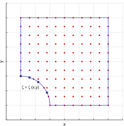
Consider a representative irregular boundary as shown in Figure 2, Cartesian grid based methods generally are not able to represent irregular nodes (e.g. points 1, N in Figure 2) on this boundary and the 1D-IRBFN is no exception. To interpolate variables at irregular points, a new boundary interpolation technique based on 1D-IRBFN is introduced as follows.
If the curve (irregular boundary) is a function ofxand y, i.e. ζ =ζ(x, y), and x=x(ζ) and y =y(ζ), a function value f =f(x, y) is invariant with respect to ζ coordinate system (i.e. the natural coordinate system)
f =f(x, y) =f[x(ζ), y(ζ)] =f(ζ). (23) From (23), we have the following relation
∂f ∂ζ = ∂f ∂x ∂x ∂ζ + ∂f ∂y ∂y
∂ζ, (24)
which can be used for determining ∂f∂x (or ∂f∂y) at the irregular nodes if ∂x ∂ζ, ∂y ∂ζ and ∂f ∂y (or ∂f ∂x) are
known. In general, f(ζ), x(ζ), y(ζ) and their corresponding derivatives can be approximated by 1D-IRBFN. To illustrate the proposed scheme, let the irregular boundary be a circle, we need to determine ∂f∂x at the “square” nodes on the circle (Figure 2). We have the relations
ζ(x, y)≡θ(x, y) = arctan(y/x), (25)
x=rcos(θ), y=rsin(θ), (26)
f(θ) =f[x(θ), y(θ)] =f, (27)
∂f ∂θ = ∂f ∂x ∂x ∂θ + ∂f ∂y ∂y
∂θ, (28)
where r is the radius of the circle. In general, if f(θ) is not available analytically, it can be approximated by a 1D-IRBFN, ∂f∂y (∂f∂x) of these nodes can be approximated along the vertical (horizontal) lines. Therefore, ∂f∂x (∂f∂y) can be easily obtained by using (28).
4
NUMERICAL EXAMPLES
For error estimation and convergence studies, the discrete relative L2 norm of errors of primary and dual variables are defined as
Lφ2 = r
PM i=1
φ(ei)−φ(i)
2
r PM
i=1
φ(ei)
x
y
[image:10.595.274.474.139.342.2]ζ = ζ (x,y)
Figure 2: 1D interpolation scheme for irregular boundary
Lξη2 = s
PM i=1
ξe(i)−ξ(i)
2
+ηe(i)−η(i)
2
s PM
i=1
ξ(ei)
2 +η(ei)
2 , (30)
for Poisson equation and
Lu2= r
PN i=1
(ux)
(i)
e −(ux)(i)
2 (uy)
(i)
e −(uy)(i)
2
s PN
i=1
(ux)(ei)
2
+(uy)(ei)
2 , (31)
Lσ 2 = s PM i=1
(sx)(ei)−s(xi)
2
+(sy)(ei)−s(yi)
2
+(sxy)(ei)−s(xyi)
2
s PM
i=1
(sx)
(i)
e
2
+(sy)
(i)
e
2
+(sxy)
(i)
e
2 , (32)
for elasticity problems, where M is the number of unknown nodal values and the subscript “e” denotes the exact solution. The convergence order of the solution with respect to the refinement of spatial discretization is assumed to behave as
wherehis the maximum grid spacing in eitherxory direction,αandλare the parameters of the exponential model, which are found by general linear least square formula in this work. It is noted that the value of the shape parameterβ in (13) is 1 for all the following numerical examples.
4.1
Poisson equation in regular domains
Consider the following Poisson equation
∂2φ(x, y) ∂x2 +
∂2φ(x, y) ∂y2 =−2π
2cos(πx) cos(πy), (34)
defined in Ω = [0,1]×[0,1], subject to the Dirichlet boundary condition
φ(0, y) = cos(πy), on x= 0, (35)
and the following Neumann boundary conditions
∂φ(1, y)
∂x = 0, on x= 1, (36a)
∂φ(x,0)
∂y = 0, on y= 0, (36b)
∂φ(x,1)
∂y = 0, on y= 1. (36c)
(36d)
The corresponding exact solution is given by
φ(x, y) = cos(πx) cos(πy). (37)
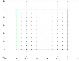
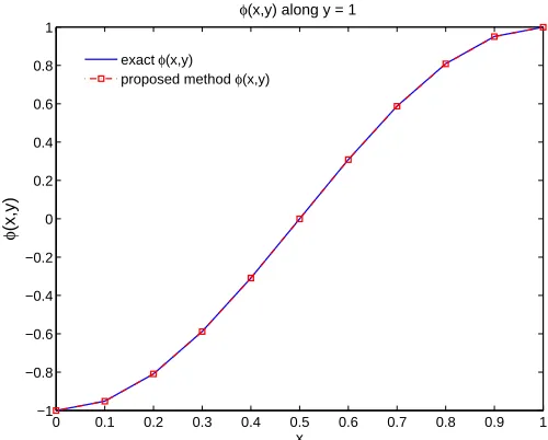
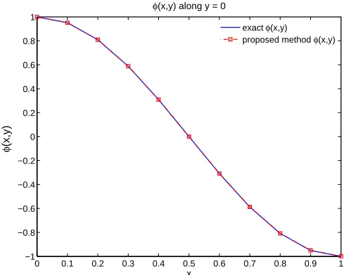
Figure 3 shows the geometry of the problem and the domain discretisation based on a uniform Cartesian grid with 11×11 collocation points (CPs). The obtained results with 11×11 CPs are presented in Figures 4-8. The solution for the primary unknown φ(x, y) on three Neumann boundaries obtained by the present method and the exact solution are plotted in Figures 4-6, the solution for the dual unknownsξ(x, y) (on y = 0 and y = 1) and η(x, y) (on x= 0 and x= 1) are shown in Figure 7 and Figure 8, respectively. From these figures, it can be seen that both the Dirichlet and Neumann boundary conditions are imposed exactly by the present method and the present solutions excellently agree with the exact solutions.
To study the convergence behavior of the solution, a number of uniform grids, namely 11×11, 21×21, 31×31, 41×41, 51×51, 71×71, 81×81, 121×121 and 141×141 CPs is employed in computation. Thehis equivalent to the maximum grid space (inxdirection) for all numerical examples. The convergence behaviours for φ(x, y) (Lφ2) and its derivatives (Lξη2 ) are shown in Figure 9. It can be observed that the errorLφ2 is slightly lower thanLξη2 , the convergence rates for φ(x, y) and (ξ(x, y), η(x, y)) areO(h3.26) andO(h3.5), respectively. At the finest grid, the relative errorLφ2 andL
ξη
−0.2 0 0.2 0.4 0.6 0.8 1 1.2 −0.2
0 0.2 0.4 0.6 0.8 1 1.2
X
[image:12.595.137.471.127.388.2]Y
Figure 3: Poisson equation in regular domains: domain discretisation with 11×11 points.
4.2
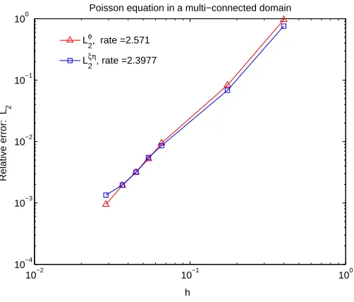
Poisson equation in a multiply-connected domain
To illustrate the proposed interpolation technique for irregular boundaries, we consider the Poisson equation in example 4.1 with a multiply-connected domain as shown in Figure 10, where the Dirichlet boundary condition is prescribed on the left edge and right edge as
φ(−2, y) = cos(πy), (38a)
φ(2, y) = cos(πy), (38b)
and the Neumann boundary condition is given on the other edges: upper edge, lower edge and curve edge as follows
∂φ(x,2)
∂x = 0, (39a)
∂φ(x,−2)
∂y = 0, (39b)
nx
∂φ(x, y) ∂x +ny
∂φ(x, y)
∂y =q(x, y), on x
2+y2= 1, (39c)
wheren(nx, ny) is the outward unit normal to the curve,q(x, y) =−nxπsin(πx) cos(πy)−nyπcos(πx) sin(πy).
0 0.1 0.2 0.3 0.4 0.5 0.6 0.7 0.8 0.9 1 −1
−0.8 −0.6 −0.4 −0.2 0 0.2 0.4 0.6 0.8 1
x
φ
(x,y)
φ(x,y) along y = 1
exact φ(x,y)
[image:13.595.136.386.128.329.2]proposed method φ(x,y)
Figure 4: Poisson equation in regular domain - solution ofφ(x, y) obtained by the proposed method in comparison with exact solution: alongy= 1.
In the case of irregular domains, the irregular boundary interpolation technique in section 3.2 is employed to improve the performance of 1D-IRBFN approximation. Figures 11-13 shows the numerical results by the present method along the curved boundary (Neumman boundary condition). It can be seen that the obtained results are in good agreement with the exact solution. The convergence of the method is investigated with 120, 512, 3232, 4688, 6716, 9984 and 16084 nodes (which are based on uniform grids of 11×11, 24×24, 62×62, 75×75, 90×90, 110×110 and 140×140 nodes) as plotted in Figure 14. The convergence rates for φ(x, y) and its derivatives are O(h2.57) and O(h2.40), respectively. At the finest grid, the relative error Lφ
2 and L
ξη
2 are 9.455×10⁻⁴ and 1.345×10⁻³, respectively. The obtained results indicate that the proposed
boundary interpolation technique greatly improves accuracy of 1D-IRBFN in irregular domains.
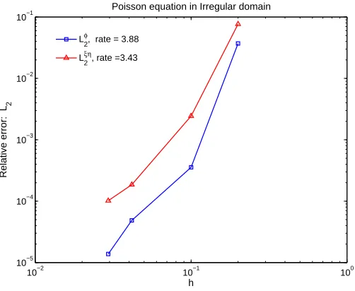
4.3
Poisson equation in irregular domain
The Poisson equation in example 4.1 is examined in a more complicated irregular domain as shown in Figure 15. The Dirichlet boundary conditions on the upper edge and the left edge are given as follows.
φ(0, y) = cos(πy), on x= 0, (40a)
0 0.1 0.2 0.3 0.4 0.5 0.6 0.7 0.8 0.9 1 −1
−0.8 −0.6 −0.4 −0.2 0 0.2 0.4 0.6 0.8 1
x
φ
(x,y)
φ(x,y) along y = 0
exact φ(x,y)
[image:14.595.136.386.128.328.2]proposed method φ(x,y)
Figure 5: Poisson equation in regular domain - solution ofφ(x, y) obtained by the proposed method in comparison with exact solution: alongy= 0 .
The Neumann boundary conditions on the inner arc and the outer arc are, respectively
nx
∂φ(x, y) ∂x +ny
∂φ(x, y)
∂y =q(x, y), on x
2+y2= 1, (41a)
nx
∂φ(x, y) ∂x +ny
∂φ(x, y)
∂y =q(x, y), on x
2+y2= 4, (41b)
whereq(x, y) =−nxπsin(πx) cos(πy)−nyπcos(πx) sin(πy).
The complexity is increased with the Neumann boundary conditions on two curved boundaries. Making use of the proposed boundary interpolation scheme, the irregular boundaries can be ac-curately represented as in the following obtained results. A number of grids of 77, 275, 1459 and 2872 CPs is used for computation. Figure 16 numerically shows the convergence behavior of the method. The convergence rates of the present method for primary variableφand dual variables (ξ, η) areO(h3.88) andO(h3.43), respectively. At the finest grid, the relative errorLφ
2 andL
ξη
2 are 1.375×10⁻⁵ and 1.016×10⁻⁴, respectively.
4.4
Linear elastic cantilever beam
0 0.1 0.2 0.3 0.4 0.5 0.6 0.7 0.8 0.9 1 −1
−0.8 −0.6 −0.4 −0.2 0 0.2 0.4 0.6 0.8 1
y
φ
(x,y)
φ(x,y) along x = 1
exact φ(x,y)
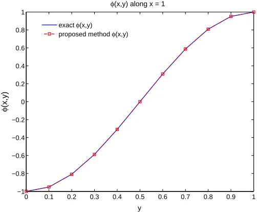
[image:15.595.136.387.150.357.2]proposed method φ(x,y)
Figure 6: Poisson equation in regular domain - solution ofφ(x, y) obtained by the proposed method in comparison with exact solution: alongx= 1.
0 0.1 0.2 0.3 0.4 0.5 0.6 0.7 0.8 0.9 1 0
0.5 1 1.5 2 2.5 3 3.5
x
ξ
(x,y)
ξ(x,y) along y = 1
exact ξ(x,y) proposed method ξ(x,y)
0 0.1 0.2 0.3 0.4 0.5 0.6 0.7 0.8 0.9 1 −3.5
−3 −2.5 −2 −1.5 −1 −0.5 0
x
ξ
(x,y)
ξ(x,y) along y = 0
exact ξ(x,y) proposed method ξ(x,y)
(a) (b)
[image:15.595.143.535.447.619.2]0 0.1 0.2 0.3 0.4 0.5 0.6 0.7 0.8 0.9 1 −3.5
−3 −2.5 −2 −1.5 −1 −0.5 0 0.5
y
η
(x,y)
η(x,y) along x = 0
exact η(x,y) proposed method η(x,y)
0 0.1 0.2 0.3 0.4 0.5 0.6 0.7 0.8 0.9 1 0
0.5 1 1.5 2 2.5 3 3.5
y
η
(x,y)
η(x,y) along x = 1
exact η(x,y) proposed method η(x,y)
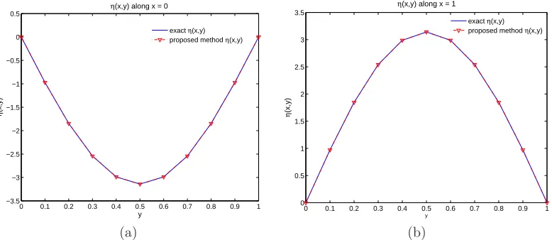
[image:16.595.145.534.156.325.2](a) (b)
Figure 8: Poisson equation in regular domain - solution ofη(x, y) obtained by the proposed method in comparison with exact solution: (a) alongx= 0, (b) alongx= 1.
10−3 10−2 10−1
10−7 10−6 10−5 10−4 10−3 10−2
Relative error: L
2
h
L2φ , rate = 3.26
L2ξη, rate = 3.50
Figure 9: Poisson equation in regular domain: relative errorLφ2 and L
ξη
[image:16.595.136.386.423.618.2]−2 −1.5 −1 −0.5 0 0.5 1 1.5 2 −2
−1.5 −1 −0.5 0 0.5 1 1.5 2
X
Y
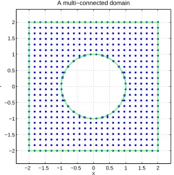
[image:17.595.139.391.138.392.2]A multi−connected domain
Figure 10: Poisson problem in a multiply-connected domain: domain discretisation with 512 nodes.
−4 −3 −2 −1 0 1 2 3 4
−1 −0.8 −0.6 −0.4 −0.2 0 0.2 0.4
θ (rad)
φ
(x,y)
Exact solution Proposed method
[image:17.595.137.368.446.625.2]−4 −3 −2 −1 0 1 2 3 4 −3
−2 −1 0 1 2 3
θ (rad)
ξ
(x,y)
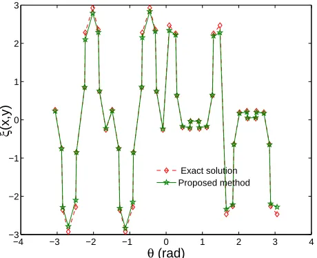
[image:18.595.138.368.144.331.2]Exact solution Proposed method
Figure 12: Poisson equation in a multiply-connected domain: solutions along curved boundary ξ(x, y) with 512 nodes.
−4 −3 −2 −1 0 1 2 3 4
−3 −2 −1 0 1 2 3
θ (rad)
η
(x,y)
Exact solution Proposed method
[image:18.595.139.390.415.614.2]10−2 10−1 100
10−4
10−3
10−2
10−1
100
Relative error: L
2
h
Poisson equation in a multi−connected domain
L2φ, rate =2.571
L
2
[image:19.595.137.388.132.346.2]ξη, rate =2.3977
Figure 14: Poisson equation in a multiply-connected domain: relative errors Lφ2 and Lξη2 and convergence rates.
0 0.5 1 1.5 2
−2 −1.5 −1 −0.5 0
x
y
[image:19.595.140.389.397.639.2]10−2 10−1 100 10−5
10−4 10−3 10−2 10−1
Relative error: L
2
h
Poisson equation in Irregular domain
L2φ, rate = 3.88
L2ξη, rate =3.43
[image:20.595.137.388.160.366.2]Figure 16: Poisson equation in irregular domain: relative errorsLφ2,Lξη2 and convergence rates.
Figure 18: Cantilever beam: discretisation model with 20×5 CPs.
0 0.5 1 1.5 2 2.5 3 3.5 4 4.5 5
−2 0 2 4 6 8
10x 10
−3
x
v(x,y)
exact v proposed method v
[image:21.595.136.347.425.602.2]−0.5 −0.4 −0.3 −0.2 −0.1 0 0.1 0.2 0.3 0.4 0.5 −4
−3.5 −3 −2.5 −2 −1.5 −1 −0.5
0x 10
−5
y
sxy
exact s xy proposed method s
[image:22.595.137.347.162.326.2]xy
Figure 20: Cantilever beam: sxy along Dirichlet boundaryx=L with 20×5 CPs (µ= 0.3).
0 0.5 1 1.5 2 2.5 3 3.5 4 4.5 5 0
1 2 3 4 5 6 7 8x 10
−4
x
sx
exact sx proposed method sx
0 0.5 1 1.5 2 2.5 3 3.5 4 4.5 5 −7
−6 −5 −4 −3 −2 −1 0 1x 10
−4
x
sx
exact sx proposed method sx
(a) (b)
Figure 21: Cantilever Beam (µ= 0.3): sx solution with 20×5 CPs (a) alongy=D/2, (b) along
[image:22.595.145.538.432.606.2]10−2 10−1 100 10−6
10−5 10−4 10−3 10−2 10−1 100
Relative error: L
2
h
Timoshenko Beam: µ = 0.3
Proposed method: L 2
u, rate = 3.1265
Proposed method: L 2
σ, rate = 3.0557
[image:23.595.137.387.286.492.2]FEM: L2u, rate = 1.844
Figure 22: Cantilever beam (µ= 0.3): relative errorsLu
10−2 10−1 100 10−6
10−5 10−4 10−3 10−2
Relative error: L
2
h
Timoshenko Beam: µ = 0.5
Proposed method: L 2
u, rate = 3.1251
Proposed method: L 2
[image:24.595.135.388.127.335.2]σ, rate = 2.9794
Figure 23: Cantilever beam (µ= 0.5): relative errorsLu
2 andLσ2 and convergence rates.
The following parameters are used for the problem: L = 4.8 and D = 1.2. The beam has a unit thickness. Young’s modulus isE = 3×10⁶ , Poisson’s ratio is µ= 0.3 (also µ = 0.5) and the integrated parabolic shear force isP = 100. Plane stress condition is assumed and there is no body force.
The exact solution for this problem was given by Timoshenko and Goodier (1970) as
σxx(x, y) =
P(L−x)y
I (42a)
σyy(x, y) = 0 (42b)
τxy(x, y) =−P
2I
D2 4 −y
2
(42c)
The displacements are given by
ux=
P y 6EI
(6L−3x)x+ (2 +ν)
y2−D2 4
(43)
uy= −P y
6EI
3νy2(L−x) + (4 + 5ν)Dx 2
4 + (3L−x)x 2
(44)
[image:24.595.200.556.442.600.2]The exact displacement (43) and (44) are applied on the Dirichlet boundaryx=L. In the Galerkin formulation, the traction-free boundary condition is automatically met but in a collocation scheme, the the traction-free condition must be explicitly enforced.
Figure 19 shows a comparison of the exact solution and that of the present method (with a regular grid of 5×20 CPs) for the beam deflection uy(x, y) along the x-axis. An excellent
−1 −0.5 0 0.5 1 1.5 2 2.5 3 3.5 4 −5.5
−5 −4.5 −4 −3.5 −3 −2.5 −2 −1.5 −1 −0.5
Log10(CPU time)
Log
10
(error in displacement)
[image:25.595.136.389.127.322.2]proposed method FEM
Figure 24: Cantilever beam (µ= 0.3: comparison of efficiency between the proposed method and FEM. Computational cost (second) versus L2 relative error norm in displacement.
illustrate the comparison between analytically calculated solutions and the numerical results for sxyalongx=Landsxalong upper and lower edges. Again, the plots show that numerical solution
and exact solution are in excellent agreement, which is confirmed by the error measures as shown in Figure 22. The present results compare very favourably with those of Zhang et al [13] and Pan et al [17]. Thus, compared with the standard collocation method, the present method has a good accuracy and stability for this problem.
For the convergence studies, a number of regularly distributed grids of 20×5, 36×9, 52×13, 68×17, 84×21, 124×31 and 164×41 CPs is employed for both compressible material (µ= 0.3) and incommpressible material (µ= 0.5) cases. The convergence behavior in the case of µ= 0.3 are shown in Figure 22, which indicates that the present method has a very good stability and accuracy with a convergence rate of 3.1265 and 3.0557 for displacement and stress, respectively. At the finest grid, the relative errorLu
2 andLσ2 are 5.102×10⁻⁶ and 4.802×10⁻⁶, respectively. Moreover, unlike the displacement-based formulation, in which the accuracy for stress variables is much lower than that for the displacement variables, the proposed method obtained a higher accuracy and convergence rate for the stress field as well.
The robustness of the proposed method in the incompressible limit is also examined. The cantilever beam problem is analyzed with different values of Poisson ratio: µ= 0.499,µ= 0.49999, andµ= 0.5. Our numerical experiments indicate that the volumetric locking can be alleviated by the present approach without any extra effort even in the case ofµ= 0.5, for which the convergence behavior is presented in Figure 23, showing good stability and high accuracy. The convergence rates for displacement and stress variables areO(h3.215) and O(h3.0), respectively. At the finest grid, the relative errorLu
2 andLσ2 are 4.818×10⁻⁶ and 4.869×10⁻⁶, respectively.
−2.3 −2.25 −2.2 −2.15 −2.1 −2.05 −2 −1.95 −1.9 −1.85 −1.8 0.5
0.6 0.7 0.8 0.9 1 1.1 1.2
Log
10(error in displacement)
DCC: Log
10
(CPU time)
[image:26.595.159.447.137.351.2]Proposed method ES−PIM(T3) ES−RPIM(T6)
Figure 25: Cantilever beam (µ = 0.3): comparison of efficiency between the proposed method and the most efficient ES-PIM and ES-RPIM. Differential computational cost (DCC) of different methods in comparison with FEM (CPU time of FEM−CPU time of the reference method) at the same level of relative error in displacement norm.
24 demonstrate that not only the accuracy and order of convergence but also the efficiency of the former exceed those of the latter. Furthermore, the efficiency of the proposed method is compared with that of the latest meshfree method, namely the edge based smooth point interpolation methods (ES-PIM and ES-RPIM) [44], by plotting the differential computational cost (DCC) of the methods in comparison with the FEM (DCC = CPU time of FEM−CPU time of the reference method) at the same level of relative error in displacement norm (Figure 25). It can be observed that the proposed method is less efficient than ES-PIM(T3) (the most efficient one among the ES-PIM family) but more efficient than ES-RPIM(T6) (the most efficient one among the ES-RPIM family).
4.5
Linear elastic infinite plate with a circular hole
In this example, an infinite plate with a circular hole subjected to unidirectional tensile load of 1.0 inxdirection as shown in Figure 26 is analyzed. The radius of the hole is taken as 1 unit. Owing to symmetry, only the upper right quadrant [0,3]×[0,3] of the plate is modeled (Figure 27).
Figure 26: Infinite plate with a circular hole.
σx(x, y) =σ
1−a
2
r2
3
2cos(2θ) + cos(4θ)
+3a 4
2r4 cos(4θ)
, (45a)
σy(x, y) =−σ
a2 r2
1
2cos(2θ)−cos(4θ)
+3a 4
2r4 cos(4θ)
, (45b)
τxy(x, y) =−σ
a2 r2
1
2sin(2θ) + sin(4θ)
−3a
4
2r4sin(4θ)
, (45c)
where (r, θ) are the polar coordinates,athe radius of the hole.
The corresponding displacements, in plane stress case, are given by
ux(x, y) =σ
(1 +µ) E
1
1 +µrcos(θ) + 2 1 +µ
a2
r cos(θ) + 1 2
a2
r cos(3θ)− 1 2
a4
r3cos(3θ)
(46a)
uy(x, y) =σ
(1 +µ) E
−µ
1 +µrsin(θ) + 1−µ 1 +µ
a2
r sin(θ) + 1 2
a2
r sin(3θ)− 1 2
a4 r3sin(3θ)
(46b)
The boundary conditions of the problem are as follows. The tractions which correspond to the exact solution for the infinite plate are applied on the top and right edges, the symmetric conditions are applied on the left and bottom edges, and the edge of the hole is traction free.
The obtained results with 493 CPs are plotted in the Figures 28-29. Figure 28 expresses a comparison of displacementux(x, y) alongy= 0 by the numerical method and the exact solution.
This figure shows that the obtained result is in good agreement with the analytical solution. Figure 29 demonstrates a comparison of stress sx(x, y) a long x= 0 by the proposed method and the
exact solution. An excellent agreement of the numerical stress and the exact one can be observed in this figure.
Figure 27: Infinite plate with a circular hole: domain discretisation with 493 CPs.
curves for a compressible case (µ = 0.3) are presented in Figure 30. A good stability and high accuracy are obtained in this problem as shown in the figure. The same rates of convergence are observed for displacement and stress. The convergence rates for displacement and stress variables are O(h4.141) and O(h4.028), respectively. At the finest grid, the relative error Lu
2 and Lσ2 are 8.687×10⁻⁴ and 6.221×10⁻⁴, respectively.
The above configurations of collocation points are also employed to examined the performance of the present method in the case of incompressible materials (µ= 0.5). The convergence behavior is presented in Figure 31. Like the cantilever beam example, the obtained results indicates that the volumetric locking due to incompressibility is alleviated. A good accuracy and high convergence rate are obtained even in the case of µ= 0.5 as shown in Figure 31. The convergence rates for displacement and stress variables areO(h4.183) andO(h4.118), respectively. At the finest grid, the relative errorLu
2andLσ2 are 1.147×10⁻³and 8.086×10⁻⁴, respectively. Unlike standard collocation method, which is very unstable for elasticity problems with traction boundary conditions [13, 17], the present method shows a superior accuracy and stable convergence.
5
CONCLUSION
This paper reports a successful solution approach for problems governed by high order PDEs where the governing equations are reformulated as first-order systems. Such first-order systems are then numerically modelled with Cartesian grid discretisation and 1D-IRBFN, which is efficient (Cartesian grid) and yields high order accuracy (IRBFN), as illustrated by a variety of test problems with regular as well as irregular domains.
1 1.2 1.4 1.6 1.8 2 2.2 2.4 2.6 2.8 3 2.8
3 3.2 3.4 3.6 3.8
4x 10 −3
x
u(x,y)
[image:29.595.139.389.128.336.2]proposed method u(x,y) exact u(x,y)
Figure 28: Infinite plate with a circular hole: ux(x, y) alongy= 0 with 493 CPs (µ= 0.3).
This work is supported by the Australian Research Council. This support is gratefully acknowl-edged. We would like to thank the referees for their helpful comments.
References
[1] Tran-Cong T. Mai-Duy N. A cartesian-grid collocation method based on radial-basis-function networks for solving PDEs in irregular domains. Numerical Methods for Partial Differential Equations, 23:1192–1210, 2007.
[2] S. Bordas, M. Duflot, and P. Le. A simple error estimator for extended finite elements. Communications In Numerical Methods In Engineering, 24:961–971, 2008.
[3] G. R. Liu. Meshfree methods: moving beyond the finite element method. CRC Press, USA, 2003.
[4] P. Le, T. Rabczuk, and T. Tran-Cong. A Moving Local IRBFN Based Galerkin Meshless Method. International Journal for Numerical Methods in Engineering, 2009. about to be submitted.
[5] T. Belytschko, Y. Y. Lu, and L. Gu. Element-free Galerkin methods. International Journal for Numerical Methods in Engineering, 37:229–256, 1994.
1 1.2 1.4 1.6 1.8 2 2.2 2.4 2.6 2.8 3 1
1.5 2 2.5 3 3.5x 10
−3
y sx
[image:30.595.139.388.126.332.2]proposed method sx exact sx
Figure 29: Infinite plate with a circular hole: sxalongx= 0 with 493 CPs (µ= 0.3).
[7] P. Le, N. Mai-Duy, T. Tran-Cong, and G. Baker. Meshless IRBF-based numerical simulation of dynamic strain localization in quasi-britle materials. In 9th U.S. National Congress on Computation Mechanics, San Francisco, USA, July 2007. CD page 63.
[8] P. Le, N. Mai-Duy, T. Tran-Cong, and G. Baker. An IRBFN Cartesian grid method based on displacement-stress formulation for 2D Elasticity problems. In 8th World congress on Computational Mecanics (WCCM8), Venice, Italy, June–July 2008.
[9] P. Le, T. Rabczuk, N. Mai-Duy, and T. Tran-Cong. A Moving Local IRBFN Based Integration-Free Meshless Method. International Journal for Numerical Methods in Engineering, 2009. about to be submitted.
[10] G. R. Liu and Y. T. Gu. An introduction to Meshfree methods and their programming. Springer, The Netherlands, 2005.
[11] X. Zhang, K. Z. Song, M. W. Lu, and X. Liu. Meshless method based on collocation with radial basis functions. Computational Mechancis, 26:333–343, 2000.
[12] H. Li, T. Y. Ng, J. Q. Cheng, and K. Y. Lam. Hermite -cloud: a novel true meshless method. Computational Mechancis, 33:30–41, 2003.
[13] X. Zhang, X. H. Liu, K. Z. Song, and M. W. Lu. Least-squares collocation meshless method. International Journal for Numerical Methods in Engineering, 51:1089–1100, 2001.
10−2 10−1 100 10−4
10−3 10−2 10−1 100
Relative error: L
2
h
L 2
u, rate = 4.141
L 2
[image:31.595.137.387.126.326.2]σ, rate =4.028
Figure 30: Infinite plate with a circular hole (µ = 0.3): relative error Lu
2, Lσ2 and convergence rates.
[15] G. R. Liu and Y. T. Gu. A meshfree method: Weak-Strong (MWS) form method, for 2D solids. Computational Mechanics, 33:2–14, 2003.
[16] Y. T. Gu and G. R. Liu. A meshfree Weak-Strong (MWS) form method for time dependent problems. Computational Mechanics, 35:134–145, 2005.
[17] X. F. Pan, X. Zhang, and M. W. Lu. Meshless Galerkin least-squares method. Computational Mechancis, 35:182–189, 2005.
[18] H.Y. Hu, J.S. Chen, and W. Hu. Weighted radial basis collocation method for boundary value problems. International Journal for Numerical Methods in Engineering, 69:2736–2755, 2006.
[19] J.S. Chen, W. Hu, and H.Y. Hu. Reproducing kernel enhanced radial basis collocation method. International Journal for Numerical Methods in Engineering, 75:600–627, 2008.
[20] S. N. Atluri, Z. D. Han, and A. M. Rajendran. A New Implementation of the Meshless Finite Volume Method, Through the MLPG “Mixed” Approach. CMES: Computer Modeling in Engineering & Sciences, 6(6):491–513, 2004.
[21] S. N. Atluri, H. T. Liu, and Z. D. Han. Meshless local petrov-galerkin (MLPG) mixed colloca-tion method for elasticity problems. CMES: Computer Modeling in Engineering & Sciences, 14(3):141–152, 2006.
10−2 10−1 100 10−4
10−3 10−2 10−1 100
Relative error: L
2
h
L2u, rate = 4.183
[image:32.595.137.388.126.329.2]L2σ, rate =4.118
Figure 31: Infinite plate with a circular hole (µ = 0.5): relative error Lu
2, Lσ2 and convergence rates.
[23] S.H. Lee and Y.C. Yoon. Meshfree point collocation method for elasticity and crack problems. International Journal for Numerical Methods in Engineering, 61:22–48, 2004.
[24] Z. Cai, R. D. Lazarov, T. Manteuffel, and S. McCormick. First order system least-square for second-order partial differential equations: Part 1. SIAM J. Numer. Anal., 31:1785–1799, 1994.
[25] Z. Cai, T. Manteuffel, and S. McCormick. First order system least-squares for second-order partial differential equations: Part 2. SIAM J. Numer. Anal., 34:425–454, 1997.
[26] Z. Cai, T. Manteuffel, and S. McCormick. First order system least-squares for stokes equations with application to linear elasticity. SIAM J. Numer. Anal., 34:1727–1741, 1997.
[27] Z. Cai, T. Manteuffel, S. McCormick, and S. Parter. First order system least-squares (FOSLS) for planar linear elasticity: pure traction problem. SIAM J. Numer. Anal., 35:320–335, 1998.
[28] Z. Cai, C.-O. Lee, T. Manteuffel, and S. McCormick. First order system least-squares for linear elasticity: numerical results. SIAM J. SCI. COMPUT., 21:1706–1727, 2000.
[29] Z. Cai and G. Starke. First order system least-squares for stress-displacement formulation linear elasticity. SIAM J. Numer. Anal., 41:715–730, 2003.
[30] B. Lee. First order system least-squares for elliptic problems with Robin boundary conditions. SIAM J. Numer. Anal., 37:70–104, 1999.
[32] S. Park and S. Youn. The least-squares meshfree method.International Journal for Numerical Methods in Engineering, 52:997–1012, 2001.
[33] K. Kwon, S. Park, B. Jiang, and S. Youn. The least-squares meshfree method for soving linear elastic problems. Computational Mecchanics, 30:196–211, 2003.
[34] P. J. Roache. Computational Fluid Dynamics. Hermosa Publisher, 1980.
[35] P. Le, N. Mai-Duy, T. Tran-Cong, and G. Baker. A numerical study of strain localization in elasto-therno-viscoplastic materials using radial basis function networks. CMC: Computers, Materials & Continua, 5:129–150, 2007.
[36] P. Le, N. Mai-Duy, T. Tran-Cong, and G. Baker. A meshless modeling of dynamic strain localization in quasi-britle materials using radial basis function networks. CMES: Computer Modeling in Engineering & Sciences, 25(1):43–66, 2008.
[37] J. Dolbow and T. Belytschko. Volumetric locking in the element-free Galerkin method. In-ternational Journal for Numerical Methods in Engineering, 46:925–942, 1999.
[38] J.S. Chen, HP. Wang, S. Yoon, and Y. You. An improve reproducing kernel particle methods for nearly incompressible finite elasticity. Comp. Meth. Appl. Mech. Eng., 181:117–145, 2000.
[39] W.R. Madych. Miscellaneous error bounds for multiquadric and related interpolators.Compu. Math. Appl., 24:121–138, 1992.
[40] N. Mai-Duy and T. Tran-Cong. Numerical solution of differential equations using multiquadric radial basic function networks. Neural Networks, 14:185–199, 2001.
[41] N. Mai-Duy and T. Tran-Cong. Approximation of function and its derivatives using radial basis function networks. Applied Mathematical Modeling, 27:197–220, 2003.
[42] N. Mai-Duy and T. Tran-Cong. An efficient indirect RBFN-based method for numerical solution of PDEs. Numerical Methods for Partial Differetial Equations, 21:770–790, 2005.
[43] J. Wertz, E.J. Kansa, and L. Ling. The role of the multiquadric shape parameters in solving elliptic partial differential equations.Computers and Mathematics with Applications, 51:1335– 1348, 2006.