Matching and fusing signal-estimation errors for similarity-based pattern classification

Matching and Fusing Signal-Estimation Errors for

Similarity-based Pattern Classification

TUAN D. PHAMt.:t

tBioinfonnatics Applications Research Centre +School of Mathematics, Physics, and Infonnation Technology

James Cook University Townsville, QLD 481 I

AUSTRALIA [email protected]

Abstract: Error estimation using different optimal models for signal processing has been an active research field in data

analysis such as speech recognition, image analysis, geophysics, and earth science. A popular direction of research in pattern classification is to develop computational models for comparing objects being either abstract or physical based on some measure of similarity or dissimilarity. This paper explores some linear-prediction models for deriving signal estimation errors and their fusion for similarity-based pattern classification.

Key-Words: Linear prediction, error matching, similarity measure, infonnation fusion, classification.

1 Introduction

A basic study in the broad field of pattern recognition is the selection of good features that can be effectively utilized to distinguish the identities of different objects. Typically, sufficient collection of these features are used to train clas-sifiers that are supervised to be able to classifY unknown objects based on past learning. However, there are many practical pattern-recognition problems where the availabil-ity or the sufficient amount of good features are not feasible for machine-learning purpose. These are cases when the object features involve with high dimensionalities or the datasets are limited. An alternative strategy is to classifY patterns based on some measures of similarity or dissimi-larity between the two objects. Tliis type of approach has recenly renewed and regained increased attention among the community of pattern-recognition researchers [I].

Metric-based measures of similarity have been conven-tionally applied for the design of various machine-learning methods. An alternative representation of similarity or dis-similarity is the the notion of non-metric measure known as the distortion measure which relaxes the symmetrical prop-erty of the distance measure. The central idea of a distor-tion measure is based on the error matching of the estima-tions of the two signals. This type of measure has been particularly explored and applied for solving problems in speech recognition. Its various fonns are based on the the theory of linear predictive coding and still remain an im-portant research area of digital signal processing for signal detection and signal coding [2, 3, 4, 5].

LPC has become a popular signal processing tool be-cause 1) it is very useful for low-bit-rate coding, 2) it

pro-vides a compact and tractable presentation of the spectral properties of the signals, and 3) its computation is relatively simple. Given its advantages, the theory of LPC has not widely applied for the analysis of other types of data such as modem biomedical and biological signals including ge-nomic, proteomic, and microarray data [6,7,8,9, 10, i24]. In addition, the fonnulation ofthe LPC and LPC-based dis-tortion measures have not been well explored to capture the spatial infonnation which inherently exists in several do-mains of real data including those having described before. Besides the exploration of various sources of information for measuring similarities between objects for pattern clas-sification, it is beneficial to take advantage of these sources by integrating the independent pieces of evidence in order to improve the recognition rate instead of solving the prob-lem separately with different measures.

2 Linear Predictive Coding

In time series analysis, a continuous-time signal s(t) is sampled to obtain a discrete-time signal s(nT), where n

is an integer variable and T is the sampling interval. For the sake of convenience, from now on we denote s(nT) as

s( n) without the loss of generality.

The basic formulation oflinear prediction is based on the assumption that a signal Sn is considered to be the out-put of some sytem with some unknown inout-put Un such that [2]

p q

Sn

=

I>ks(n - k)

+

G2:)lu(n -l) (1)

k=l 1=0

where bo

=

1, the terms {ak} and the gain G are the pa-rameters of the hypothesized system.

Equation (I) can be expressed in the frequency domain by taking the z transform on its both sides, which results in

H(z) = S(z)

=

G 1

+

~i-l

_b1z-lk

U(z) 1

+

I:k=l

akZ- (2)

where H (z) is the system transfer function, U (z) is the z

transform ofu(n), and S(z) the z transform of s(n) which is defined as

co

S(z) =

:L

s(n)z-n (3) n=-oo

The term H(z) expressed in (2) is called the general

pole-zero model- the roots of the numerator are the zeros,

and the roots of the denominator are the poles of the model.

Thus, two special cases of the model are the all-zero and all-pole models. As the names refer, for the all-zero model:

ak

=

0, Vk; whereas for the all-pole model: bl

=

0, Vl.

Our discussion is now focused on theall-pole model which assumes that the signal s(n) can be determined as a linear combination of the past values and some input u(n):

p

s(n) =

:L

aks(n - k)

+

Gu(n) (4)

k=l

where G is a gain factor and the transfer function

H

(z) of the all-pole model simplyfies to

G

H(z) = P k

1

+ I:k=l

akZ

-(5)

In general, the problem of the linear prediction based on the all-pole model is to determine the set of the predictor coefficients {ak} and the gain G. In many applications the input u( n) is unknown. This fact further reduces the linear prediction model to

P

s(n)

=

:L

ak s(n - k) (6)

k=l

where s(n) is the approximation of s(n).

The prediction error e( n) between the observed sample

s(n) and the predicted value s(n) can be defined as

P

e(n)

=

s(n) - s(n)

=

s(n) -

:L

ak s(n - k) (7) k=l

Since the spectral properties of the signal can vary over time, the predictor coefficients at a given time n must be es-timated from a short segment of the signal occuring around time n. Using the principle of least squares, we can find an optimal set of predictor coefficients by minimizing the mean-squared prediction error over a short segment of the whole signal.

A short-term signal, sn(m), and its error segment,

en(m), at time n can be defined as

sn(m) = s(n

+

m) (8)

and

en(m) = e(n

+

m) (9)

The mean-squared error signal at time n to be

mini-mized is defined as

(10)

m

which can be expressed in terms of s n (m) as follows.

Differentiating En, which is expressed in (11), with respect to each ak and set the result to zero:

giving

BEn

-;:;-- = 0, k = 1, ... ,p

Uak

P ,

(12)

:L

sn(m - i)sn(m) =

2:

ak

L:

Sn(m - i)sn(m - k)

m k=l m

(13) It can be noticed that the terms of the form

I:

sn(m-i)sn (m - k) are those of the short-term covariance of

sn(m), that is

m

signal s(m

+

n) is multiplied by a finite length window,

w(m), which zero outside the range 0 :S m ::; N -1. Thus the segment for minimization can be expressed as

( ) _ { s(m

+

n) w(m) : O:S m ::; N - 1

Sn m - 0 : otherwise

(15) where w (m) is usually a Hamming window.

Based on using the signal expressed in (15), the error signal en(m) is exactly zero since sn(m) = 0 for all m

<

0, and for m

>

N - 1

+

P the prediction error is also zero because again sn(m)

=

0 for all m

>

N - 1. Thus an optimal range of m used in defining the short segment of

the sequence and the region over which the mean-squared error is ~inimized is from m

=

0 to m

=

N - 1

+

P to minimize the errors at section boundaries. Using this range for m, the mean-squared error becomes [3]

N-l+p

En

=

L

e;'(m) (16)

m=O

and rPn

(i,

k) can be rewritten as

N-l+p

rPn(i, k)

=

L

sn(m-i)sn(m-k),l::; i ::; p, 0::; k ::; p

m=O

(17) or

equal), r is a p x 1 autocorrelation vector, and a is a p x 1 vector of prediction coefficients:

r

~:~~~

R

=

Tn(2) Tn(P - 1)

and

Tn(1) Tn(2) Tn(O) Tn(l) Tn

(1)

Tn(O)

Tn(P-1) Tn(P - 2)

Tn(p-3)

Tn(O)

Thus, the LPC coefficients can be obtained by solving

(22)

3 Spatial Linear Predictive Coding

Having outlined the theory of linear predictive coding (LPC), we present in this section a new approach for es-timating the LPC model parameters based on the theory of regionalized variables [11] and the kriging estimation pro-cedure [12, 13]. A regionalozed variable is thought to have characteristics intermediate between a random variable and a deterministic function - its values vary over space but are spatially correlated over some short distance. The degree of the spatial continuity of a regionalized variable can be

. expressed by a semivariogram (to be discussed later). We

N-l-(,-k) d 'b h h h f ' I' d . bl d

.

L

.

k . k now escn e ow t e t eory 0 regIOna lze vana es an A--n(z k)

=

sn(m)sn(m+z- ,), 1

<

t

<

p,O

< <

P h b' d . . fkri' b de

'P , - - - - t e un lase estimatIOn 0 gmg can e use lor

model-m=O

(18) ing the all-pole linear prediction.

Since (18) is a function of (i - k), the covariance func- Consider a stationary random function that consists of tion rPn(i, k) can be reduced to the simple autocorrelation several random variables, one for each of the available

val-function: ues and one for the unknown value. Let V (s( n - k)), k =

N-l-(i-k)

rPn(i, k)

= Tn(i - k)

=

L

sn(m)Sn(m

+

i - k)

m=O

(19) Since the autocorrelation function is symmetric, that is Tn(-k) = Tn(k), the system ofLPC equations can be expressed as

p

LTn(li - kl)ak

= Tn(i),

1 ::; i ::; P (20)

k=l

which describes a set of p equations in p unknowns, and can be expressed in matrix form as

Ra=r (21)

where R is a p x p autocorrelation matrix (Toeplitz ma-trix which is symmetric with all diagonal elements being

1, ... ,p, be the random variables of s(n - k), k = 1, .. . p, respectively. Let V(s(n)) be the random variable for s(n).

These random variables are assumed to have the same prob-ability distribution, and the expected value of the random variables at all locations is E{V}. Thus, the estimate of s (n) is also a random variable and expressed by a weighted linear combination ofthe random variables at p locations:

p

V(s(n)) =

L

ak V(s(n - k))

k=l

And the error of estimation is

R(s(n)) = V(s(n)) - V(s(n))

Altematively we have

p

R(s(n)) =

L

ak V(s(n - k)) - V(s(n)) k=l

(23)

(24)

The expected value of the error of estimate is

p

E{R(s(n))} = L akE{V(s(n - k))} - E{V(s(n))}

k=l

(26) Based on the assumption that the random function is stationary, both E{V(s(n - k))} and E{V(s(n))} can be expressed as E{V}; thus (26) becomes

p

E{R(s(n))}

=

LakE{V} - E{V} (27)

k=l

If the unbiased condition is imposed, then

E{R(s(n))} must be set to zero. Giving

p

E{V} L ak

= E{V}

(28)

k=l

resulting

(29)

k=l

The variance of the random variable V(s(n)) which is the result of a weighted linear combination of other p

random variables is given by

p p p

Vur{L Uk V(s(n-k»} = L L UkUjCov{V(s(n-k»V(s(n-j»}

k=l k=l j=l

(30)

Recalling that R(s(n)) = V(s(n)) - V(s(n)) and us-ing (30), the variance of the error can be expressed as either

Var{R(s(n»} Cov{V(s(n»V(s(n» - 2Cov{V(s(n»V(s(n»}

+ Cov{V(s(n»V(s(n»)} (31)

or

p p p

O"~

=

0"2

+

L L akajCkj - 2 L akCk (32)

k=lj=l k=l

which defines the variance of error as a function of al, ... ,ap .

An optimal choice for the predictor parameters aI, ... , ap is to minimize O"~. Introducing a Lagrange

mul-tiplier (3 into (32) we have

p p p p

(J~

= (J2+ L L a k a j C k j - 2 LakCk+2(3(Lak-l)

k=l j=l k=l k=l

(33) The error variance term, (J~, can now be minimized by differentiating (33) with respect to the predictor coeffi-cients and the Lagrange parameter, and setting each one to zero. By doing so, we obtain the following equations.

p

LajCkj

+

(3 = Ckn, V'k = 1, ... ,po

j=l

p

L

a k=l k=l

(34)

(35)

The above system of equations are known as the ordi-nary kriging system [], which can be expressed in matrix notation as

Ca=D (36)

where

C

l l

C

1p 1

C=

C

pl Cpp 1

1 1 0

a

=

[ak . . . ap (3

1

T

Thus the values of the spatial predictor coefficients can be obtained by solving

a= C-l _{D (37)}

The sample covariance used for the kriging estimator can be calculated as

l I n

C(h)

=

N(h) .. L s(j) - (; Ls(k))2 (38)

(t,J)\hij=h k=l

in which the sample covariance is a function of the lag dis-tance h, N(h) is the number of pairs that s(i) and s(j) are separated by h, and n is the total number of data.

On the derivation of the error of variance, it is assumed that the random variables have the same mean and variance which lead to the development of the mathematical rela-tionship between the variogram, denoted as ,/(h), and the covariance [13]

,/(h)

=

0"2 - C(h) (39) where the sample ,/( h) is defined as

1

,/(h) = 2N(h)

L

[s(i) - s(jW (40)

(i,j)\hij=h

and

p

Lak')'jk -

f3

=

"'{jn, j

=

1, ... ,p

k=l

p

"2::

ak=1

k=l

(41)

(42)

The variance of the estimation residual (error) can readily be determined by

(43) Taking the square root of (43) gives the standard error of the estimate:

(44)

4 Classification by Error Matching

and Fusion

To apply the results obtained from the linear prediction for classification of unknown signals, the method of vec-tor quantization can be utilized to generate a decision logic for classification. We discuss herein the implementation of both conventional and spatial distortion measures and the fusion of the two measures for the VQ-codebook design.

A distortion measure between two vectors x and y, de-noted as D(x, y), is considered to be a cost of reproducing any input vector x as a reproduction of vector y. Given such a distortion measure, the mismatch between two sig-nals can be quantified by an average distortion between the input and the final reproduction. Intuitively, a match of the two patterns is good if the average distortion is small.

A popular distortion measure is the likelihood ratio (LR) distortion. The LR distortion measure, D LR, is de-fined by [3)

a'TRs a'

D LR = aT Rs a - I (45) where Rs is the autocorrelation matrix of signal s associ-ated with its LPC coefficient vector a, and a' is the LPC coefficient vector of signal

s'.

Based on the same principle derived for the likelihood ratio distortion and using (43), the spatial distortion, de-noted as D

s,

can be defined as

aTD

Ds

=

a,TD - 1 (46)

where a defined in (36) is the spatial LPC vector of signal s, D is the matrix defined in (36) associated with s , and a' is the spatial LPC vector of signal

s'.

Based on the two different distortion measures, we can combine them in two simple ways by either summing or

multiplying the two measures in a similar fashion proposed in [14] as follows.

DSum

= DLR

+

Ds (47) or

DProd = DLR X Ds (48)

It is noted that the above two distortion measures are dimensionless. The rationale for taking the sum of the two measures is that if the two features are independent then adding the values of the two measures provides more in-formation for decision making. Whereas the rationale for combining the two measures by the multiplication rule re-lates to the joint probability of the occurrence of the two events. We next discuss how to implement the quantiza-tion ofthe LPC vectors of coefficients and limit the case to one-dimensional signal.

Now assume we have a set of T frames or sub-sequences of the whole signal, which are represented by the corresponding set of T LPC vectors A {al,a2, ... ,aT},whereat

=

(atl,at2, ... ,atp). It can be seen that these LPC vectors represent a type of feature of the sequence. Let the codebook of the LPC vectors be

e

= {Cll C2,· .. , CN}, where Cn = (Cnll Cn 2,· ..

,Cnp),

n

=

1,2, ... , N are codewords. Each codeword Cn is

assigned to an encoding region Rn in the partition

n

=

{Rl' R2 , . .. , RN}. The source LPC vector at can be

reP-resented by the encoding region Rn and expressed by (49) The main idea ofLPC based vector quantization (VQ) is to find an optimal codebook such that for a given train-ing set A and a codebook size N, the average distortion in representing each LPC vector at by the closest codeword

Cn is minimum. In mathematical terms we express

D*

=

min

[-Tl

t

min

(D(Cn,at))]

en t=l 15,n5,N

(50)

where D is an LPC distortion (either DLR, Ds, D Aver,

or D Prod), and D* is the average distortion of the vector quantizer.

Table 1: k-fold cross validation results for ovarian cancer data (/Lcl: control mean, /Ler: cancer mean)

SVM DLR/Ds Dsum/Dprod

k /Lcl /Ler /Lcl

2 0.8930 0.9492 0.9224/0.9231 4 0.9058 0.9722 0.9327/0.9320

6 0.9094 0.9760 0.9348/0.9332 8 0.9098 0.9784 0.9362/0.9359

10 0.9096 0.9801 0.937710.9412

and iteratively bi-partitions the codevectors based on the optimality criteria of nearest-neighbor and centroid condi-tions until the number of codevectors is reached.

The classification system based on the LPC analysis and VQ codebook approach works as follows. The given input signal is analyzed by the LPC giving the sequence of LPC vectors. The resultant LPC vectors are quantized using the number of codebooks according to the number of different classes. The distortions with respect to each code book are accumulated across the whole test. The aver-age spectral distortion (dissimilarity) measure between an unknown sample and a particular known class is

(51 )

where D is a spectral distortion measure, D is the average distortion, Xm is an LPC vector of the unknown signal, T

is the number of LPC vectors of the unknown signal,

c}

is the j LPC-VQ codevector of a particular class represented by codebook Ci , and J the size of Ci .

The unknown signal is assigned to class i * if the av-erage distortion measure of its LPC feature vector Xm and the LPC feature codebook Ci _{is minimum, that is}

i* = argrninD(xm,

,

Ci ) (52)

5 Application

The identification of biomarkers using mass spectrometry (MS) data is a challenging task which requires the combi-nation of the contrast fields of knowledge of modem biol-ogy, signal processing, and pattern recognition. The basic problem is to classify an unknown MS signal as either the control (non-disease) group or the disease group. Figure 1 illustrates the classification system based on the LPC anal-ysis and VQ codebook approach.

The proposed method (spatial LPC-VQ) was tested using a public ovarian high-resolution SELDI-TOF mass spectrometry dataset. Regarding the implementation of proposed method, the number of poles p = 8 was speci-fied for the LPC analysis. The codebook size of 64

code-/Ler /Lcl /Ler

0.9637/0.9640 0.923110.9245 0.9643/0.9641

0.981110.9821 0.933010.9326 0.9832/0.9829

0.9825/0.9814 0.9352/0.9337 0.9842/0.9828

0.9852/0.9887 0.937810.9362 0.9859/0.9889

0.9885/0.9890 0.9388/0.9434 0.9892/0.9891

VnknO\\11 :viS ~igllal

: compans:ons

[image:6.597.132.489.122.202.2]

Clil.5sificati..-m .nfunbl0Wi1 i\{S sig.na1

Figure I: LPC-VQ-based MS-data classification system

80

70 60

2>

.~ 50

~

40 30

20 10

o~----~--~~----~----~----~

-5000 5000 10000 15000 20000

mlz

[image:6.597.366.553.315.389.2] [image:6.597.337.524.508.657.2]

100 90 80 70 60

~

~ 50

~

40

30

20 10 0

-5000 sooo 10000 15000 20000

mlz

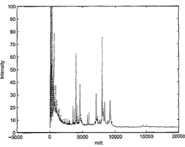
Figure 3: MS-based ovarian cancer data

vectors was used to generate the prototype for the control and cancer classes. Each MS sequence was split into mul-tiple frames of 150 data points having 20 points overlap-ping between the two adjacent frames. At present, these paramters for signal processing were arbitrarily chosen and based on the experience that these values have been con-sidered reasonable for the classification of speech signals. These paramters were also used for the conventional (non-spatial) LPC-VQ method. Figures 2-3 show the typical MS signals of ovarian control, and ovarian cancer respectively. The ovarian high-resolution SELDI-TOF mass spectrometry dataset, which can be obtained from the FDA-NCI Clinical Proteomics Program Databank (http://home.ccr.cancer.gov/ncifdaproteomics/ppattems.asp ), was used to test the proposed spatial LPC-VQ based method. The dataset was generated using a nOFl-randomized study set of ovarian cancers and control specimens on an ABI Qstar fitted with a SELDI-TOF source to study ovarian cancer case versus high-risk control. The dataset consists of 100 control samples and 170 cancer samples. The validation of the classification of the proposed approach was designed with similar strategies to those carried out in [23], who applied support vector q machine (SVM) for the classification, so that comparisons can be made. The measure of performance is the k-fold cross validation where k

=

2, 4, 8, and 10, and each k-fold validation was carried out 1000 times.

It is noted that the raw ovarian high-resolution SELDI-TOF dataset used by Yu et al. [23] consists of 95 con-trol samples and 121 cancer samples; while the raw ovarian high-resolution SELDI-TOF dataset we used to test the per-formance of the proposed approach has 100 control sam-ples and 170 cancer samsam-ples.

Table 1 shows the mean classification values of the

k-fold cross validation obtained from the SVM classification on the preprocessed data and the proposed method using

D LR, D

s,

D Sum, and D Prod. The overall results obtained

for the different types of validation ofthe classification per-formance show that both the spatial and non-spatial LPC-VQ methods are more favorable for MS-based ovarian cancer identification than the other approach in two folds -feature extraction and classification methods. The spatial distortion Ds and the likelihood-ratio distortion D LR are competitive and can be complementary for information fu-sion as shown from the improved classification rates using the two combined measures D Sum and D Prod.

In terms of feature extraction, the procedure for ex-tracting the LPC-based features is more straightforward than the other feature extraction method [23] which trans-forms raw MS data to binned MS data, from binned MS data to Kolmogorov-Smimov(KS)-test based feature selec-tion, from KS-test based features to the restriction of coef-ficient of variation (CV), and finally from the restriction of CV to wavelet coefficients. In terms of pattern classifica-tion, the classification using the VQ-based decision rule is much simpler than the SVM-based classifier; however it is not meant that the SVM-based classifier is inferior to the VQ-based decision rule for classifying MS data. The LPC-based coefficients can be used as robust features for train-ing different classifiers to improve the performance capable of more effective discrimination of complex patterns.

6 Conclusion

We have presented several distortion measures in terms of the matching of signal-estimation errors and their fusion for similarity-based pattern classification. Particularly, we have ciscussed a new implementaion for estimating the spatial linear-predicion coefficients using the principles of the theory of regionalized variables and the unbiased krig-ing estimator. Based on the spatial LPC vectors and the error variance of kriging estimation, we derived a novel spatial distortion measure. We then used two simple strate-gies for the fusion of the two measures to determine the optimal codevectors to serve as a basis a decision logic. In-formation fusion is a an important and interesting topic for signal detection and classification and worth further inves-tigation. We employed a VQ method to model class pro-totypes. However, in case of limited data for training, the decision logic for class assignment can be directly based on the minimum of the distortion between known and un-known classes.

[image:7.595.69.256.109.258.2]

References:

[1] Special Issue: Similarity-based Pattern Recognition, M. Bicego, V Murino, M. Pelillo, and A. Torsello (Eds.), Pattern Recognition, 39: 10 (2006).

[2] J. Makhoul, Linear prediction: a tutorial review, Proc. IEEE, 63 (1975) 561-580.

[3] L. Rabiner, and B.H. Juang, Fundamentals of Speech Recognition. New Jersey, Prentice Hall, 1993.

[4] Ingle, V.K., and Proakis, J.G., Digital Signal Process-ing UsProcess-ing Matlah VA. Boston, PWS PublishProcess-ing, 1997.

T.D. Pham and M. Wagner, A geostatistical model for linear prediction analysis of speech, Pattern Recogni-tion, 31 (1998) 1981-1991.

)] A.K. Whitchurch, Gene expression micro arrays,

IEEE Potentials, 21 (2002) 30-34.

[7] X.Y Zhang, F. Chen, Y.T. Zhang, S.G. Agner, M. Akay, Z.H. Lu, M.M.Y. Waye, and S.K.w. Tsui, Sig-nal processing techniques in genomic engineering,

Proceedings of the IEEE, 90 (2002) 1822-1833.

[8] R. Aebersold, and M. Mann, Mass spectrometry-based proteomics, Nature, 422 (2003) 198-207.

'[9] P. P. Vaidyanathan, Genomics and proteomics: A sig-nal processor's tour, IEEE Circuits and Systems Mag-azine, Fourth Quarter (2004) 6-29.

[10] T.D. Pham, C. Wells, and D.L Crane, Analysis ofmi-croarray gene expression data, Current Bioinformat-ics, 1 (2006) 37-53.

[11] G. Matheron, La theorie des variables regionalisees at ses appplications, Cahier du Centre de Morphologie Mathematique de Fontainebleau. Ecole des Mines,

Paris, 1970.

[12] A.G. Journel, and C.J. Huibregts, Mining Geostatis-tics. Academic Press, London, 1978.

[13] E.H. Isaaks, and R.M. Srivastava, An Introduction to Applied Geostatistics. Oxford University Press, New

York, 1989.

[14] L.R. Rabiner, and M.R. Sambur, Application of an LPC distance measure to the voiced-unvoiced-silence detection problem, IEEE Trans. Acoustics, Speech, and Signal Processing, 25 (1977) 338-343.

[15] R.M. Gray, Vector quantization, IEEE ASSP Mag., 1

(1984) 4-29.

[16] Rabiner, L.R., Sondhi M.M., and Levinson, S.E., A vector quantizer incorporating both LPC shape and energy, Proc. 1984 Int. Conf. Acoustics, Speech, and Signal Processing, pp. 17.1.1-17.1.4, 1984.

[17] Linde, Y., Buzo, A., and Gray, R.M., An Algorithm for Vector Quantization", IEEE Trans. Communica-tions, 28 (1980) 84-95.

[18] E. Sauter et al., Proteomic analysis of nipple aspirate

fluid to detect biologic markers of breast cancer, Br. J Cancer, 86 (2002) 1440-1443.

[19] E.F. Petricoin et al., Use of proteomic patterns in

serum to identifY ovarian cancer, Lancet, 359 (2002)

572-577.

[20] T.P. Conrads, M. Zhou, E.F. Petricoin III, L. Liotta, and T.D. Veenstra, Cancer diagnosis using proteomic patterns, Expert Rev. Mol. Diagn., 3 (2003) 411-420.

[21] E.F. Petricoin, and L.A. Liotta, Mass spectrometry-based diagnostics: The upcoming revolution in dis-ease detection, Clinical Chemist/y, 49 (2003)

533-534.

[22] J.D. Wulfkuhle, L.A. Liotta, and E.F. Petricoin, Pro-teomic applications for the early detection of cancer,

Nature, 3 (2003) 267-275.

[23] J.S. Yu, S. Ongarello, R. Fiedler,

X.w.

Chen, G. Toffolo, C. Cobelli, and Z. Trajanoski, Ovarian can-cer identification based on dimensionality reduction for high-throughput mass spectrometry data,

Bioin-formatics, 21 (2005) 2200-2209.

[24] T.D. Pham, LPC cepstral distortion measure for pro-tein sequence comparison, IEEE Trans. NanoBio-science, 5 (2006) 83-88.

[25] J. Ruiz-Alzola, C. Alberola-Lopez, C.F. Westin, Krig-ing filters for multidimensional signal processKrig-ing,