The use of HF radar surface currents for computing Lagrangian trajectories: benefits and issues

The use of HF radar surface currents for computing

Lagrangian trajectories: benefits and issues

A. Mantovanelli, M. L. Heron, A. Prytz

James Cook University Townsville, QLD 4811, Australia

Abstract- Surface coastal currents mapped by a pair of high frequency ground-wave radars (HFR) have been used to predict Lagrangian trajectories in the proximity of Heron Island (Capricorn Bunker Group, Great Barrier Reef, Australia), and to compare with the current data measured by an Acoustic Doppler Current Profiler (ADCP) at three mooring stations. Overall the HRF and ADCP absolute current speeds showed a difference less than ±0.15 m s-1 for 68% of the observations. A good agreement between HFR (at a depth of 1.5 m) and ADCP (at a depth of 5.5 m) data were observed for the u-component (cross-shelf) which presented a stronger tidal signal, while a poor comparison was found for the v-component (north-south) more influenced by the south-easterly and northerly winds. The HFR allowed inclusion of not only the temporal, but also the spatial current variability in the tracking computation. This proved to be crucial because the Lagrangian trajectories were very sensitive to the starting position and time in the studied area, where the currents exhibit a large spatial variation imposed by tides, winds, large scale circulation and topography. One challenge in applying HFR data for Lagrangian tracking consists of estimating the missing values and including the effects of small scale fluctuations.

I.INTRODUCTION

The prediction of Lagrangian trajectories in coastal regions has been applied to understand the coastal circulation and its role on the dispersion or retention of larvae [3], to determine the advection of discharged ballast ship water [8] and for forecasting and containment of oil spills and other pollutants [1]. Further, search and rescue (SAR) operations require a prediction of the path of a drifting target and of an optimal search region based on the initial location and on the coastal current field [11]. Lagrangian paths can be directly measured in situ by satellite-tracked near surface or subsurface drifters [6] or neutrally buoyant phosphorescent tracers [5], however with restricted spatial and time scales.

Alternatively, high frequency ground-wave radars (HFR) offer detailed real-time information on the temporal and spatial variability of surface currents, which can be used to compute the Lagrangian paths [3, 11] and can also be assimilated into numerical models [9]. The HFR has been recently validated and accepted as a useful system to monitor surface currents from the coast [7].

This study aims to assess the viability and accuracy of using HFR currents to calculate Lagrangian paths. Maps of HFR surface velocity fields were used to project Lagrangian paths in the proximity of Heron Island (Capricorn Bunker Group, Great Barrier Reef, Australia), and were compared with

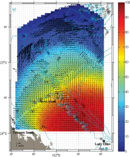
current data from ADCP moorings located around Heron Island (Fig.1).

Figure 1. Map of the area of study showing the location of the two radar stations (Tannum Sands and Lady Elliot Island) and of the three ADCP mooring stations (small squares; see detail in Fig. 5), and a snapshot of surface current vectors (26/10/07 at 9:40 am; local time) produced by the

HRF and the percentage of valid (non-NaN) observations for the period between 16/10 and 16/11/2007 on each grid point (4 km spacing).

II. METHODS

A. Computation of the HFR currents from radials

A pair of HFR (WERA, Helzel Messtechnik GmbH) were deployed at Tannum Sands and Lady Elliott Island, to provide remotely sensed surface currents on an equispaced grid at intervals of 4 km, with an overlapping coverage area centred on Heron Island (23.5ºS, 152ºE; Fig. 1). The radar operating range is often beyond 150 km. Each single station produces a

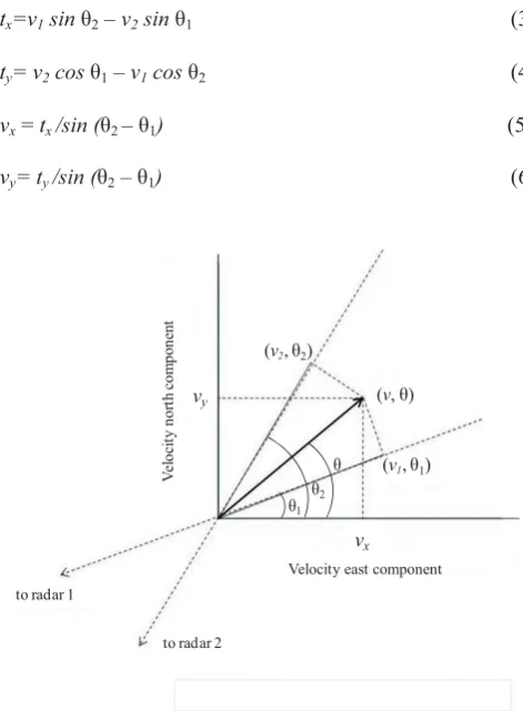
component of the surface current velocity directed toward or away from the radar, called radial velocity component. Therefore, the 2D surface current velocity vector magnitude and direction (v, ) can be extracted by adding the two radial velocity components (v1, 1) and (v2, 2) obtained at each

radar station (Fig. 2) as follows:

v2=vx2+vy2 (1)

=tan-1(ty/tx), (2)

where vx and vy correspond to the components of surface current vector with velocity (v) along the x and y axis, and tx and ty are parameters given by: tx=v1 sin 2 – v2 sin 1 (3)

ty= v2 cos 1 – v1 cos 2 (4)

vx = tx /sin (2 – 1) (5)

vy= ty /sin (2 – 1) (6)

Figure 2. Schematic diagram of the two radial velocity components (v1, 1) and (v2, 2) and the resultant surface current velocity vector magnitude and direction (v, ). The origin is the scattering point on the sea. B. Data and tidal analysis The data used in this study encompassed the period between 16/10/2007 and 16/11/2007, when the radar stations became operational. The Acoustic Doppler Current Profiler (RDI Workhorse ADCP) data for the same period were obtained from three moorings located north (H1), east (H2) and south (H3) of Heron Island (Fig.1). The ADCP current velocity through the water column was recorded every 30 minutes. The HFR and ADCP data are available at http://www.imos.org.au/. The HFR data obtained every 10 minutes were temporally averaged over 30 minutes. The data used were ‘first-look’ non-quality controlled, and as a precaution against noise spikes, velocities above 1.5 m s-1 were discarded. When these data are re-processed for the permanent archive there will be an improvement in the data quality. The root mean square difference (rms) was calculated as follows: rms=((di–)2/N), (7)

where di is the individual difference between the HRF and ADCP absolute current velocities, is the average of all individual differences, N is the total number of observations and i=1, 2...N. Time series of Eulerian current velocity measured at H1, H2 and H3 moorings at a depth of about 5.5 m were used to compute the progressive vectors assuming that the current values were uniform over the focused area. The ADCP data measured at 22 to 36 different depths (bins) were used to perform the tidal analysis for the period between 16/10/2007 and 16/11/2007. The t_tide package was used [10], removing any constituent with a period greater than 33 h. The same procedure was adopted to perform the tidal analysis of the HFR surface current data extracted for the same geographic coordinates of the moorings at these three locations. The HFR current velocity data were present for 55% (H1), 75% (H2) and 63% (H3) of the analysed month. C. Simulation of the Lagrangian tracking The Lagrangian advective paths were computed using the nonlinear differential equation describing the motion of a particle in a two-dimensional velocity field, as in dr(t)/dt=v(t), (7)

where r=(x,y) denotes the position of the particle on a UTM grid and v(t) is the Lagrangian velocity vector; both terms are time-dependent. This equation is solved using the Euler predictor-corrector method and Redfearn’s formulae [2] to project the tracking coordinates at each instant of time on a UTM grid. A bilinear interpolator was used to obtain velocity speed and direction from the HFR map at every new position and corresponding instant of time.

III. RESULTS

Comparison between ADCP and HFR data

A reasonable agreement was found between the HFR and the ADCP absolute current speeds during the analysed month, with the difference between them less than ± 0.15 m s-1 in 68% of the observations at the three mooring stations (Fig. 3). There is a bias in the histogram in Fig. 3 showing that radar currents on average are higher than ADCP currents. This is expected because of the wind effects at the surface. Larger differences were usually associated to a few spikes in the data. The rms for all data is 0.18 m s-1. This value is a bit high probably due to the presence of spikes in the radar data; however it is within the rms range (0.07–0.20 m s-1) observed in other studies [4, 12]. These are raw data; we expect spikes to be removed in quality control processing of the radar data. Further, linear regression between the HFR and ADCP u-component velocities (cross-shelf) produced significant r2

1

2

vy

vx Velocity east component

V el o ci ty n o rt h co m p o n en t

to radar 2 to radar 1

(v2, 2)

(v, )

between 0.5-0.7 for the three locations, although a poorer regression was observed for the v-component, as exemplified in Fig. 4.

Figure 3. Histogram showing the number of observations per class interval (m s-1_{) of the difference between the HFR and ADCP absolute current}

velocities for all data including the three moorings.

Discrepancies between these data sets can arise because the HFR data integrates the surface current averaged over a depth of 1.5 m and over a grid cell (4x4 km) while the shallowest valid ADCP data are sub-surface (depth of 5.5 m) single-point measurements. As the tidal signal was more accentuated on the cross-shelf velocity component (u), it is expected to show a better agreement between the HFR and ADCP at any depth.

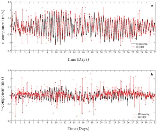
Figure 4 (a) Temporal variation of the u (east) and (b) v (north) current components at H1 mooring station (black) and the HFR data (red) superimposed for the period between 16/10/2007 and 16/11/2007.

On the other hand, the north-south current (v-component) presented a bigger influence of wind driven and shelf processes, which vary to a larger extent with depth (see Table I). This will be discussed next.

Tidal influence at the mooring stations

Tides explained 89-96% of the total current temporal variability considering all ADCP measurements (depths between 5.5-47.5 m) at H1 and H3 mooring stations, and between 42 and 79% at H2 station. In general, surface HFR currents were less influenced (60-69%) by tidal forcing than currents measured at about 5.5 m depth (moorings), during the analysed month. Further, the current speed variation explained in terms of tidal forces decreased from the bottom (40-47 m depth) to the surface (1.5 m depth), suggesting an increasing influence of the wind driven circulation close to the surface (see Table I).

The percent of variance explained by the tidal forcing was higher for the u-component (cross-shelf) than the v-component (north-south), especially at the surface (HFR data) (see Table I).

TABLE I

PERCENTOFVARIANCEPREDICTEDOVERTHEORIGINAL

VARIANCEFORTHETOTALTIDALANALYSIS,FORTHEUAND

V-COMPONENTESATDIFFERENTWATERDEPTHS(M)

depth total variance variance (u) variance (v)

H1_mooring 40.5 95 97 89

H1_mooring 5.5 89 91 81

H1_HFR 1.5 69 80 20

H2_mooring 47.3 74 90 51

H2_mooring 5.3 42 45 36

H2_HFR 1.5 60 73 25

H3_mooring 40.5 94 95 78

H3_mooring 5.5 89 93 46

H3_HFR 1.5 68 82 17

The north-south current velocity component is likely to be influenced by the strong south-easterly and northerly winds that prevail at Heron Island region in the months of October and November (Bureau of Meteorology of the Australian Government; http://www.bom.gov.au/climate/ averages/tables/ cw_039122.shtml).

Additionally, the stations located on the shelf north (H1) and south (H3) of Heron Island in the middle of channels between two reefs showed a clearer tidal signal than the station situated to the east of the island (H2) (Fig. 1). The H2 station is situated on the shelf break outside of the reefs, where a bigger influence of the East Australian Current (EAC), the wind-driven circulation and friction induced by topography, is expected. This is evidenced also in the velocity profiles where larger differences in the current speed and direction between the surface and bottom layers occurred at H2 (east) compared with H1 (north) and H3 (south).

Lagrangian trajectories

Fig. 5a shows the Lagrangian HFR paths and progressive vectors started at the H1, H2 and H3 stations. Separation distances between the HFR and ADCP based tracks can reach about 19-32 km after 2 days (Fig. 5b). These large differences occurred because the Lagrangian paths obtained from HFR data and the progressive vectors from ADCP measurements, started at H1 and H3 stations, went to opposite directions. As

u

-co

mp

o

n

en

t (

m

/s

)

Time (Days)

Time (Days)

v

-co

mp

o

n

en

t (m/

exemplified in Fig. 1, current vectors can point to the north in the proximity of H1 and H3 stations and then move south-east a few kilometres away. Tracks started at H2 headed in the south-east direction, but the HFR tracks reached deeper waters on the shelf break while the H2 progressive vector was confined between the 50 and 100 m isobath. The HRF tracks travelled longer distances than the progressive vectors. The tracks started exactly at H2 travelled about 47 km and 33 km in 2 days for the HFR and ADCP based paths, respectively. The separation distance between each one of four HFR tracks and the central track started at the stations was preserved during the 2 days tracking, varying usually less than ±2 km (maximum of 4 km).

These simulations have shown that the Lagrangian trajectories are sensitive to the starting location, and that the spatial variability of the currents has to be taken into account when tracking particles in time. During the analysed month, the radar tracking was usually aborted after a few hours or days because trajectories reached a region with no information on the current field. It is common to have areas of missing HFR data in the afternoon and evening due to ionospheric and/or radio-wave interference. Fig. 1 shows the number of valid observations (non-NaN) during the analysed month at each HRF grid point. The best temporal and spatial coverage

is obtained close to the radar stations, and the signal deteriorates with increasing distance from the stations. The current vectors are more correct for the area south of 23°S. It is worthwhile to mention that Fig. 1 is only valid for the analysed month and much better or worst temporal and spatial coverage can be observed in different periods of time. One challenge in applying Lagrangian tracking to management and operational tasks is to deal with the gaps in HFR data which inevitably arise because of noise and interference in the radio frequency spectrum. This can be addressed by assimilating good data into models for the current flow [11], and then using the model to assist the interpolation.

The second challenge is to take account of the errors in Lagrangian tracking from HFR data. From this and other work the error is of the order of 0.07–0.20 ms-1. If the tracking is done by interpolating in the time and space dimensions using raw measured surface velocities then the full impact of the errors is experienced. If the tracking is done by fitting a model and then producing tracks from the model, then the model inherently smooths out small fluctuations (as well as errors) and the resulting tracks are not realistically reproducing the advection scales of the surface water; effectively the small scale processes are modelled by zero diffusivity. This is a critical area of ongoing research.

Figure 5 (a) Lagrangian paths from HFR currents (light red), progressive vector from ADCP currents (blue) starting at H1, H2 and H3 stations. The HFR data was used to plot another 4 tracks starting on the corners of 8 km squares centred at each one of the three stations (dark red lines). The starting point is indicated by an asterisk (*) and the tracking lasted 2 days or less, starting on the 26th _{of October 2007 at 9:40 am (local time). The stars show the locations}

of the two HFR stations located at Tannum Sands and Lady Elliot Island; and the grey squares show the location of the three mooring stations located around Heron Island: H1 (north), H2 (east) and H3 (south). Bathymetry contours (m) are shown in blue; (b)Separation distance (km) between the HFR and mooring tracking coordinates for the tracks starting at H1, H2 and H3 stations. The separation distance was calculated as the square root of the sum of

the squared difference between the HFR and mooring Easting and Northing coordinates.

(

a

)

0 5 10 15 20 25 30 35

0.0 0.5 1.0 1.5 2.0

H1 H2 H3

Time (Days)

se

pa

ra

ti

o

n (

K

m

)

IV. CONCLUSION

The HF-radar data allows inclusion of the spatial current variability in the track computation with a high temporal resolution. This is a significant improvement on the Eulerian approach because tracking depends on spatial inhomogeneity of the surface current field. This is particularly important for the study region where the currents exhibit a large spatial variation imposed by tides, winds, large scale circulation and topography. One issue with HFR tracking at the moment is the need to fill gaps in the data sets, both in space and time. This can be solved by applying and validating current estimation-interpolation techniques to fill the gaps, or by assimilating the data into a model which produces Lagrangian tracks. The biggest issue to be addressed is the verisimilitude of the tracking when small scale fluctuations in surface velocities are ignored.

ACKNOWLEDGMENT

This work forms part of the Integrated Marine Observing System within the National Collaborative Research Infrastructure Strategy in Australia and data were obtained from the Integrated Marine Observing System (www.imos.org.au). Data were provided by the Australian Government’s National Collaborative Research Infrastructure Strategy and the Super Science Initiative and funding was also through the Queensland Department of Tourism, Regional Development and Industry.

REFERENCES

[1] A.J. Abascal, S. Castanedo, R. Medina, I.J. Losada, E.A. Fanjul, Application of HF radar currents to oil spill modelling. Mar. Poll. Bull., vol. 58, pp. 238-248, 2009.

[2] A.H.Q. Survey Coy., 1942, A.H.Q. Survey Coy by Authority of Director of Survey, 1942.

[3] K.P. Edwards, J.A. Hare, F.E. Werner, B.O. Blanton, Lagrangian

circulation on the Southeast US Continetal Shelf: Implications for larval dispersion and retention. Cont. Shelf Res., vol. 26, pp. 1375-1394, 2006. [4] H. H. Essen, K. W. Gurgel, T. Schlick, On the accuracy of current

measurements by means of HF radar. IEEE J. Oc. Eng., vol. 25 (4), pp. 472-480, 2000

[5] S. Gaskin, L. Kemp, J. Nicell, Lagrangian tracking of specified flow parcels in an open channel embayment using phosphorescent particles, ASCE Conf. Proc. 113, 19, 2002.

[6] G. Gawarkiewicz, S. Monismith, J. Largier, Observing larval transport processes affecting population connectivity progress and challenges.

Oceanography, vol. 20 (3), pp.40-53, September 2007.

[7] H.C. Graber, B.K. Haus, L.K. Shay, R.D. Chapman, HF radar comparisons with moored estimates of current speed and direction: Expected differences and implications. J. Geophys. Res., vol. 102, pp.18,749-18,766, 1997.

[8] M. R. Larson, M. G. G. Foreman, C. D. Levings, M. R. Tarbotton, Dispersion of discharged ship ballast water in Vancouver Harbour, Juan De Fuca Strait, and offshore of the Washington Coast. J. Environ. Eng. Sci., vol. 2, pp.163–176, 2003.

[9] P.R. Oke, P. Sakov, E. Schulz, A comparison of shelf observation platforms for assimilation in an eddy-resolving ocean model, Dyn. Atmos. Ocean., vol. 48 (1-3), pp. 121-142, 2009.

[10] R. Pawlowicz, B. Beardsley, S. Steve Lentz, Classical tidal harmonic

analysis including error estimates in MATLAB using T TIDE. Comp.

Geo., vol. 28, pp. 929–937, 2002.

[11] D. S. Ullman, J. O’Donnell, J. Kohut, T. Fake, A. Allen, Trajectory prediction using HF radar surface currents: Monte Carlo simulations of prediction uncertainties. J. Geophys. Res., vol. 111, C12005, 2006. [12] Y. Yoshikawa, A. Masuda, K. Marubayashi, M. Ishibashi, A. Okuno, On