Advancing implementation conditions of optimal experimental design for dual response systems using one continuous response and one binary response

Rochester Institute of Technology

RIT Scholar Works

Theses

4-26-2019

Advancing implementation conditions of optimal

experimental design for dual response systems

using one continuous response and one binary

response

Rory W. Little

[email protected]

Follow this and additional works at:https://scholarworks.rit.edu/theses

This Thesis is brought to you for free and open access by RIT Scholar Works. It has been accepted for inclusion in Theses by an authorized administrator of RIT Scholar Works. For more information, please [email protected].

Recommended Citation

Advancing implementation conditions of optimal experimental design for

dual response systems using one continuous response and one binary response

Thesis Defense

Rory W. Little

Rochester Institute of Technology

Thesis Advisor: Dr. Rachel Silvestrini

Committee Member: Dr. Katie McConky

Approval Date: April 26th_{, 2019}

i DEPARTMENT OF INDUSTRIAL AND SYSTEMS ENGINEERING

KATE GLEASON COLLEGE OF ENGINEERING

ROCHESTER INSTITUTE OF TECHNOLOGY

ROCHESTER, NY

CERTIFICATE OF APPROVAL

M.S. DEGREE THESIS

The M.S. Degree thesis of Rory Little

Has been examined and approved by the

Thesis committee as satisfactory for the

Thesis requirements for the

Master of Science degree

Approved by:

Dr. Rachel Silvestrini Date

Thesis Advisor

Dr. Katie McConky Date

ii

Abstract

Optimal designs are computer-generated experimental designs that provide an

experimenter with an ‘optimal’ set of experimental trials. Historically, optimal experimental

design has been limited to optimization with regards to a single criterion for a single response

variable. Recent research by Burke et al. (2017) made it possible to create a dual response

optimal designs for cases involving experiments with one continuous response and one binary

response. The algorithm in Burke et al. (2017) provides a series of weighted optimal designs

across a range of weights between the continuous and binary response cases. This thesis extends

the work by Burke et al. (2017) in three ways. First, a new optimality criterion is developed in

order to provide more stable algorithm results. Second, a method for selecting the weighted

design that provides the best results for the continuous and binary cases is developed. Finally, a

sensitivity analysis on the prior information required to generate the optimal designs in

iii

Table of Contents

1 Introduction ... 1

2 Background and Literature Review ... 9

2.1 Optimal Designs for Multiple Criterion ... 9

2.2 Optimal Designs for Multiple Responses ...11

3 Burke’s Algorithm ... 16

3.1 Proposed Normalized Binary Criterion ... 16

3.2 Validation of Proposed Criterion ... 18

4 Methodology ... 23

4.1 Estimating 𝑊𝐶𝑂 using fitting techniques ... 26

4.2 Experiment to Vary Model Configurations ... 31

5 Results ... 35

5.1 Impact of Estimation Error on Design Relative Efficiencies ... 35

5.2 Impact of Model Configurations on Compromise Optimal Designs ... 38

5.2.1 Main Effects Model Configurations ... 42

5.2.2 Main Effects & Two-Factor Interaction Model Configurations ... 46

5.2.3 Main Effects, Two-Factor Interaction & Quadratic Model Configurations ... 49

6 Conclusions & Future Work ... 53

6.1 New Normalized Binary Criterion ... 53

6.2 Fitting Technique Estimation Method... 54

6.3 Sensitivity of Prior Model Configurations ... 55

6.3.1 Sensitivity of the Mean Parameters ... 55

6.3.2 Sensitivity of the Mean Parameter Uncertainties ... 56

6.3.3 Sensitivity of the Number of Trials ... 56

6.3.4 Conclusions & Future Work of Sensitivity Experiments ... 57

Works Cited... 59

Appendix A ... 61

1

1 Introduction

Experiments are fundamental for developing an understanding of the world around us.

They allow us to deduce the cause-effect relationships active in a given system. However, these

deductions are based on the assumption that an experiment is properly designed. Statistically

designed experiments provide an objective and organized method for investigating how a set of

control variables affect a response variable of interest (Montgomery, 2017).

An experimental design defines the series of experimental conditions, otherwise called

trials or runs. Each trial specifies the value of the control variables manipulated as part of this

experiment. Designed experiments range from simple to difficult, depending on the situation or

system in question. An experiment with many response variables is an example of a situation

where designing an appropriate experiment can be difficult. This is because different response

variables can benefit from very different experimental design approaches. If experimentation is

cheap, more trials could be run to improve results incrementally in lieu of an ideal design. When

experimentation is expensive, additional trials may not be possible. In this case, a method for

selecting an ideal design is necessary to keep experimentation costs within budget.

Consider a toy rocket experiment in which travel height and parachute deployment are

identified as important responses of interest. Height is a continuous variable (meters) and

parachute deployment is a binary variable (1 = deployed and 0 = did not deploy). The cost of

running each trial is relatively low and collecting the data would be trivial. However,

experimentation on real rockets is more resource intensive and only a limited number of trials

could be run. SpaceX exemplified this restriction, conducting single experimental trials

exceeding 90 million dollars (Goddard, 2018). In cases such as these, researchers must ensure

2 Experimental design methods are useful for making testing more economical. Results

with these approaches can be achieved with less investment of time or resources. One type of

experimental design is optimal experimental design. Optimal experimental design is a method

which maximizes the amount of information gained from the experiment when the number of

trials is constrained. The settings in the resulting design are chosen to maximize the probability

of improving the model of interest. Unlike traditional factorial designs, optimal experimental

designs require prior knowledge of the system being studied for generating the design. An

optimal approach can work well when prior system knowledge is available, but results suffer if

little is known about the system. Optimal design is further complicated with the addition of

multiple responses.

Practitioners represent their prior knowledge of a system as a model equation, referred to

as the prior response model in this research. The prior response model defines the expected

relationship between the control variables and the response. Control variables are also known as

factors, in experimental design. Consider the toy rocket example where two factors will be

manipulated, launch pressure (𝑥₁) and rocket body length (𝑥₂). One prior response model is

needed for each of the two responses.

The continuous response could be modeled using a linear model such as,

𝑦1𝑁 = 𝛽0+ 𝛽1𝑥1+ 𝛽2𝑥2+ 𝜀 (1)

where 𝑦_1𝑁 is the continuous response variable (launch height in meters) and 𝛽₀, 𝛽_1, and 𝛽₂ are

the model parameters. The binary response can be modeled using a logistic regression model

such as,

𝑦_1𝐵 = 1

3 where 𝑦1𝐵 is the binary response variable (parachute deployment) with model parameters 𝜃0, 𝜃1

and 𝜃₂. These prior response models are not only required, but also important in the generation

of optimal designs.

Optimal designs are computer-generated designs that are created to provide the ‘optimal’

set of trials (N) in an experimental design, given a set of constraints imposed by the practitioner. Typically, this is achieved with computer software which optimizes an objective function related

to the quality of the assumed form of the model (prior response model). The practitioner provides

the number of trials and the assumed model to relate the response (𝑦) to the factors (𝑥₁, … , 𝑥_𝑘)

manipulated during experimentation for example see the models shown in Equation 1 and 2. The

most common optimal designs are those with the letter-based naming convention, including: A -Optimal, D-Optimal, G-Optimal, and I-Optimal. Each of these designs are based on different criterion values that provide designs intended to meet different practitioner needs. These designs

are referred to as 'alphabetic optimal designs' because of the letter naming convention. As an

example, the D-Optimal design is one in which the set of trials, or runs, in an experiment are chosen to minimize variance of the regression coefficient estimates. For information on optimal

design see Montgomery (2017), Myers, Montgomery, and Anderson-Cook (2016), and Goos and

Jones (2011).

Optimal design for each response and associated prior response model can be generated

using computer software. The inputs required from the experimenter for the software will be

referred to as the model configuration in this research. A model configuration is defines the

response, input (controllable) variables, the prior response model, the optimality criterion, and

the number of trials. The design is then created and provided in the form of a table with each trial

4 useful tool for visualizing any experimental design, including optimal designs, utilizes a design

plot. An example of design plots are provided in Figure 1. Each point in the design plot

represents an experimental trial at corresponding levels of each of the factors (normalized

between −1 and 1). The design space is the area representing any potential experimental trial.

Both experiments shown in Figure 1 are limited to eight trials each and the ‘2’ in Figure 1a

indicates two trials of equivalent input settings.

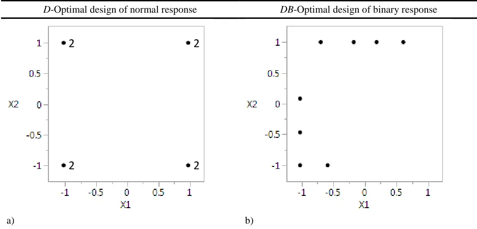
D-Optimal design of normal response DB-Optimal design of binary response

a) b)

Figure 1: Comparison of optimal designs for a normal response versus a binary response

Figure 1a is the D-Optimal design for a normal response variable with the assumed model form of Equation 1. Logistic regression requires the use of a Bayesian statistical process to make

the design seen in Figure 1b. It is referred to as the Bayesian D-Optimal (DB-Optimal) design.

DB-Optimal design, like the D-Optimal design, uses an objective function related to the quality of the regression coefficients. However, it requires an information matrix with a link function

related to the logistic response to be created. Non-linear optimal experimental designs, such as

the logistic case, rely on the model and the distribution of the parameters contained in it to

generate a design. Misspecification of the model parameters and their associated uncertainties in

2 2

5 relation to their values can result in sub-optimal designs as discussed in Johnson & Montgomery

(2009).By contrast, the D-Optimal design is does not rely on the distribution of the parameters contained in the model.

Note that the points of Figure 1a and 1b appear at very different locations in the plot.

Comparing design plots visually can provide a good sense of how similar the designs are. The D -Optimal design for the normal response generates trials in the extreme corners of the design

region (Figure 1a). While the D-Optimal design shows that the binary response variable favors trials along the left and top boundaries of the region (Figure 1b). Figure 1 shows that different

types of responses, such as the continuous and binary response, generate very different optimal

designs. This presents a challenge when developing a single optimal design for both responses

together.

The relationship between the DB-Optimal design and its prior response model can be visualized by overlaying the design plot and the probability contour plot of the binary response

in the design space. The contours are generated by the response expectations as defined by the

prior response model. Figure 2 illustrates the relationship between experimental trials from

6

Figure 2: Design Contour Plot of DB-Optimal design

This single optimal design will possess a blend of experimental trials which are desirable

for both responses. There are several ways to evaluate the quality of an experimental design. One

way is to calculate a metric called the design efficiency. A design efficiency captures how well a

particular design will work in comparison to an ideal design or another design of interest. Design

efficiency metrics, which range from 0 to 100, can be used to compare designs, where higher

efficiencies indicate better performance. Two efficiency metrics are of interest, the D-Efficiency

(𝐷_𝑒𝑁_{) and DB-Efficiency (𝐷}

𝑒𝐵). These efficiency metrics are used to represent the extent in which

the design minimizes the error of the parameter prediction (𝛽𝑛or 𝜃𝑛). 𝐷𝑒𝑁 is the efficiency of a

particular design in relation to the D-Optimal design. 𝐷_𝑒𝐵 _{is similar but instead is compared to the}

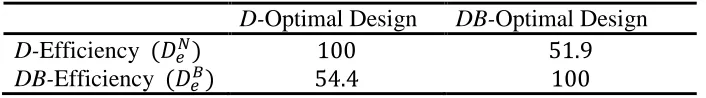
DB-Optimal design. The efficiencies for the example designs from Figure 1 are calculated and summarized in Table 1. A desirable design for both responses would be one in which the single

design performed well in both criteria. Table 1 indicates that neither design works well for both.

Table 1: Design efficiencies for normal and binary response

D-Optimal Design DB-Optimal Design

D-Efficiency (𝐷_𝑒𝑁) 100 51.9

7 Similar to the conclusion made from the visual comparison, these designs are also rather

different when comparing design efficiency. If only one design could be run, the experimenter

would need to determine which response was more important to accurately model. A better

design selection if both responses were of equal importance would have comparable efficiencies

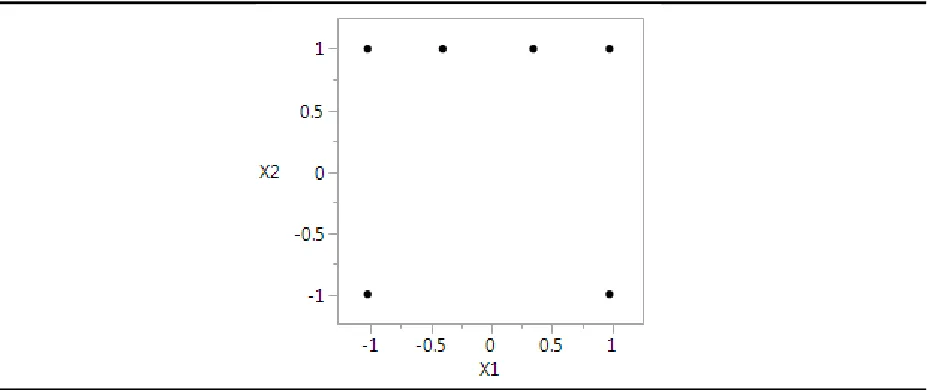
for each response. A slightly better suited design for this experiment is illustrated in Figure 3.

This experimental design produces 𝐷_𝑒𝑁 = 92.5 and 𝐷_𝑒𝐵= 71.8, indicating that this design is a

better middle ground for each response. This design also appears to share properties from both

D-Optimal and DB-Optimal designs. There are trials in the corners as seen in the D-Optimal design in Figure 1a and some points along the top edge of the plot similar to the DB-Optimal design in Figure 1b.

Figure 3: ‘Compromise’ Experimental Design

Creating an ideal design for these two responses requires some new methods to balance

the design requirements for each response. Burke et al. (2017) developed a weighted D-Optimal and DB-Optimal design for the case in which two responses, one continuous and one binary, will be collected (𝑦_𝑁, 𝑦_𝐵). The Burke et al. (2017) algorithm does not output a single design, but

instead a set of possible designs. A set of designs is desirable when one response may be more

8 needs. In the case where both responses are equally important, the ideal design possesses 𝐷_𝑒𝑁=

𝐷_𝑒𝐵 _{and both efficiencies are as large as possible. This research will refer to this special case}

design as the compromise optimal design. Figure 3 presented a design which is closer to a

compromise optimal design than the designs shown in Figure 1 but not quite balanced enough.

There is an opportunity to use the Burke et al. (2017) algorithm to find the compromise optimal

designs paired with some new approaches presented in this research.

There are two main objectives in this thesis research. The first objective is to provide a

methodology a practitioner may follow to find the compromise optimal designwhen considering

a dual response optimal experimental with a continuous and binary response variable of equal

importance. This methodology will be a supplementary tool to the dual response optimal design

algorithm developed by Burke et al. (2017). The second objective is to explore the sensitivity of

the model configurations, specifically the prior response model and the number of trials, on the

generation of compromise optimal designs. A third objective was completed to fulfill the

original two objectives. This objective was propose a new optimality criterion for Burke’s

algorithm to allow proper generation of dual response optimal designs for all model

configurations tested in this research.

In Section 2, a review of the literature is presented. Section 3 introduces a modification to

the criterion used in Burke’s algorithm. Section 4 outlines the methodology used to conduct this

research. Section 5 reviews the results and analysis completed for this research. Section 6

9

2 Background and Literature Review

The literature in this section covers background research concerning the creation of

optimal experimental designs for multi-response systems. Specifically, we explore how single

response optimal design helped inspire a dual response method. Extensions to the single criterion

optimal design include the cases of 1; optimal design for multiple criterion and 2; optimal design

for a single criterion, but multiple responses.

2.1 Optimal Designs for Multiple Criterion

In the Introduction (Section 1) we discussed that different optimal designs are created to

meet varying needs by using a specific type of alphabetic optimal design and specific design

criterions. The criterion result in the development of the optimal design with different properties.

These optimal designs require the use of search algorithms which maximize or minimize the

specified criterion. However many applications require solutions that meet multiple needs and

therefore require the use of multiple criterions. The most popular solution for doing this in the

design of experiment’s domain is combining the multiple criterions into a single function

referred to as a desirability function. This new function then works the same as if it were just a

single criterion. Desirability functions were proposed by Harrington (1965) and later expanded

by Derringer and Surich (1980). The desirability method combines multiple criterions into a

single objective function, controlling the relative impact of each criterion with weights. The

weights for all criteria sum to 1. Thus far, no more than two criterions have been combined using

a desirability function for optimal experimental design.

The selection of the appropriate combination of weights to use can be difficult because

they are primarily based on the practitioner’s judgment and they change from case to case. A

10 possibility that if the assumed weight pair (for the two criterions) is incorrectly tuned, the

resulting design can be sub-optimal (Derringer and Surich, 1980). The choice of weight given to

each criterion can have a large impact on the results and are quite sensitive in practice (Lu et al.

2011). To mitigate this risk, Lu et al. (2011) and Lu et al. (2014) created a set of experimental

designs using many possible weight alternatives. Lu et al. (2011) proposes the use of a

desirability function coupled with a pareto frontier search algorithm to make the weight selection

process more transparent to the experimenter. The set of alternate experimental designs are

compared using tradeoff plots of performance metrics for each associated performance criterion.

Since initial fixed weight combinations are seen as subjective, Lu et al. (2011) recommends a

method which incorporates these weights into the algorithmic method and provides choices for

the experimenter.

A recent example of optimal designs with multiple criteria is Pan & Yang (2014). They

improved accelerated life testing plans by creating designs which balanced the D-efficiency criterion and I-efficiency criterion using a desirability function. They incorporated an efficiency tradeoff plot which was used to visualize the levels of D-efficiency and I-efficiency at different weight values. This process improved the conventional method by providing transparency to the

both efficiencies simultaneously, rather than just one. They showed how this desirability

approach was a significant improvement over the optimum split design method used in this field

previously.

Similarly, Lu et al. (2014) created a method which combines D-efficiency and 𝑡𝑟(𝐴𝐴′)

performance metrics in a single optimizing function. They further improve computational time of

11 specified expectations. Although these methods handle many optimizing criteria, they still only

consider a single response.

2.2 Optimal Designs for Multiple Responses

Optimal design for multiple responses builds on the research described in Section 2.1.

Burke et al. (2017) created a weighted D-Optimal and DB-Optimal design approach for the multiple response experimental design problem. Here, two responses with different prior

response models are considered. First, a continuous response using an assumed standard linear

regression prior response model and second, a binary response variable using an assumed logistic

regression prior response model. Burke et al. (2017) proposed a desirability function which

combined the D-Optimal criterion for the continuous response and the Bayesian D-Optimal criterion for the binary response into a single objective function. Their research has made it

possible to compare these tradeoffs properly using a weighted desirability function.

The approach proposed by Burke et al. (2017) differs from the pareto frontier method

used in Lu et al. (2014). Instead, they created an optimal design at many different weight

combinations between 0 and 1. Then, Burke’s algorithm loops through these weight

combinations, generating an optimal design for each. Each optimal design is generated using a

coordinate and row exchange algorithm. This algorithm iteratively makes better and better

experimental designs through changing specific trials and factor levels until the objective

function (desirability function) can no longer improve.

The coordinate and row exchange algorithm proposed in Burke et al. (2017) was

designed for two responses from two model forms. To accomplish this, they incorporated search

12 desirability criterion was used to create the set of optimal designs for consideration of the

practitioner.

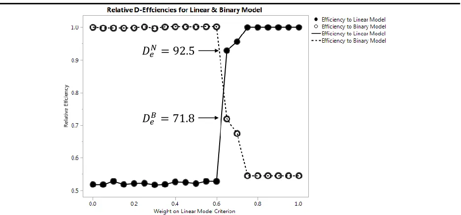
One method for comparing the designs proposed in Burke et al. (2017) is through the

relative efficiency plot. Figure 4 shows a relative efficiency plot for weighted optimal designs

with one continuous linear regression model assuming the structure of Equation 1 and one binary

response assuming a logistic regression model structure seen in Equation 2. The weight of the

D-Optimal criterion (𝑊_𝑁) and DB-Optimal criterion (𝑊_𝐵) can be expressed as a pair, [𝑊_𝑁, 𝑊_𝐵] (such that 𝑊_𝑁+ 𝑊_𝐵= 1 and 𝑊_𝑁, 𝑊_𝐵 ∈ [0,1]). As convention, the relative efficiency plot uses

𝑊𝑁 as the horizontal axis. This research will simply use 𝑊𝑁 to refer to a weight pair since 𝑊𝐵=

1 − 𝑊𝑁. Designs for weight pairs in increments of 0.05 are created within this region, which

totals 21 generated optimal designs. The 𝐷_𝑒𝑁 _{and 𝐷}

𝑒𝐵 are calculated for each optimal design and

are plotted as a function of 𝑊𝑁. Relative efficiency plots illustrate how different weights result

in 𝐷_𝑒𝑁and 𝐷_𝑒𝐵 tradeoffs.

Figure 4: Relative Efficiency Plot from Burke et al. (2017)

Recall the design shown in Figure 3. This design corresponds to the optimal design

generated at 𝑊_𝑁= 0.65 in Figure 4, this design is shown with two efficiency values, 71.8 for the

𝐷_𝑒𝑁_{= 92.5}

13 binary case and 92.5 for the linear case. The methodology introduced in Burke et al. (2017)

provides designs using an array of weights, but Figure 4 doesn’t provide the 𝑊_𝑁 a practitioner

should choose when 𝑦_𝑁 and 𝑦_𝐵 are of equal importance. In this research, we define the weight

where 𝐷𝑒𝑁 = 𝐷𝑒𝐵 as the weight of the compromise optimal design and will be referred to as the

compromise optimal weight (𝑊_𝐶𝑂). Figure 4 shows an example where the 𝑊_𝐶𝑂 does not

necessarily exist in the subset of sampled 𝑊_𝑁, although it would be considered the best option if

more iterations were not conducted. Therefore the 𝑊_𝐶𝑂requires further attention to provide a

robust recommendation of the optimal design settings for this special case dual response optimal

design.

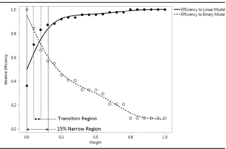
Figure 5 shows another example of the relative efficiency plot generated by Burke et al.

(2017) illustrating efficiency tradeoffs at different weights. In search of a 𝑊𝐶𝑂, we may reason

the 𝑊_𝐶𝑂would appear between weights where 𝐷_𝑒𝑁 _{> 𝐷}

𝑒𝐵 and 𝐷𝑒𝑁 < 𝐷𝑒𝐵. In this research, this

region of the relative efficiency plot will be referred to as the transition region. In this example, a

transition region appears between weight of 𝑊_𝑁 = 0.40 and 𝑊_𝑁 = 0.45, which indicates a

region where a compromise optimal solution is likely. The transition region in Figure 5 is labeled

14

Figure 5: Relative Efficiency Plot from Burke et al. (2017) (Main Effects & 2-Factor Interaction)

First, Burke et al. (2017) made it possible to generate dual response experimental designs

for the normal and binary responses, however there are some aspects of this method that remain

uninvestigated. While the relative efficiency plot does a good job of visualizing tradeoffs, but

there is no current method to find the precise 𝑊𝐶𝑂 to generate the compromise optimal design.

This thesis provides a practical approach using regression techniques to identify the compromise

optimal weight, 𝑊_𝐶𝑂, based on the results of the coordinate exchange algorithm developed in

Burke et al. (2017).

Second, Burke et al. (2017) found that misspecified parameters did have worse

performance than models with true parameter value and uncertainties. However, Burke et al.

(2017) did not capture the effect of each of the prior response model components and or the

number of trials. This thesis provides a sensitivity experiment to identify these effects.

While not originally one of the two thesis objectives, another research investigation was

required to complete the original objectives. We encountered some issues with the calculation of

the criterion used in the objective function of Burke’s algorithm. In Section 3, we discuss the Transition

15 issues that arose and the proposed solution used to ensure completion of the original two thesis

16

3 Burke’s Algorithm

A new optimality criterion is proposed to allow for generation of all model configurations

planned for this research. First, the proposed criterion is presented. Second, a validation of the

proposed criterion is discussed.

3.1 Proposed Normalized Binary Criterion

The normalized criterion for the binary response in Burke et al. (2017) was initially

constructed under the assumption that all criterions generated by Gotwalt’s algorithm were

negative. However, this assumption was not strictly upheld and as a result, violations of this

assumption resulted in the algorithm prematurely erroring. When the criterion is negative, an

imaginary number is generated when taking the square root the criterion value and causing the

algorithm to crash. Thus, an additional thesis research was conducted in order to create a new

normalized criterion for the binary response. This new criterion uses an alternative method for

normalization which requires a worst case value. The previous normalized binary criterion (𝜑̃𝐵)

proposed by Burke et al. (2017) was calculated using

𝜑̃𝐵_𝑂𝑟𝑖𝑔𝑖𝑛𝑎𝑙 =

𝜑_{𝐷𝐵−𝑂𝑝𝑡} 𝜑𝐵

(3)

The binary criterion for the DB-Optimal case (𝜑_{𝐵𝑖𝑛𝑎𝑟𝑦 𝐷−𝑂𝑝𝑡}) was calculated and divided by binary criterion of the design of interest (𝜑_𝐵). To complete this thesis research, Equation 3 was

replaced with

𝜑̃_{𝐵_𝑁𝑒𝑤} = 𝜑𝐵− 𝜑𝐵_𝑊𝑜𝑟𝑠𝑡𝐶𝑎𝑠𝑒 𝜑_{𝐷𝐵−𝑂𝑝𝑡}− 𝜑_{𝐵_𝑊𝑜𝑟𝑠𝑡𝐶𝑎𝑠𝑒}

(4)

For Equation 4 to work, a worst case binary criterion (𝜑_{𝐵_𝑊𝑜𝑟𝑠𝑡𝐶𝑎𝑠𝑒}) must be defined.

The criterion proposed in Equation 4, is shown to produce designs nearly identical to

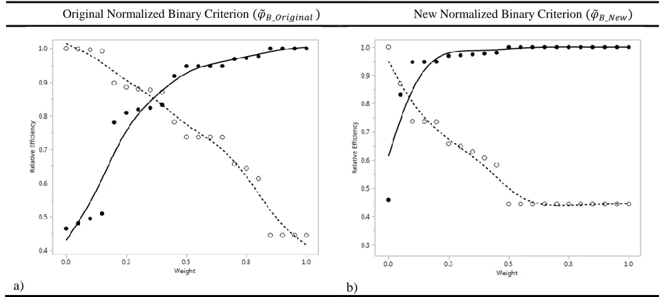
17 efficiency plot is shifted dramatically. Relative efficiency plots using 𝜑̃_{𝐵_𝑂𝑟𝑖𝑔𝑖𝑛𝑎𝑙} in Equation 3

tend to contain the 𝑊𝐶𝑂 between 0.1 and 0.7. When using 𝜑̃𝐵_𝑁𝑒𝑤in Equation 4, this is not the

case. Theoretically, 𝜑̃_{𝐵_𝑁𝑒𝑤} is expected to change the appearance of the relative efficiency plots,

but the extent to which the 𝑊_𝐶𝑂values changed is dramatic. Results showed the new criterion

shifts all of the observed 𝑊_𝐶𝑂 very close to 𝑊_𝑁= 0, with no 𝑊_𝐶𝑂 results exceeding 0.10. Figure

6 shows a transformation of relative efficiency plots from the original criterion (𝜑̃𝐵_𝑂𝑟𝑖𝑔𝑖𝑛𝑎𝑙 ) to

the new criterion (𝜑̃_{𝐵_𝑁𝑒𝑤} ) for a model configuration with a main effects and two-factor

interaction prior response model structure and 12 trials.

Original Normalized Binary Criterion (𝜑̃𝐵_𝑂𝑟𝑖𝑔𝑖𝑛𝑎𝑙 ) New Normalized Binary Criterion (𝜑̃𝐵_𝑁𝑒𝑤)

a) b)

Figure 6: Comparison of relative efficiency plots of a) (𝝋̃𝑩_𝑶𝒓𝒊𝒈𝒊𝒏𝒂𝒍 ) to b) (𝝋̃𝑩_𝑵𝒆𝒘 )

When using Equation 4, a practitioner may simply start the search for a compromise

optimal design at a narrower range, such as weights 0 to 0.15 in order to focus on primary

location of 𝑊_𝐶𝑂.

The new criterion provides a stable algorithm, but requires specification of the

𝜑_{𝐵_𝑊𝑜𝑟𝑠𝑡𝐶𝑎𝑠𝑒}, which is not a fixed number. The worst case continuous criterion value has a lower

18 worst case binary criterion is variable and may exist as positive or negative. Additionally, there

is no research regarding a proper way to calculate the 𝜑𝐵_𝑊𝑜𝑟𝑠𝑡𝐶𝑎𝑠𝑒. In an attempt to derive the

value empirically, extreme designs were created for a variety of model configurations to discover

the 𝜑_{𝐵_𝑊𝑜𝑟𝑠𝑡𝐶𝑎𝑠𝑒}.

This investigation yielded some key limits on the value of the worst case binary criterion

(𝜑_{𝐵_𝑊𝑜𝑟𝑠𝑡𝐶𝑎𝑠𝑒}). The range of lower limits across different model configurations was roughly -30

to -50. A lower limit of 𝜑_{𝐵_𝑊𝑜𝑟𝑠𝑡𝐶𝑎𝑠𝑒} = −50 prevents the algorithm from crashing for all

model configurations. There also appears to be a direct relationship between the 𝜑𝐵𝑖𝑛𝑎𝑟𝑦 𝐷−𝑂𝑝𝑡

and 𝜑_{𝐵_𝑊𝑜𝑟𝑠𝑡𝐶𝑎𝑠𝑒}. As the 𝜑_{𝐵𝑖𝑛𝑎𝑟𝑦 𝐷−𝑂𝑝𝑡} increased or decreased, 𝜑_{𝐷𝐵−𝑂𝑝𝑡} also did. This

relationship allowed the range of 𝜑_𝐵 to remain more stable across all cases. The range of

𝜑𝐷𝐵−𝑂𝑝𝑡 was approximately 2 to −12 and lowest lower limit was −50. Thus 𝜑𝐵_𝑊𝑜𝑟𝑠𝑡𝐶𝑎𝑠𝑒 for

each trial was calculated

𝜑_{𝐵_𝑊𝑜𝑟𝑠𝑡𝐶𝑎𝑠𝑒} = −40 + 𝜑_{𝐵𝑖𝑛𝑎𝑟𝑦 𝐷−𝑂𝑝𝑡} (5)

Using Equation 5, the model configurations which required a 𝜑𝐵_𝑊𝑜𝑟𝑠𝑡𝐶𝑎𝑠𝑒 ≅ −50 are accounted

for since they also had 𝜑_{𝐵𝑖𝑛𝑎𝑟𝑦 𝐷−𝑂𝑝𝑡}≅ −12. The model configurations with smaller

𝜑_{𝐵𝑖𝑛𝑎𝑟𝑦 𝐷−𝑂𝑝𝑡} didn’t require such a large 𝜑_{𝐵_𝑊𝑜𝑟𝑠𝑡𝐶𝑎𝑠𝑒}, so these cases are also accounted for,

meaning we do not anticipate the algorithm crashing.

3.2 Validation of Proposed Criterion

In order to validate the new normalized binary criterion and the associated relative

efficiency plots, the resulting compromise optimal designs were compared to ensure similar

results. Then, the optimal designs are compared and discussed. Finally, the narrow relative

19 Three optimal design examples from Burke et al. (2017) are used for validation of

𝜑̃𝐵_𝑁𝑒𝑤. Each of these examples required a series of steps to identify the compromise optimal

design. First, the original normalized binary criterion (𝜑̃𝐵_𝑂𝑟𝑖𝑔𝑖𝑛𝑎𝑙) was used in Burke’s

algorithm to generate a relative efficiency plot. Second, the transition region of this plot is

identified. Third, the algorithm was run again but instead with a narrower weight search region

surrounding the identified transition region to improve the ability to identify the 𝑊𝐶𝑂. This

resulting relative efficiency plot is referred to as the narrow relative efficiency plot in this

research. From the narrow relative efficiency plot, the 𝑊_𝑁 with the smallest difference between

𝐷𝑒𝑁 and 𝐷𝑒𝐵 was identified as the 𝑊𝐶𝑂. This 𝑊𝐶𝑂 corresponded to compromise optimal design of

interest. This process was repeated for the new normalized binary criterion(𝜑̃_{𝐵_𝑁𝑒𝑤}) and for

each of the three examples. A total of 3 pairs of compromise optimal designs were identified for

20

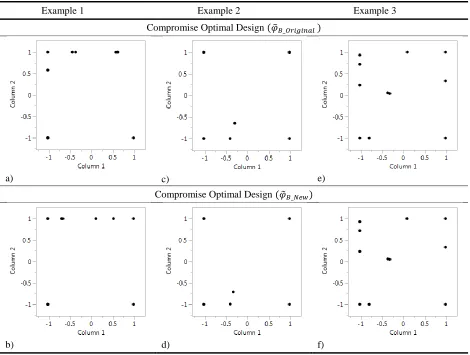
Example 1 Example 2 Example 3

Compromise Optimal Design (𝜑̃𝐵_𝑂𝑟𝑖𝑔𝑖𝑛𝑎𝑙 )

a) c) e)

Compromise Optimal Design (𝜑̃𝐵_𝑁𝑒𝑤)

b) d) f)

Figure 7: Comparison of compromise optimal designs

Example 1 in Figure 7 (a and b) show very similar, yet not exact, designs. Examples 2 (c

and d) and 3 (e and f) in Figure 7 show nearly identical compromise optimal designs. Since the

method for finding these designs is a discrete sampling method over a space, there are occasions

when the best 𝑊_𝑁 observed is not really the idealistic 𝑊_𝐶𝑂(𝐷_𝑒𝑁 = 𝐷_𝑒𝐵) but instead is the closest

𝑊_𝑁that was able to be sampled (𝐷_𝑒𝑁_{≅ 𝐷}

𝑒𝐵). The difference between 𝐷𝑒𝑁 and 𝐷𝑒𝐵 should be

minimized. More details regarding 𝑊_𝐶𝑂, 𝐷_𝑒𝑁and 𝐷_𝑒𝐵 are described in Section 4. The inability to

identify the idealistic 𝑊_𝐶𝑂 is best observed on the narrow relative efficiency plot. The narrow

relative efficiency plots for Figure 7 Example 1 are provided in Figure 8. These plots were used

to identify the 𝑊_𝐶𝑂 and therefore the compromise optimal designs for 𝜑̃_{𝐵_𝑂𝑟𝑖𝑔𝑖𝑛𝑎𝑙} (Figure 7a)

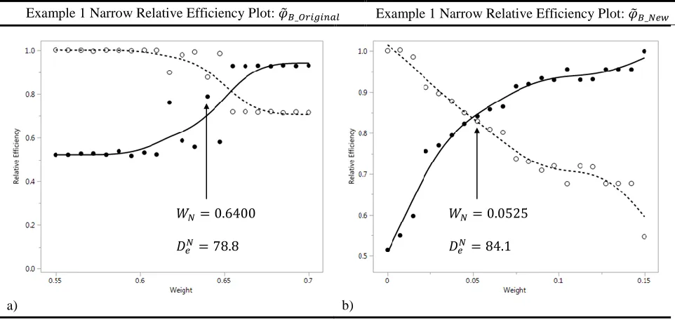
21 Example 1 Narrow Relative Efficiency Plot: 𝜑̃𝐵_𝑂𝑟𝑖𝑔𝑖𝑛𝑎𝑙 Example 1 Narrow Relative Efficiency Plot: 𝜑̃𝐵_𝑁𝑒𝑤

a) b)

Figure 8: Comparison of Example 1 Narrow Relative Efficiency Plots

While the difference in 𝑊𝐶𝑂 values among the new and original criterion is quite large for

for Example 1, the efficiency values at 𝑊_𝐶𝑂are not much different. The original criterion (Figure

8a) shows that the closest 𝑊_𝑁 to 𝐷_𝑒𝑁 _{≅ 𝐷}

𝑒𝐵 was 𝑊𝐶𝑂 = 0.6400, with a difference between 𝐷𝑒𝑁

and 𝐷_𝑒𝐵 of about 0.10. As discussed earlier, the idealistic 𝑊_𝐶𝑂 should create a design which has

𝐷_𝑒𝑁 _{= 𝐷}

𝑒𝐵. Contrary, the new criterion seen in Figure 8b provides a 𝑊𝐶𝑂 = 0.0525 and

corresponding design where the difference between 𝐷𝑒𝑁 and 𝐷𝑒𝐵 is only 0.01. The result provided

by the new criterion is better, based on the smaller difference between 𝐷_𝑒𝑁 _{and 𝐷}

𝑒𝐵. This

validation process did not originally suspect a difference in criterion performance but this result

suggests there could be.

Note that Examples 2 and 3 had narrow relative efficiency plots which had a more

gradual transition, similar to the one seen in Figure 8b. This allowed for the identification of a

𝑊_𝐶𝑂 with very small difference between 𝐷_𝑒𝑁 _{and 𝐷}

𝑒𝐵, thus making designs which were nearly

identical. An in depth analysis of these differences is presented later in Section 5.4. This shows

that the new proposed criterion produces nearly identical compromise optimal designs to the

𝑊𝑁= 0.6400

𝐷𝑒𝑁 = 78.8

𝐷𝑒𝐵 = 87.7

𝑊𝑁= 0.0525

𝐷𝑒𝑁= 84.1

22 original criterion. Additionally, the new criterion may provide smoother design efficiency

transitions in the relative efficiency plots based on the observations from Figure 8. This research

23

4 Methodology

In this section, the methodology used to study the two primary objectives of this research

is presented. First, a regression technique for detecting the compromise optimal weight 𝑊𝐶𝑂 is

discussed. Second, a sensitivity analysis of the model configurations is developed to study their

impact on the resulting optimal designs. The general procedure of this thesis methodology is

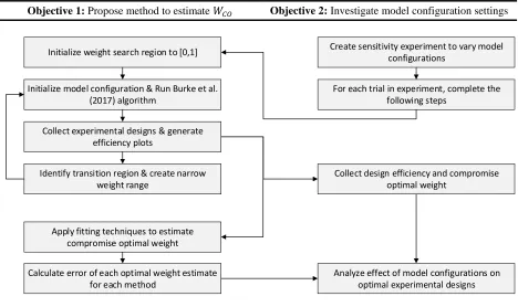
presented in Figure 9.

Objective 1: Propose method to estimate 𝑊𝐶𝑂 Objective 2: Investigate model configuration settings

Figure 9: Flow chart of experimentation process

This methodology is most clearly understood by first understanding how Burke’s

algorithm was used to generate the compromise optimal designs. This follows the first three

process boxes of Objective 1 in of Figure 9. However, first a brief summary of setting up Burke’s

algorithm is provided.

Burke’s algorithm was written in JMP scripting language (JSL) within the JMP Pro

software. The script can be compiled within this software to generate a dual response optimal

Collect experimental designs & generate efficiency plots

Identify transition region & create narrow weight range

Apply fitting techniques to estimate compromise optimal weight

Initialize model configuration & Run Burke et al. (2017) algorithm

Initialize weight search region to [0,1] Create sensitivity experiment to vary model

configurations

For each trial in experiment, complete the following steps

Collect design efficiency and compromise optimal weight

Calculate error of each optimal weight estimate for each method

24 design. The model configuration inputs that are being investigated in this research are the prior

response model structure, prior mean parameter value (𝛽_𝑛 or 𝜃_𝑛), prior standard deviation of the

mean parameter value (𝜎𝜃𝑛), and the number of trials available to the optimal design. Section

4.2 will further expand the different model configurations tested and refers to Objective 2 in

Figure 9.

When considering a single model configuration, the steps to identify a compromise

optimal design are as follows. The inputs specified by the model configuration (prior response

model, number of trials…etc.) are entered into the script. The code is run the first time to

calculate the DB-Optimal design, (𝑊_𝑁 = 0) to obtain the DB-Optimal design and DB-Optimal design criterion 𝜑_{𝐷𝐵−𝑂𝑝𝑡}. There is no search region, it completes only a single iteration at that

one 𝑊𝑁. The 𝜑𝐷𝐵−𝑂𝑝𝑡 is then used to calculate the 𝜑𝐵_𝑊𝑜𝑟𝑠𝑡𝐶𝑎𝑠𝑒 using Equation 5 and both

parameters are entered into the algorithm as constants.

The second time the algorithm is run the 𝑊_𝑁 search region is set to [0 : 1] with 𝑊_𝑁

increments of 0.05 (a total of 21 iterations). All else remains the same. When complete, the

algorithm outputs the 21 optimal designs to a comma separated value (.csv) file. This data file is

then used as input for a separate relative efficiency calculator created by Burke et al. (2017) to

generate the relative efficiency plots. The output of this is a JMP data table and a corresponding

relative efficiency plot (for example see Figures 4, 5 or 6).

The data provided in the relative efficiency plots is used to estimate the compromise

optimal weight (𝑊𝐶𝑂). As a note, this is where the process for the practitioner would stop. They

would inspect the relative efficiency plot to select a 𝑊_𝑁 and corresponding optimal design that

best fits their needs. However, our first objective of this research is to develop method for

25 again at a narrower region to find the true 𝑊𝐶𝑂. This can be used for accuracy comparisons for

the methods tested.

In order to find the true 𝑊_𝐶𝑂 for a model configuration, the algorithm is run again with a

more focused 𝑊𝑁 region for the search. The narrower region is shrunk to 15% of the original 0 to

1 range and centered on the observed transition region. This process is shown visually in Figure

10.

Figure 10: Illustration of narrow 𝑾_𝑵 region selection

The algorithm is run for a third time with everything remaining the same except the

smaller 𝑊_𝑁 search region. Figure 10 shows this region as 0 to 0.15. The resulting data file is then

used to generate the relative efficiency plot as described before. Since this process will likely not

yield a 𝑊_𝑁 with 𝐷_𝑒𝑁 _{= 𝐷}

𝑒𝐵 every time, a selection method is needed. The 𝑊𝐶𝑂 will be classified

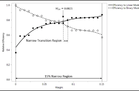
26 multiple 𝑊𝑁 with very similar performance, another transition region on the narrow relative

efficiency plot is identified. This transition region will be called the narrow transition region. The

𝑊_𝑁 with the smaller difference between 𝐷_𝑒𝑁 _{and 𝐷}

𝑒𝐵 is selected as the 𝑊𝐶𝑂. Figure 11 illustrates

this process using a narrow relative efficiency plot.

Figure 11: Illustration of true 𝑾_𝑪𝑶 selection

This process is repeated for each model configuration tested. For more information

regarding this algorithm, refer to Burke et al. (2017).

4.1 Estimating 𝑾_𝑪𝑶 using fitting techniques

In this section we describe the need to find the 𝑊_𝐶𝑂 algorithmically. Section 2.2 showed

that a single instance of Burke’s algorithm did not provide an acceptable compromise optimal

design. Section 4 showed that a better compromise design could be generated with a second

27 We propose an estimation method which provides an acceptable compromise optimal design

with only one instance of Burke’s algorithm. First, the techniques are presented with some

example graphs. Second, the selection criterion is presented. Finally, the best suited fitting

technique is presented.

The relative efficiency plots presented thus far show that identifying where a 𝑊_𝐶𝑂 may

appear is quite easy to do by finding the transition region. Data fitting techniques can harness

this visual intuition to provide a method for accurately estimating the 𝑊_𝐶𝑂 without a secondary

iteration of Burke’s algorithm at a narrow weight search region.

This research studied a variety of data fitting methods to estimate the 𝑊𝐶𝑂. The sets of

D-efficiencies (𝐷_𝑒𝑁) and DB-efficiencies (𝐷_𝑒𝐵) were fit separately to construct two model equations. These equations were solved for their intersection point to estimate 𝑊_𝐶𝑂. For each

fitting technique, two model equations are created per efficiency plot. Both equations take the

same form specified in Table 2. In one equation, the response variable 𝑦 = 𝐷_𝑒𝑁 and in the other

equation 𝑦 = 𝐷_𝑒𝐵_{. In both cases 𝑥}

𝑤 = 𝑊𝑁.The various fitting techniques used in this research

are summarized in Table 2. Some techniques fit models to all 21 weights, while others

28

Table 2: Summary of Fitting Techniques Tested

Fitting Technique Name # Weights Fitting Model Equation Polynomial (Degree = 2) 21 𝑦 = 𝛽0+ 𝛽1𝑥𝑤+ 𝛽2𝑥𝑤2+ 𝜀

Polynomial (Degree = 3) 21 𝑦 = 𝛽0+ 𝛽1𝑥𝑤+ 𝛽2𝑥𝑤2+ 𝛽3𝑥𝑤3+ 𝜀

Polynomial (Degree = 4) 21 𝑦 = 𝛽₀+ 𝛽₁𝑥_𝑤 + 𝛽₂𝑥_𝑤2+ 𝛽₃𝑥_𝑤3+ 𝛽₄𝑥_𝑤4+ 𝜀

Log Transform 21 𝑦 = 𝛽₀+ 𝛽₁𝑙𝑜𝑔(𝑥_𝑤) + 𝜀

Sqrt Transform 21 _{𝑦 = 𝛽0+ 𝛽1√𝑥𝑤 + 𝜀}

Linear 2 𝑦 = 𝛽₀+ 𝛽₁𝑥_𝑤+ 𝜀

Linear 4 𝑦 = 𝛽₀+ 𝛽₁𝑥_𝑤+ 𝜀

Polynomial (Degree = 2) 3 𝑦 = 𝛽₀+ 𝛽₁𝑥_𝑤+ 𝛽₂𝑥_𝑤2+ 𝜀

Polynomial (Degree = 3) 4 𝑦 = 𝛽₀+ 𝛽₁𝑥_𝑤+ 𝛽₂𝑥_𝑤2_{+ 𝛽}

3𝑥𝑤3+ 𝜀

Log Transform 5 𝑦 = 𝛽₀+ 𝛽₁𝑙𝑜𝑔(𝑥_𝑤) + 𝜀

Log Transform 6 𝑦 = 𝛽₀+ 𝛽₁𝑙𝑜𝑔(𝑥_𝑤) + 𝜀

Sqrt Transform 3 _{𝑦 = 𝛽0+ 𝛽1√𝑥𝑤 + 𝜀}

Sqrt Transform 4 _{𝑦 = 𝛽0+ 𝛽1√𝑥𝑤 + 𝜀}

Figure 12 shows two examples of fitting techniques considered. On the left, a linear

regression equation with 2 weights and on the right, a linear regression with 4 weights

surrounding the transition region.

Linear (2 Weights) Linear (4 Weights)

a) _b)

Figure 12: Linear Regression fitting technique

Each regression technique is evaluated based on two criteria. The first is deviation of the

29 between 𝐷_𝑒𝑁 and 𝐷_𝑒𝐵 from the narrow relative efficiency plot, as discussed Section 4. This is

referred to as the true 𝑊_𝐶𝑂, however it should be noted this is just the closest observed 𝑊_𝑁 to our

ideal. Section 5 provides further discussion on this topic. The estimated 𝑊̂_𝐶𝑂 for each method are

compared to the true 𝑊𝐶𝑂and an error is calculated as,

𝐸𝑠𝑡𝑖𝑚𝑎𝑡𝑖𝑜𝑛 𝐸𝑟𝑟𝑜𝑟 = 𝑊̂_𝐶𝑂− 𝑊_𝐶𝑂 (6)

The second comparison criterion is the simplicity of the using the technique for the

practitioner. Using these criteria, we propose a best practice methodology for estimating the 𝑊𝐶𝑂

in practical applications.

All of the fitting techniques listed in Table 2 were used to estimate the 𝑊_𝐶𝑂. The accuracy

of each method is presented as box plots shown in Figure 13. The vertical line at zero indicated

the target 𝑊_𝐶𝑂 value, or a perfect prediction.

Figure 13: Difference between estimated 𝑾𝑪𝑶 and true 𝑾𝑪𝑶 for each fitting technique

Accuracy of the techniques is determined by the techniques that produces estimation

error which is closest to zero. Precision is determined by the technique with the smallest

30 the 3rd _{degree polynomial linear regression model using a subset of 4 weights. This technique} had the smallest variance of error and a small positive bias (i.e. a mean slightly above zero). This

bias was the smallest of all of the techniques however. The methods using all 21 weight data

points generally performed poor, all possessing larger variance of error than the subset methods.

Other methods which performed well were the 2nd _{degree polynomial with 3 weights and the} logarithm transform of 𝑥𝑤 with 6 weights.

The second criterion used for the selection of the best fitting technique was the difficulty

of implementation. All of the techniques tested were available through the JMP software. Using

another software would have made these much more complicated. Fortunately, the techniques

tested are readily available within the JMP software. However subset techniques required a few

additional steps to complete.

The easiest techniques to implement were those which used all 21 weights. The different

regression techniques (polynomial, log(x) and sqrt(x)) can be simply toggled between in the JMP

software. The subset techniques were slightly more complicated, requiring the exclusion of some

points prior to the fitting technique. The subset techniques with 2 or more weights were the most

difficult to implement since it required the selecting weights based on the location of the

transition region. Techniques with 4 or more weights did not have this issue since all 4 weights

provides a weight range of at least [0 : 0.15]. This larger range allowed the included weights to

always begin at 𝑊𝑁 = 0 and extend positively. This was possible since all 𝑊𝐶𝑂values appeared

between 0 and 0.10 as discussed in Section 3.1. The process of excluding weights from the

31 their properties to ‘exclude’. Though a relatively simple process already, this was accelerated

through the use of a JSL script.

The technique with best accuracy (i.e. estimation error with a mean close to zero) is the

3rd _{degree polynomial with 4 weights. The easiest techniques to implement were the techniques} which used all 21 weights. The most accurate technique of these was the log(x) transformation.

The tradeoff in estimation error from the 3rd _{degree polynomial with 4 weights to the log(x)} transformation with 21 weights is significant in comparison to the marginal time saved by

avoiding to subset the weights. Based on these results, the 3rd _{degree polynomial with 4 weights} was identified at the best estimation method and is used exclusively for the remainder of this

research.

4.2 Experiment to Vary Model Configurations

In this section we describe the steps taken to investigate how different model

configurations impact the compromise optimal design and 𝑊𝐶𝑂. This section refers to the first

two process boxes of Objective 2 in Figure 10. First, we describe parts that make up a model

configuration. Second, we present the sensitivity experiments used to guide which model

configurations to test. Third, an example of how these model configurations are used in Burke’s

algorithm is presented.

The prior response models have shown to affect the results of optimal experimental

designs for both single and dual response designs by Johnson & Montgomery (2009). Thus, it is

important to study how these prior response models affect the 𝑊_𝐶𝑂. These prior response model

conditions include the prior response model structure, prior mean parameter value (𝜃_𝑛) and prior

standard deviation of the mean parameter value (𝜎𝜃𝑛). This research also studies the impact of

32 A prior response model structure provides a description of the terms included in the prior

response model. The prior response models in Equation 1 and 2 (found in Section 1 of this

thesis) are considered a main effects (ME) model structure since they include only main effect

terms (𝛽₁𝑥₁and 𝛽₂𝑥₂). Two other prior response model structures are studied in this research.

The main effects with two factor interaction (ME2FI) structure for the linear and binary case as,

𝑦2𝑁 = 𝛽0+ 𝛽1𝑥1+ 𝛽2𝑥2+ 𝛽12𝑥1𝑥2+ 𝜀 ₍₄₎

𝑦_2𝐵 = 1

1 + 𝑒−(𝜃0+𝜃1𝑥1+𝜃2𝑥2+𝜃12𝑥1𝑥2) (5)

and the main effects, two factor interaction and quadratic (ME2FIQ) structure for the linear and

binary case as,

𝒚_𝟑𝑵 = 𝜷_𝟎+ 𝜷_𝟏𝒙_𝟏+ 𝜷_𝟐𝒙_𝟐+ 𝜷_𝟏𝟐𝒙_𝟏𝒙_𝟐+ 𝜷_𝟏𝟏𝒙_𝟏𝟐_{+ 𝜷}

𝟐𝟐𝒙𝟐𝟐+ 𝜺 (𝟔)

𝑦3𝐵 =

1

1 + 𝑒−(𝜃0+𝜃1𝑥1+𝜃2𝑥2+𝜃12𝑥1𝑥2+𝜃11𝑥12+𝜃22𝑥22)

(7)

The D-Optimal design for the linear case depends on the prior response model, but not on the mean variance of the model parameters. The DB-Optimal design for the binary case depends on the prior response model as well as the distribution of the model parameters. In this research,

we assume the parameters are normally distributed and provide a mean and standard deviation of

the parameter for the binary model. The mean model parameters are denoted with 𝜃_𝑖. The

standard deviation of the mean parameters for the binary response model uses 𝜎_𝜃𝑖. The final

condition of interest is the number of trials available in the optimal design. This is denoted as

such or as (# 𝑇𝑟𝑖𝑎𝑙𝑠).

To properly test the effect of each of these conditions on the compromise optimal design

and 𝑊_𝐶𝑂 in this sensitivity analysis, these model configuration conditions were varied using a

fractional factorial design. There is one sensitivity experiment for each model structure, which

33 The responses collected are 𝑊𝐶𝑂, 𝑊̂𝐶𝑂, 𝐷𝑒𝑁 and 𝐷𝑒𝐵. Table 3 shows trials in the Main

Effects (ME) sensitivity experiment. This is a 2_𝑉5−1 design with 5 factors

(𝜃1, 𝜎𝜃1, 𝜃2, 𝜎𝜃2, # 𝑇𝑟𝑖𝑎𝑙𝑠) varied between the levels shown in Table 3. 𝜃1 is the prior mean

parameter of 𝑥₁, 𝜃₂ is the prior mean parameter of 𝑥₂, 𝜎_𝜃1 is the uncertainty of the prior mean

parameter (𝜃₁), 𝜎_𝜃2 is the uncertainty of the prior mean parameter (𝜃₂) and (# 𝑇𝑟𝑖𝑎𝑙𝑠) is the

number of trials allowed for the optimal design. The intercept term of the prior response model

(𝜃0 and 𝜎𝜃0) is held constant across all trials (𝜃0= 2 and 𝜎𝜃0 = 0.5) and therefore are not shown

as part of the model configuration. Since the prior mean uncertainty factors do not affect the D -Optimal design, these are not necessary for the continuous response. However, the mean

parameters and number of trials are varied as specified in the sensitivity experiments.

Table 3: Sensitivity experiment of Main Effects Only (ME) model structure

Factors Responses

𝜽𝟏 𝝈𝜽𝟏 𝜽𝟐 𝝈𝜽𝟐 # 𝑻𝒓𝒊𝒂𝒍𝒔 𝑾𝑪𝑶 𝑾̂𝑪𝑶 𝑫𝒆𝑵 𝑫𝒆𝑩

34 As example of the experiment in Table 3, the first row of Table 3. The settings of the first

run in this experiment is 𝜃1 = 6, 𝜎𝜃1 = 0.25, 𝜃2 = −2, 𝜎𝜃2 = 1, # 𝑇𝑟𝑖𝑎𝑙𝑠 = 16. The

configuration for the linear model is

𝑦_𝑁= 2 + 6𝑥₁− 2𝑥₂+ 𝜀 (8)

and the following binary model

𝒚𝑩 =

𝟏

𝟏 + 𝒆−(𝟐+𝟔𝒙𝟏−𝟐𝒙𝟐)

𝜽_𝟎~𝑵(𝟐, 𝟎. 𝟓𝟐_{) 𝜽}

𝟏~𝑵(𝟔, 𝟎. 𝟐𝟓𝟐) 𝜽𝟐~𝑵(−𝟐, 𝟏𝟐)

(𝟗)

This model configuration information can then be used in Burke’s algorithm (Section 4) and

fitting technique process (Section 4.1). The output of the algorithm and fitting technique

provides the 𝑊_𝐶𝑂, 𝑊̂_𝐶𝑂, 𝐷_𝑒𝑁 _{and 𝐷} 𝑒𝐵.

The sensitivity experiments for ME2FI (Table 7) and ME2FIQ (Table 8) are located in

the Appendix A. The ME2FI sensitivity experiment is a 2_𝐼𝑉7−2design with 7 factors. All the

factors from the ME sensitivity experiment remain with two additional factors. These factors are,

𝜃12, the prior mean parameter of 𝑥12 and 𝜎𝜃12, the uncertainty of the prior mean parameter (𝜃12).

The fractional factorial design requires 32 model configurations. The ME2FIQ sensitivity

experiment is a 2_𝐼𝑉11−6design with 11 factors, building off the factors included in the ME2FI

sensitivity experiment. The additional factors included are 𝜃11and 𝜃22, the prior mean parameters

of 𝑥₁₁ and 𝑥₂₂, respectively. As well as 𝜎_𝜃11and 𝜎_𝜃22, the uncertainty of the prior mean

parameters (𝜃11 and 𝜃22, respectively). This design also requires 32 model configurations. All

three sensitivity experiments are resolution 4 designs, meaning at least some interactions are able

35 The process for the ME2FI and ME2FIQ experiments is the same as detailed for the ME

sensitivity experiment. The results of all three sensitivity experiments are presented in Section 5.

5 Results

In this section, a report of the results of the sensitivity experiments is presented. Section

5.1 examines the quality of the fitting technique. Section 5.2 examines the effects of prior mean

parameters (𝜃_𝑛), prior mean uncertainties (𝜎_𝜃𝑛), and the number of trials on the dual response

compromise optimal design.

5.1 Impact of Estimation Error on Design Relative Efficiencies

This section compares the effectiveness of using our proposed fitting technique

estimation method to the exhaustive search algorithm for identifying the compromise optimal

design. The exhaustive search refers to the second iteration of Burke’s algorithm around the

narrow search region to find the true 𝑊_𝐶𝑂. First, the capability of the exhaustive search is

quantified. Second, the estimation error of the best fitting technique is compared to the

exhaustive search capability.

The exhaustive search method used in this research, although effective, did have

limitations. This research narrowed in on a 15% weight region to identify the 𝑊𝐶𝑂. This narrow

region with 21 iterations create weight increments of 0.0075. Once again, the true 𝑊_𝐶𝑂 is likely

not found, but the closest 𝑊_𝑁 is often very near. The precision of this 𝑊_𝑁 is calculated as the

average absolute difference between 𝐷𝑒𝑁 and 𝐷𝑒𝐵 at 𝑊𝑁 shown as

∑|𝐷𝑒

𝑁_{− 𝐷}

𝑒𝐵|

𝑘

𝑘

(10)

where 𝑘 is the number of total model configurations tested (80). The 80 trials are comprised from

36 at their designed resolutions. The ideal method would generate a value of 0, whereas the method

used in this research results in 0.033. This means that the true 𝑊_𝐶𝑂 identified in this research

creates a compromise optimal design which has only has an average difference between 𝐷_𝑒𝑁 _and

𝐷_𝑒𝐵 of 0.033.

The exhaustive search accuracy can provide perspective to the results seen by the

estimation method. With 95% confidence, the 3rd _{degree polynomial fitting technique with 4} weights provides a 𝑊_𝐶𝑂estimation error between -0.01685 and 0.02208. This metric is rather

meaningless without linking the impact of this estimation error on the resulting design

efficiencies. For this, the absolute efficiency difference (Equation 10) is calculated at weights

adjacent to the 𝑊_𝐶𝑂 (increments of 0.0075) and plotted in density plots seen in Figure 14.

Desirable values of the absolute efficiency difference (Equation 10) result in density plots that

are low in the plot area (each plot in the grid being assessed individually). Flatter, horizontal disc

shaped plots indicate lower variation around the observed absolute difference. The best values of

the absolute efficiency difference (Equation 10) are seen at a 0 deviation from the 𝑊_𝐶𝑂, this is

37

Figure 14: Absolute difference between Relative Efficiencies

Figure 14 shows that, in general, overestimating the 𝑊_𝐶𝑂 (plots to the right of center in

Figure 14) result in less impact on the final design than underestimating. This may suggest that

favoring a slightly positively biased prediction method could yield better results than an unbiased

method assuming equal variance. This bias appears only slightly in the ME structure, but it

becomes more pronounced in the ME2FI and ME2FIQ structures. However, this is may be a

result of the 𝑊𝐶𝑂 proximity to 0 in these configurations. When the 𝑊𝐶𝑂 is found close to zero, a

slight deviation towards the 0 weight causes much larger impact on design efficiencies (refer to

Figure 10 for visual). The result of this deviation is captured in the ME2FI and ME2FIQ plots

when the deviations are negative (shown by the tall skinny density plots). This is helpful to

understand as the practitioner because they can consciously decide to use a method which

38

5.2 Impact of Model Configurations on Compromise Optimal Designs

This section introduces the two prediction models used to study the sensitivity of the

model configurations. This explanation is supplemented with design plots overlaying contour

probability plots to provide a visual impression of each component of the model configuration.

The sensitivity analysis is comprised of two types of prediction models: One model to

predict the true 𝑊_𝐶𝑂 and a second to predict the relative efficiencies (𝐷_𝑒𝑁, 𝐷_𝑒𝐵). The first

prediction model uses the true 𝑊_𝐶𝑂 as the response. Recall that the value of the 𝑊_𝐶𝑂 represents

the amount of weight (𝑊_𝑁) given to the normalized D-Optimal design criterion (𝜑̃_𝑁) and its complement weight (𝑊_𝑁− 1), for the DB-Optimal design criterion (𝜑̃_{𝐵_𝑁𝑒𝑤}). These variables are combined in the desirability objective function created by Burke et al. (2017) as

𝝋_𝑵𝑩= (𝝋̃_𝑵𝑾𝑵_)(𝝋̃

𝑩_𝑵𝒆𝒘𝑾𝑵−𝟏) (𝟏𝟏)

Burke’s algorithm maximizes Equation 11, which provides the optimal designs discussed in this

thesis. Notice a larger 𝑊𝐶𝑂 (substitute for 𝑊𝑁 in Equation 11), corresponds to more weight

given to 𝜑̃_𝑁. Also recall that the 𝑊_𝐶𝑂value is the point which 𝐷_𝑒𝑁= 𝐷_𝑒𝐵. Therefore when

interpreting the prediction equations of the true 𝑊_𝐶𝑂, a larger 𝑊_𝐶𝑂 (or 𝑊_𝑁) suggests that more

weight on the normal criterion to reach a compromise and a smaller 𝑊_𝐶𝑂 requires more weight

from the binary criterion. This interpretation is important for understanding the impact of the

significant factors in the prediction model.

The key exception to be aware of is when the values of the factor levels are negative

numbers. This is the case for 𝜃2, 𝜃12 and 𝜃22. Here the positive and negative relationships are the

opposite. When the levels are positive, the low level is the smaller magnitude number. When the

39 (𝜃2, 𝜃12 and 𝜃22) are mean parameters of the model configuration. These represent the

incremental effect between the corresponding prior response model variables (𝑥₂, 𝑥₁₂ and 𝑥₂₂)

and the continuous (𝑦_𝑁) or binary response (𝑦_𝐵). The sign of the mean parameter simply

represents the direction of relationship with the continuous or binary response.

The second prediction model predicts the average relative efficiency at the true 𝑊𝐶𝑂 as

(𝑫̅𝒆 =

𝑫_𝒆𝑵+ 𝑫_𝒆𝑩

𝟐 )

(𝟏𝟐)

Equation 12 is necessary since 𝐷_𝑒𝑁 and 𝐷_𝑒𝐵 are not strictly equal at the 𝑊_𝐶𝑂 in practice, thus a

single 𝐷̅𝑒 is used as an estimation. Using 𝐷̅𝑒 as a response provides a secondary method for

observing the effect of 𝜃_𝑛, 𝜎_𝜃𝑛and # 𝑇𝑟𝑖𝑎𝑙𝑠 on compromise optimal designs. A larger 𝐷̅_𝑒

suggests that less compromise from each response is required to reach a design equally adequate

for both responses, otherwise called the compromise optimal design.

The two prediction models were developed using stepwise regression on data collected

from the sensitivity experiment to determine a best prediction model for both 𝑊_𝐶𝑂 (Equation 13)

and 𝐷̅𝑒 (Equation 14).

𝑌𝐷̅_𝑒 = 𝑓(𝜃1, 𝜎𝜃1, 𝜃2, 𝜎𝜃2, # 𝑇𝑟𝑖𝑎𝑙𝑠) + 𝜖 (13)

𝑌_𝑊𝐶𝑂 = 𝑓(𝜃₁, 𝜎_𝜃1, 𝜃₂, 𝜎_𝜃2, # 𝑇𝑟𝑖𝑎𝑙𝑠) + 𝜖 (14)

The stepwise regression selects the significant factors from all factors included in the

sensitivity experiments. Most factors which are found significant appear in multiple prediction

equations. However, each prediction equation does differ. These commonalities and differences

40 It is helpful to visualize the relationship of 𝜃_𝑛, 𝜎_𝜃𝑛and # 𝑇𝑟𝑖𝑎𝑙𝑠 to 𝑊_𝐶𝑂 and 𝐷̅_𝑒. Section 1

of this thesis introduced design plots overlaying contour plots to show how the binary response

affects the DB-Optimal design and compromise optimal design. The effect of model

configurations on compromise optimal design can be detected by the aforementioned 𝑊𝐶𝑂 and

𝐷̅_𝑒metrics, but also visually with these contour design plots.

First, we will consider the effect of manipulating the mean parameter values

independently and observe the resulting design contour plot. Figure 15 shows examples of

manipulating a main effect mean parameter (𝜃₁) value for Main Effects (ME) and an interaction

mean parameter (𝜃₁₂) for a Main Effects & Two-Factor Interaction (ME2FI) model structure.

Note that the shades represents the probability of the logistic response variable = 1, white areas

show where the probability < 0.10 and dark grey representing a probability > 0.90.

ME C o n fig u ratio n

𝜃1= 3 𝜃1= 6 𝜃1= 9

ME 2 FI C o n fig u ratio n

𝜃12= −1 𝜃12= −3 𝜃12= −5

Figure 15: Design Contour Plots at different levels of mean parameters

2 2

2

2

2

Probability of Response = 1