Efficiency in the higher education sector : a technical exploration, September 2013

(1)

BIS RESEARCH PAPER NO. 113

Efficiency in the Higher Education

sector: A technical exploration

(2)

EFFICIENCY IN THE HIGHER EDUCATION SECTOR:

A TECHNICAL EXPLORATION

Jill Johnes Geraint Johnes Department of Economics

Lancaster University LA1 4YX

E: [email protected] T: +44 (0)1524 592102 F: +44 (0)1524 594244

(3)

Executive summary

Costs incurred by a higher education institution in producing its output vary with the levels of output that it produces. They also vary with a number of other factors such as quality, student demographics, and the nature of the real estate. Even after allowing for all relevant factors, costs are likely to vary because institutions differ in their levels of efficiency. It is important to study differences in efficiency because this offers lessons about good practice that can lead to improvements in the performance of the higher education system as a whole.

Numerous studies analysing the costs of higher education institutions have been conducted, including many in the United Kingdom. Advances in statistical methodology have allowed these simultaneously to evaluate cost structures and institutional efficiency. The most recent studies, using latent class or random parameter stochastic frontier models, do this in a context that makes allowance for differences between types of

university (reflecting, for example, variation in student quality) that are not easily captured by the data.

In all exercises of this type, an important judgement call must be made concerning which of the factors affecting costs should be taken into consideration when determining

institutional efficiency. Clearly allowance should be made for differences in the level of output. Arguably allowance should also be made for differences in costs that are due to, say, the historical nature of an institution’s real estate, or to the role the institution plays in the widening participation agenda. In general, the more refined is the model of costs, the more efficient institutions appear to become, because the model contains more information that can be used to explain cost differences. There is no objective way of determining how much detail should be included in the analysis.

In this report, various stochastic frontier models are used to evaluate efficiency in English higher education institutions over the period 2003/04 to 2010/11, and over three sub-periods within that time frame. The stochastic frontier approach involves fitting a curve through data on costs and a variety of explanatory variables. This is not, however, a line of best fit; rather it is an envelope that defines an efficiency frontier – a curve that shows the lowest possible costs at which a given set of outputs can be produced. The position of this curve can then be used as a benchmark against which the efficiency with which each institution produces its output can be determined.

These are estimates of efficiency, and, like any other statistical estimates, are measured

with error. It is possible for one estimate to be different from another, but not significantly so in the statistical sense. In addition, there is no consensus about what value indicates an efficient or inefficient score. Consequently, the results should be interpreted with caution. The latent class stochastic frontier approach refines this method by separating the

(6)

allowing each institution’s efficiency to be assessed relative to other institutions of the same type.

An alternative to the latent class approach is to prescribe groups of institutions that, on a priori grounds, appear to share similarities with each other. The groups used in the recent HEFCE report on the impact of the HE reforms are used to define these clusters of

institutions.

The empirical work conducted in this project involves the evaluation of a large number of models of institutions’ costs, each of these models producing measures of institutions’ efficiency. The models range from a simple specification in which the explanatory variables include only linear terms in the outputs produced by each institution, through models that include further variables to capture factors such as widening participation and real estate characteristics, to models that include a rich variety of interaction terms designed to capture economies of scale and scope. The models are estimated first on the assumption that the same cost structure applies to all institutions, and secondly on the assumption that different groups of institutions exist for which cost structures may differ.

A key finding of the report is that, once differences between institutions are accounted for1, the variation in efficiency scores across institutions is greatly reduced, with a concentration of scores above 0.9 (where a score of one represents efficiency). Indeed, the relatively small number of institutions with low scores is exclusively made up of small and specialist institutions. The results do not, therefore, support the notion that substantial sector-wide gains could be made by using efficiency scores as a criterion for resource allocation. It may be argued that the more sophisticated models are the ones most appropriate for evaluating the efficiency of institutions, since they make most allowance for the different circumstances that might influence costs. Nevertheless there are drawbacks associated with using these models as a means of understanding costs in higher education. The greater sophistication of these models comes at a price. By increasing the number of explanatory variables used in the analysis, it becomes more likely that co-movement of some of the variables reduces the precision with which the impact of any one of them on costs is estimated. Moreover, the estimation of cost models that are specific to distinct classes of institutions involves, in effect, a reduction in the sample size used to estimate the model for each class. For these reasons, the simpler models reported here have considerable merit as means of understanding cost structures.

The analyses reported in this paper provide a useful starting point in understanding differences in efficiency across higher education institutions. The data on which they are based, however, are highly aggregated, and fail to capture the detail of how and why efficiency scores vary. A more in-depth analysis of institutions that achieve scores at either end of the distribution, such as via a case study approach, would be instructive as a

means of ascertaining the organisational factors underpinning efficient performance. This is likely to necessitate the collection of qualitative data of a kind that does not fit easily within the statistical approach adopted in this report.

(7)

1. Introduction

Under the new funding mechanism for higher education in England, many students will not pay off the whole of their debt within 30 years. The tuition fee charged by providers is not necessarily the same, therefore, as the amount paid by customers. The Resource

Accounting and Budgeting (RAB) cost of the student loans scheme is estimated to amount to around 35 per cent of the value of the loan book2, more than under the previous system, although there has been a simultaneous reduction in the amount of teaching grant, which, in effect, had a RAB cost of 100%. In addition, the fact that students do not make up-front payments reduces their price sensitivity. These factors have the potential to produce a market failure such that the usual competitive pressures fail to incentivise providers to become more efficient. Moreover, the government continues to subsidise both teaching and research, and has an interest in the efficient operation of all aspects of higher

education. An analysis of the cost structure and efficiency of higher education institutions (HEIs) is therefore of on-going interest and importance.

Extensive work has been undertaken on evaluating efficiency in the higher education sectors of various countries. Work in the United Kingdom (UK) is of particular relevance here (see, for example, Johnes and Taylor 1990; Johnes, J 1996; Johnes et al. 2005; Johnes 2008; Thanassoulis et al. 2011). Much of the literature on efficiency measurement has emphasised the statistical evaluation of costs (Cohn et al. 1989), since efficiency concerns how a given output can be produced at as low a cost as possible. Statistical and econometric techniques have been developed which allow efficiency to be evaluated for each institution. These statistical methods do not drill down into the detail of how

institutions do what they do3; rather they offer the analyst both an understanding of how costs are determined in higher education institutions as a whole, and a measure of the extent to which different institutions manage to produce their outputs efficiently. It allows an assessment to be made of the extent to which institutions differ in terms of their efficiency, and it also allows an analysis of changes in efficiency over time. At a higher level of abstraction, the method provides much the same input into benchmarking exercises as do more qualitative exercises, but it offers the advantage of a focus on the front-end activities of teaching and research. A number of studies exist which have adopted this general approach for UK higher education4 (Glass et al. 1995a; 1995b; Johnes, G 1996; Johnes 1997; 1998; Izadi et al. 2002; Johnes et al. 2005; Stevens 2005; Johnes et al. 2008b; Johnes and Johnes 2009; Thanassoulis et al. 2011).

2_{Announced by David Willetts at the Higher Education Policy Institute Spring Conference (15}th_{May 2013) -} see https://www.gov.uk/government/speeches/david-willetts-minister-for-universities-and-science-hepi-conference-speech.

3_{Unlike, for example, the Transparent Approach to Costing (TRAC).}

(8)

The purpose of this report is to undertake an empirical study of costs and efficiency in English higher education using data from 2003/04 to 2010/11. The report is in 6 sections of which this is the first. A review of empirical studies of costs in UK higher education is

presented in section 2. Section 3 examines linear and non-linear specifications of the cost function and the implications of particular choices. The methods of estimating cost

functions are considered in section 4 which also looks at how estimates of efficiency can be derived from the cost function. The empirical analysis using data, in turn, from 2003/04 to 2004/05, 2005/06 to 2007/08, and 2008/09 to 2010/11, is presented in section 5.

(9)

2. Review of the literature on costs

in higher education in the UK

There is now a considerable literature concerning the cost structure of systems of higher education, some of which also examines the efficiency levels of HEIs. The data underlying the empirical studies of costs in UK higher education span a period from the 1960s up to the early 2000s, and it is this literature which will be predominantly reviewed in this section. Additional details of the studies reviewed can be found in Appendix 1.

The first cost functions to be estimated and published for higher education in the UK relate to data from 1968 (Verry and Layard 1975) and include as outputs measures of both teaching and research. Six separate linear cost equations are estimated, one for each subject area: arts; social sciences; mathematics; physical sciences; biological sciences, and engineering. For undergraduate teaching, marginal costs are higher in the ‘laboratory’ science subjects than in the ‘classroom’ subjects such as arts, social sciences and

mathematics. The marginal cost of postgraduate teaching is higher than for undergraduate teaching, and (like undergraduate teaching) is more expensive in the sciences than in the arts.

Scale economies (which arise when an expansion of scale of production leads to costs rising less than proportionately with output) are observed in all subject areas (apart from physical sciences) but are significant only in the social sciences. In fact, the linear nature of the cost function makes it inevitable that there should be scale economies so long as there exist some fixed costs of provision – and in this respect the finding for physical sciences is somewhat curious.

(10)

Some of these issues are addressed, though not resolved, in a companion study (Verry and Davies 1976); but the seminal work by Cohn et al. (1989) was the real trigger for more sophisticated studies of costs of higher education in the UK which gradually got to grips with the shortcomings of these early models. Four studies, which use data for the pre-1992 definition of the university sector (Glass et al. 1995a; 1995b; Johnes, G 1996; Johnes 1998), address the issue of synergies in higher education production by using complex non-linear functional forms for the cost equations and by defining teaching outputs by broad subject area. Where undergraduate teaching is split by broad subject, the studies find that average costs of teaching within the arts are lower than within the sciences (at both undergraduate and postgraduate levels). For a given subject area, however, there appears to be little difference in the average costs of undergraduate compared to postgraduate teaching (Johnes, G 1996; Johnes 1998).

With regard to ray returns to scale – that is, returns to scale that arise from a simultaneous increase in all types of output being produced – there is evidence that scale economies are significant and unexhausted for the typical university (Glass et al. 1995a; 1995b; Johnes, G 1996; Johnes 1998). But the results regarding product-specific returns to scale – the returns to scale associated with an increase in one output only – are mixed (details can be found in Appendix 1) (Glass et al. 1995a; 1995b; Johnes, G 1996; Johnes 1998). Evidence regarding global economies of scope – the economies arising from producing all outputs together rather than separately – is also mixed. When teaching outputs are split by subject group in Johnes, G (1996) and Johnes (1998) we observe global economies of scope, but this contrasts with the finding of no significant scope economies when teaching output is aggregated across all subjects (Glass et al. 1995a; 1995b). This may be because studies where the outputs are more highly aggregated are, in effect, aggregating out the possibility of observing scope economies that exist at a finer level of analysis.

Two of these studies are the first to allow for inefficiency in the estimation of the cost function by using frontier estimation methods: stochastic frontier analysis (SFA) (Johnes, G 1996; Johnes 1998) - and data envelopment analysis (DEA) - (Johnes 1998)5. Efficiency of each HEI is measured on a scale of zero to 1 with the latter representing complete efficiency. The studies find that mean efficiency for the higher education sector as a whole is over 0.90 (using the DEA method). The estimates of efficiency derived from the two frontier estimation methods are positively correlated, although, at 0.133, the magnitude of the correlation coefficient is rather low, suggesting that the two frontier estimation methods provide different rankings of HEIs based on estimated efficiency. Any estimate of efficiency for an individual institution therefore needs to be treated with extreme caution.

The higher education sector in the UK saw major changes in its composition in 1992, when polytechnics were given university status, and later in 2003 when it was announced that Colleges of Higher Education would be allowed to apply for university status. Six studies have estimated cost functions from data referring to the extended higher education sector (Johnes 1997; Izadi et al. 2002; Johnes et al. 2005; Johnes et al. 2008b; Johnes and Johnes 2009; Thanassoulis et al. 2011).

(11)

For undergraduate teaching, average costs vary by subject and are highest in the sciences (or in medicine followed by other sciences where a more detailed subject split is made) and lowest in the non-sciences (Johnes 1997; Izadi et al. 2002; Johnes et al. 2005; Johnes et al. 2008b; Johnes and Johnes 2009; Thanassoulis et al. 2011). The cost of

postgraduate teaching is generally higher than undergraduate teaching in the sciences and non-sciences, but lower than undergraduate teaching in medicine (Johnes 1997; Izadi et al. 2002; Johnes et al. 2005; Johnes et al. 2008b; Johnes and Johnes 2009;

Thanassoulis et al. 2011), but no reasons are provided for why this might be the case. The findings regarding economies of scale and scope, from the studies based on the extended higher education sector, differ from the findings of the earlier studies. Ray

returns to scale are close to constant or decreasing for the typical university (Johnes 1997; Izadi et al. 2002; Johnes et al. 2005; Johnes et al. 2008b; Johnes and Johnes 2009)

implying, in the latter case, that expanding output leads to an increase in costs. Findings on product-specific economies of scale are mixed and depend on choice of data (single-year or panel data), definition of outputs, the functional form of the cost function and the estimation method. Global diseconomies of scope are a consistent finding in these later studies (Johnes 1997; Izadi et al. 2002; Johnes et al. 2005; Johnes et al. 2008b; Johnes and Johnes 2009).

Results regarding efficiency in the extended higher education sector also vary by choice of data and estimation method. Using only a single year of data, average efficiency for the sector as a whole is estimated to be around 0.88 (Izadi et al. 2002). This result, somewhat surprisingly given the variety of HEIs included in the 2002 study, is not too dissimilar to results based on only 50 pre-1992 HEIs (Johnes 1998). There is a considerable range in efficiency, however, from under 0.40 to 0.99, and this is likely a consequence of the diversity of the HEIs in the sample. Institutions at the lower end of the distribution of efficiencies tend to have characteristics that suggest that their relatively high costs (given output) are due to idiosyncrasies that are not adequately captured by the data on outputs, and the efficiency scores attached to these institutions therefore needed to be treated with caution.

Studies which use a panel of data over a number of years find that mean efficiency is generally lower than in the single-period models. The magnitude also varies by estimation method: mean efficiency across the whole sector is 0.69 on the basis of SFA (Johnes et al. 2005; Johnes et al. 2008b), 0.863 when DEA is used (Thanassoulis et al. 2011), and 0.753 in the case of a random parameter SFA model (Johnes and Johnes 2009). A simple SFA, unlike DEA and a random parameter SFA, does not make any allowance for each HEI to have a different set of objectives or mission. Thus any efficiency results derived using SFA should be interpreted with this in mind.

There is strong evidence that efficiency varies by HEI type. Colleges of higher education appear to be least efficient and post-1992 and some pre-1992 HEIs are typically the most efficient (Johnes et al. 2005; Johnes et al. 2008b; Johnes and Johnes 2009; Thanassoulis et al. 2011). The available software has not, however, allowed evaluation of the extent to which these differences are statistically significant.

(12)

students, input prices, and real estate costs. While one study finds that the proportion of students achieving first and upper second class degrees has a positive influence on both costs and on efficiency (Stevens 2005), student quality is generally not a significant determinant of costs (Verry and Davies 1976; Johnes et al. 2005; Johnes et al. 2008b; Johnes and Johnes 2009). It is possible that the random parameter specification used in some of these later studies already accounts for persistent quality differences across institutions and hence leads to the finding of insignificance of the quality variable.

Dummy variables such as a London dummy and an Oxbridge dummy, included in models to reflect, respectively, differences in input prices and costs of upkeep of ancient buildings, are not significant determinants of costs (Johnes et al. 2005; Johnes et al. 2008b; Johnes and Johnes 2009). Once again, these results may be a consequence of using a random parameter framework.6

Clearly much work has been undertaken on estimating the cost functions and efficiencies of UK HEIs. Many of the earlier studies restrict output to just teaching and research, are estimated on the basis of a restricted sample of HEIs, and do not allow for inefficiency in higher education production; indeed only four of all the studies reviewed include a

measure of the third mission outputs of universities, use data which reflect the current composition of the English higher education sector and use a frontier estimation method (Johnes et al. 2005; Johnes et al. 2008b; Johnes and Johnes 2009; Thanassoulis et al. 2011). Thus conflicts in findings from the different studies regarding, for example, average costs and economies of scale and scope, are not surprising.

The diversity observed in the UK higher education sector raises difficulties in estimation which have not, to date, been adequately addressed. Previous studies have examined costs and efficiency amongst pre-defined mission groups and have found differences between them (Johnes et al. 2005; Johnes et al. 2008b; Thanassoulis et al. 2011). But these studies are based on preconceived notions of how costs ought to vary. In a later study (Johnes & Johnes 2009), a random parameters approach is adopted which

acknowledges that each university varies in its mission and faces distinct circumstances affecting its costs, but which allows the data themselves (rather than the researchers’ preconceptions) to determine the nature of each institution – and hence what each institution’s cost function should look like. The random parameters frontier estimation model is an exciting development. By allowing parameters to vary across institutions, cost functions for HEIs that are clearly different from one another can be estimated in a single framework and without recourse to separate estimation for pre-determined groups of HEIs. The disadvantage is that the model can be difficult to fit; indeed such were the demands on the data in this particular study that some of the richness of the previous models was lost by amalgamating the medicine and science undergraduate teaching outputs, and by dropping the third mission output measure from the equation. The random parameters approach might also be viewed as being too permissive in that, in effect, it allows each institution to define its own mission.

6_{Work reported later in the present paper, which does}

(13)

3. Specification of the cost

function: linear versus quadratic

Costs typically increase as output increases. In many contexts, and certainly in the case of most HEIs, the output of each producer comes in a multiplicity of forms. Hence a HEI might produce graduates in a number of disciplines at a number of levels (such as bachelors, masters, doctorates), and might also produce research and engage in

knowledge transfer across various fields. Each of these distinct outputs has an impact on costs. Moreover, these costs are likely to differ across institutions that have different types of student intake, and are likely to vary according to the extent to which they produce outputs of different quality.

3.1 Linear specification

The simplest way to consider the relationship between costs and output is to suppose that each unit of each type of output adds a certain (fixed) amount to total costs. This approach is appealing in that it suggests a functional form for a cost equation that is particularly simple to estimate using statistical methods. That functional form is linear, and given by an equation such as

C =  + T + R (1)

where C denotes total costs and T and R respectively denote the quantity of distinct types of output being produced, say teaching and research. The ,  and  terms are known as parameters of the model, and they are estimated statistically.

The simplest way to do this is to conduct a least squares regression, using data for a cross-section or panel of institutions; in effect, this involves evaluating a line (or, strictly speaking, a plane) of best fit through a scatter plot of data in three dimensions – one dimension for costs, and one for each of the output variables. A more appropriate

estimation technique is the stochastic frontier approach (SFA), which, rather than providing the line of best fit, evaluates the envelope of cost below which a certain combination of outputs cannot be produced, however efficient the producer. In this context, a latent class estimator can be used to estimate a separate cost equation, if desired, for each group of institutions (assuming two or more groups). More discussion of estimation methods and the implications of choice of method for efficiency estimation are provided in section 4. Once the estimation has been conducted, it is straightforward to interpret  as fixed costs (the costs that would be incurred even if production of teaching and research were zero),  as the (marginal) cost associated with each unit of teaching, and  as the (marginal) cost associated with each unit of research. In the case of the latent class model, the

parameters ,  and  will be different for each of the classes – indicating that one group of institutions has different fixed costs to the other, and that the (marginal) costs

(14)

This specification of the cost equation has the considerable merit of simplicity. The model has few parameters, and this reduces the likelihood with which statistical problems will be met that hamper the estimation. This is a particularly important consideration if the models being estimated are rich in terms of the number of explanatory variables being considered as potential determinants of costs. Moreover, the estimated parameters from a linear specification lend themselves to straightforward interpretation.

The linear specification of the cost function allows a limited consideration of returns to scale. If  is equal to zero, then a given percentage increase in both outputs, T and R, leads to the same percentage increase in C, thus implying constant returns to scale. If, on the other hand,  is greater than zero, a given percentage increase in both outputs leads to a smaller percentage increase in costs. This is because, with the increase in T and R, fixed costs can now be spread over a higher number of units of output. In this case we observe increasing returns to scale. It is possible also to observe diseconomies of scale (where  is less than zero), though this would be somewhat counterintuitive in the case of higher education since it would imply that system-wide costs are minimised by organising provision through a large number of very small providers.

While the linear specification of costs can provide some information about returns to scale, however, the specification itself is clearly highly restrictive in this regard. If returns to scale are increasing for some level of output, then they must be increasing for every level of output. Likewise, if they are decreasing (or constant) for some level, they must be decreasing (or constant) at every level. This does not correspond to the conventional thinking that returns to scale are initially increasing but subsequently constant or

decreasing as output rises. Neither does it correspond to the stylised facts: while there are relatively few very small institutions in existence, the higher education system is not

dominated by a single very large institution, sweeping up all the available economies of scale. It seems more reasonable to consider a specification of the cost equation that is capable of accommodating both increasing and decreasing returns to scale at different levels of output.

3.2 Non-linear specification

The preceding points suggest that a nonlinear specification of the cost function might have merit, and this in turn raises the question of what type of nonlinear representation of the cost equation might be appropriate. One specification that has been particularly popular in the literature is the quadratic cost function7. Using the same two outputs as above, this has the form

C =  + T + R + T2_{+ R}2_{+ TR} ₍₂₎

The squared terms in T and R, and the interaction term (where T and R are multiplied) give this equation its quadratic (nonlinear) character. The equation has several appealing

(15)

properties. First, returns to scale can be different at different levels of output. Depending on the parameter values, it is possible for there to be economies of scale at low levels of output, and diseconomies of scale at very high levels of output, thus providing a rationale for the existence of institutions that are neither very small nor very large. Secondly, the interaction term allows for the possibility that the joint production of the distinct types of output under consideration can yield economies. These are known as economies of scope, or synergies. In an important sense, the (potential) existence of economies of scope explains the existence of organisations as we know them. In the case of HEIs, such economies might explain why research is conducted within the same organisation as teaching, why postgraduates receive their training in the same organisations as undergraduates, or why tuition and research in the arts are delivered in the same organisations as tuition and research in the sciences.

The quadratic function thus provides a much richer framework within which to analyse costs than does the linear function. Both are parametric, and therefore impose restrictions on the shape that the cost curve can take. But, since the quadratic nests the linear as a special case8, the quadratic function is clearly more general. It is important to note,

however, that increasing the number of output types has very different implications for the two types of specification. In the linear case, increasing the number of outputs by one leads to an increase of one in the number of terms on the right hand side of the equation. In the quadratic case, increasing the number of outputs by one results in an increase of 2+x in the number of parameters, where x is the number of output types. This means that, even when considering only a modest number of outputs, the specification of the quadratic cost function involves many terms on the right hand side of the equation. This can result in statistical problems owing to over-parameterisation and multicollinearity9. For this reason, the quadratic model is most suitable when a fairly parsimonious model is under

consideration.

A further characteristic of the quadratic model is that each output appears more than once in the set of explanatory variables, because it appears in squared and interaction terms, not just as a linear term. This makes the interpretation of parameters more difficult than in the linear model. It is, however, possible to extract information from the model about measures that are of policy interest, such as the (marginal and average) cost associated with the provision of each type of output.

Once the quadratic cost function has been estimated – using the same types of statistical methods as are used to evaluate the parameters of a linear function – it is straightforward to calculate the marginal costs associated with each type of output. This measure

indicates how much an extra unit of output adds to total costs10. In contrast to the linear case, however, where the cost function is quadratic the marginal cost will not be a

8_{If in the special case that the coefficients}__,__,__{in the quadratic model (equation (2)) are all zero, then} equation (2) simply becomes the linear model of equation (1) with =, =, and =. Thus equation (2) is said to ‘nest’ equation (1).

9_{Multicollinearity occurs when two or more of the variables on the right hand side of the equation are highly} correlated. It can lead to imprecise estimates of the coefficients of the model, with small changes in model specification often leading to large changes in the estimated impact of each variable on left hand side variable – costs in this case.

(16)

constant. It will depend on the level of output. Owing to the existence of the squared and interaction terms, the marginal cost associated with each type of output will vary with the amount of that output type and with the amount of other output types produced. Hence the quadratic form of the cost function allows the returns to both scale and scope to vary, depending on the output profile of an institution.

The average incremental cost (AIC) associated with the production of a particular output type can be calculated as the difference between total costs at the outturn level of output and the estimate of what total costs would be if none of the output type of interest were produced (all other outputs remaining equal), expressed as a proportion of the outturn level of that output type11.

11_{See Baumol}

(17)

4. Cost function estimation and the

measurement of efficiency

The previous section made allusions to various statistical methods for estimating cost functions (such as least squares regression, stochastic frontier analysis, and latent class models). The choice of estimation method implies assumptions regarding the efficiency of the group of organisations whose cost function is being estimated, and hence has

implications for the measurement of efficiency. This section examines the issues of cost function estimation and the measurement of efficiency in more detail.

Organisations of various types have a variety of motivations that lead them to seek to be efficient. In sectors characterised by intense competition, efficiency is a prerequisite of survival. Elsewhere, efficiency is needed in order to ensure that the objectives of the organisation can be maximised. Where organisations are funded, at least in part, by the public purse, government has a responsibility to the taxpayer to ensure that resources are used efficiently. Yet the evaluation of efficiency is not straightforward.

Efficiency refers to the process whereby inputs are converted to outputs. The ratio of the value of outputs to the value of inputs provides one means whereby efficiency can be measured, and requires knowledge of costs, outputs and the estimation of the cost function. Early cost function studies used simple least squares regression to estimate a line of best fit through the data. This approach calculates, over a number of organisations, the average value of total cost associated with producing a given level of output, and does not tell us how cheaply it is possible to produce that output. We know, because we can see it happening, that it is possible to produce the output more cheaply than the average. In analysing costs and efficiency, therefore, it is important that we should be able to identify an envelope below which it is technically impossible for costs to go. Rather than a line of best fit (which may be estimated by regression), we need to identify the position of a cost frontier, a cost curve that would typically lie below the best fit line.

In practice, the method used to estimate the parameters of the cost frontier involves a modification of the basic least squares regression method. In the least squares method, the residuals (the gap between observed values for each data point and the line of best fit) are required to follow a normal distribution with a zero mean. This means that the

observed values are as likely to lie below the estimated cost curve as above it, and that the sum of deviations below the line is as great as the sum of deviations above the line. This clearly violates the requirement that the line should represent a frontier. For a

stochastic frontier model12, the requirement that the residuals follow a normal distribution is replaced by a specification in which the residuals are made up of two components: one is normal, with zero mean, and is designed to capture measurement error; the second

12_{The stochastic frontier model was introduced by Aigner}

(18)

component is non-normal (usually a half-normal distribution is assumed13), and is designed to capture differences in efficiency across the observed units14. The effect of introducing this latter component of the residual is to shift the line so that it becomes a frontier rather than a line of best fit. The parameters of the model may be estimated using maximum likelihood techniques15. An advantage of this method is that it allows the

magnitude of the non-normal residual associated with each observation to be calculated; this may then be interpreted as a measure of efficiency. More commonly, the ratio of

predicted costs to the sum of predicted costs and the non-normal residual is used to define an efficiency score16_.

These measures of efficiency are interesting and are likely to be instructive at least inasmuch as they provoke questions. It should be remembered, however, that they are obtained from a statistical exercise in which a line (or plane) is fitted through data that do not allow a perfect fit. They are estimates of efficiency, and, like any other statistical

estimates, are measured with error. The efficiency estimate for each data point (in our case, each HEI) may be different from the estimate for other data points, but not (in the statistical sense) significantly so. Moreover, there is no consensus about the precise value an efficiency score should have in order for the unit to be deemed efficient or inefficient. As a result, caution is needed in their interpretation.

The stochastic frontier estimation approach (like earlier estimation methods) has the

underlying assumption that all production units under examination are directly comparable. It may be the case, however, that the cost associated with a given level of production may be higher in one organisation than in another for reasons that may reflect differences in the cost and production structures of different organisations rather than differences in

efficiency. For example, an organisation that enjoys the use of new, purpose-designed buildings may enjoy lower costs than one that uses antiquated accommodation. This may mean that the former is more efficient than the latter; but equally it may mean that the latter produces, as a by-product, intangible outputs (such as architectural heritage) which it is obliged to preserve. Likewise it is possible that different institutions differ in terms of the quality of students they can attract, and in the quality of graduates that they produce. It is important therefore to recognise the danger that the measurement of efficiency may be conflated with the issue of legitimate differences between organisations in cost and

13_{Alternative distributions for this error component include the truncated normal, the exponential and the} gamma distributions. The half-normal and exponential distributions have a mode at zero while the gamma and truncated normal models have a much wider range of distribution shapes. The parameters of the gamma and truncated normal, however, are much more difficult to estimate than for the half-normal and exponential distributions. While the values of efficiency scores can be sensitive to the precise distribution that they are assumed to follow, when observations are ranked on the basis of efficiency the rankings are usually not sensitive to choice of distribution (Coelli et al. 2005).

14_{It is possible to test whether the half-normal distribution of efficiencies (across all units) is significantly} different from zero using a statistic λ which is calculated from the variance of the random error component and the variance of the inefficiency component (Coelli et al. 2005). If λ is not significantly different from zero,

then there is no significant inefficiency component.

15_{Maximum likelihood estimation involves using an iterative procedure to find the parameters of a given} statistical model that maximize the likelihood of observing the particular set of data.

(19)

production structures. What constitutes legitimacy in this context inevitably involves a judgement call. It is possible, of course, to compare like with like, but someone has to make a judgement about how alike the members of each cluster of

organisations have to be in order to be deemed comparable.

These difficulties have been acknowledged by researchers for some time, and efforts have been made to develop methods that allow efficiency to be evaluated while ensuring that the organisations that are being compared with each other are indeed comparable. An important contribution to this research effort is the development of the latent class stochastic frontier model17. This is a statistical model that allows the analyst

simultaneously to estimate the parameters of the cost structures of two or more groups of organisations and to evaluate the efficiency of each organisation in each group, while also determining which organisations comprise the membership of each group.

At the same time, the position and shape of this cost frontier needs to be evaluated separately for each of a number of groups of organisations. This is in recognition of the fact that different groups of organisations face different challenges and have different missions. The structure of costs is not expected to be the same across all organisations, simply because the characteristics of these organisations vary widely. There may be good reasons to suppose that there are (say) two distinct groups – or what we might call latent classes – of organisations included within the data set. The analyst can then set up a

problem that can be solved to provide estimates of the position and shape of two cost curves – one for each group. Part of the solution of this model involves establishing which organisations belong in which latent class. The problem is solved using maximum

likelihood estimation methods (see footnote 15). To be clear, the estimation methodology simultaneously provides information about what organisations comprise which group and

provides estimates of the parameters of the cost equation for each group.

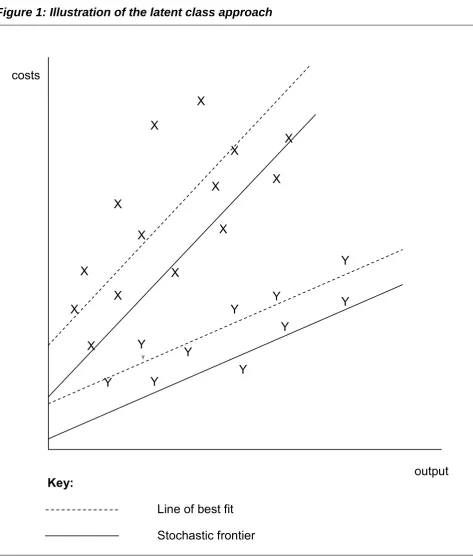
To summarize, it is possible to combine the stochastic frontier and latent class approaches so that (i) cost frontiers (or envelopes) are estimated (ii) yielding measures of the efficiency of each organisation in the data set and (iii) establishing which organisations belong in each of the latent classes or groups. This is illustrated in Figure 1. This shows a scatter plot of points, each of which describes the costs and output levels of a single observation. Each observation might represent a decision-making unit or organisation – for example a HEI. Where panel data are used, each observation might represent a particular

organisation in a particular time period. A straightforward latent class analysis of these data might involve the analyst in specifying that there are two18 different types of organisation in the data set. The latent class model therefore fits two lines to the data. These are shown by the two dashed lines. In fitting these two lines, the model also

determines which observations belong to which of the two latent classes – thus the model classifies some of the cost-output pairings into class X and some into class Y. These letters are shown as the data points on the diagram, but it should be emphasised that the observations are placed in these classes by the maximum likelihood algorithm used in the

17_{While the latent class model was introduced by Lazarsfeld and Henry (1968), the frontier version of the} latent class model was much later (Orea and Kumbhakar 2004; Greene 2005).

(20)

latent class estimation itself; the observations are not placed within one class or the other by the analyst.

The two dashed lines represent the best fit that is associated with the observations (given that there are two latent classes), but they do not represent the cost envelope faced by organisations within each of these two classes. To find these cost envelopes, the latent class method must be used alongside a stochastic frontier model. Doing this moves the lines down (and this is not necessarily a parallel shift). The resultant cost envelopes are represented by the solid lines. Note that, within each latent class, some observations lie below the cost frontier (because of the stochastic error component), but most lie above. The preponderance of observations above the frontiers represents inefficiency. The technique allows the efficiency of each observation to be evaluated by reference to its position relative to the frontier for the latent class to which the observation belongs19.

Caution should therefore be exercised when interpreting the results from a latent class model. In particular, while it is valid to compare HEIs within a group (because they are all being evaluated relative to the same frontier) it is not appropriate to make

comparisons across groups, since the estimated frontier may be different for each group20.

19_{This is done using a method developed by Jondrow}

et al. (1982).

(21)

[image:21.595.61.535.80.637.2]

Figure 1: Illustration of the latent class approach

X

X X

X

X X

X

X X

X

Y

Y Y

Y

Y _Y

Y costs

output Key:

Line of best fit

(22)

5. Empirical analysis

Several different specifications of the model of costs are reported in the tables that follow. These include both linear and nonlinear models; the former benefit from simplicity, but the latter have the advantage of allowing more sophisticated analysis of economies of scale and of scope. The simplest estimates reported below are based on an assumption that all institutions belong to a single class – that, while institutions might differ vastly in both scale and in the mix of outputs produced, the underlying technology is common, so that costs are determined in the same way in all institutions. The more sophisticated models assume that there are two or more latent classes, so that cost structures differ across these

classes.

5.1 Model specification

The explanatory variables in all models include a set of outputs and a number of controls. The outputs are: full-time equivalent (FTE) student numbers in each of four categories – undergraduates in medicine (UGMED), in other science (UGSCI), and in other subjects (which, for conciseness, are referred to as ‘arts’, though this set of subjects also includes humanities and social sciences - UGARTS) and the total number of FTE postgraduates (PG); research income (RESEARCH); and a measure of income from intellectual property (IPINCOME). This last variable is intended to proxy the output of third mission work

undertaken by institutions. The control variables, used in some models, are the number of students at the institution that come from neighbourhoods with low levels of participation in higher education (LOWPNO) and the area of the institution’s estate that has listed building status (LISTED). A binary variable is also included to identify the ancient institutions

(Oxford and Cambridge – OXBRIDGE), and, since the data used in the analysis are in the form of a panel of institutions over several time periods, year dummies are used to capture sector-wide changes over time. A complete list of variables with their precise definitions is provided in Appendix 3. All variables measured in monetary units are deflated to 2011 values by the Office for Budgetary Responsibility’s GDP deflator.

It is worth making a number of observations about the choice of explanatory variables used in the models. First, while undergraduates are disaggregated by broad subject area, the same is not done for postgraduates. Considerable efforts were made to evaluate models in which postgraduates are disaggregated into subject groups, but these proved to be unsuccessful, yielding results that were suggestive of statistical problems. Institutions that are major providers of postgraduate education in one area of their activity tend also to be highly active in training postgraduates in other areas. Hence several variables in the model were highly correlated with one another, thus making it impossible accurately to determine the effect on costs of each variable. This problem is known as multicollinearity, and it leads to imprecise estimates of the coefficients of the model, with small changes in model specification often leading to large changes in the estimated impact of each variable on costs. Aggregating across subjects at postgraduate level appears to mitigate this

(23)

Secondly, research income is used as a measure of research activity. This is standard in the literature, but is nonetheless worth commenting upon. The measurement of research undertaken by a university raises questions about how the quantity and the quality (or impact, perhaps) of research should be weighted. By using research income as a measure, these questions can be finessed. Income provides a measure of the valuation that is put on research by clients, and hence implicitly provides the appropriate weights on quantity and quality. It is recognised that the clients in this case are not necessarily all operating in competitive markets, but nonetheless the use of this measure offers (implicit) weights that are not arbitrary.

Alternative measures of research activity are available and have been considered for use in this study. Data on numbers of publications (PUBLICATIONS), and on the number of times work from each institution has been cited (CITATIONS), are available from the Web of Science. The correlation between research income, publications and citations measures of research activity is high, as is demonstrated in Table 1. Early experimentation with models similar to those reported below, using the publications and citations variables rather than research income, suggested that results are robust with respect to the choice of variable used to measure research activity. This being the case, and to be consistent with the received literature, the results reported below use the income measure of research.

Table 1: Correlation between various possible measures of research output (2008/09 to 2010/11)

Variable PUBLICATIONS CITATIONS

RESEARCH 0.973 0.776

PUBLICATIONS - 0.788

Thirdly, alternative measures of third mission activity are available from the Higher Education Business and Community Interaction Survey, and were considered for use in the present analysis. The number of people attending (ATEVENT), or the number of staff days involved in (EVENTS), events such as concerts, exhibitions, public lectures etc. at institutions are examples of such measures. Examination of the data on events reveals that the quality of the data is poor. Some institutions that are known to have arts centres report no attendance at events, for example. Moreover the data for single institutions often vary considerably, implausibly so, from year to year. This suggests that the interpretation of these variables differs both across time and across institutions. We experimented with inclusion of the variables (both individually and together) in early estimations, but the results confirmed that they were unfit for use in the statistical analysis. Therefore, this study only reports results where IPINCOME is the measure of third mission activity. Fourthly, the control variables used in the models reported below require some

justification. The character of an institution’s real estate is likely to be a major influence on maintenance costs. Two measures of the nature of the estate were considered as

candidate control variables in the current exercise. The first is the institutions’ self-reported figure for the estimated cost of upgrading their real estate to newly refurbished condition (UPGRADE). While superficially attractive, these data suffer a major drawback in the present context. Institutions which, over the period of analysis, engage in major

(24)

expected to have on costs. For this reason, the second variable – namely the area of the institution’s estate that is accounted for by listed buildings (LISTED) – is preferred. The variable UPGRADE was included in some early estimations but the results were

unsatisfactory (in that the coefficient was not significant and had a sign which did not accord with intuition), and hence our reported results only consider the impact of LISTED on costs.

Fifthly, the inclusion of a dummy variable for the ancient universities is worthy of discussion. It is not surprising to find that the cost structures of these universities are different from those of other HEIs. The nature of their estate, their organisational structures, the balance of their activities (with a relatively heavy concentration on postgraduate and research activities), and their positions in international rankings of universities all distinguish these universities from others in the country. One option would be to exclude them from the analysis, but this resulted in implausible values for some coefficients when estimation was based on all other observations, and in a latent class model which failed to converge. It appears appropriate therefore to employ an alternative approach of including a dummy variable to identify the Oxbridge institutions21.

Some further variables were considered for inclusion in the model, but do not appear in the preferred specifications reported below. Data from Unistats on graduate earnings, based on the Destinations of Leavers of Higher Education (DLHE) survey, provide a market based measure of the quality of institutions’ output (NMEAN) which is assumed to reflect inter-institution variations in quality of teaching output. There are various problems with including this variable in the cost equation. The data are based on survey data with different response rates for each institution. In addition, the data refer to graduates’ success in the labour market 6 months after graduation, and it is debateable whether this provides an adequate reflection of graduate quality. Finally, there is a problem with using average graduate earnings as a control variable in an equation which has total costs as the dependent variable. This would suggest that institutions’ fixed costs vary with quality (as measured by graduate earnings) but that variable costs do not. This is clearly

implausible. Nevertheless, graduate earnings were used as a control variable in some early specifications of the cost equation (not reported here), and consistently proved to be insignificant as a determinant of costs.

A further measure of quality that was considered for use in the analysis was institutions’ performance in the National Student Survey – specifically the percentage positive response to the question ‘overall, I am satisfied with the quality of the course’ (NSS). In common with the graduate earnings variable, this measure of quality suffers the drawback that its inclusion in a cost equation would imply that it can affect fixed but not variable costs. Its use as an explanatory variable in some specifications of the cost function

(25)

produced unsatisfactory results, typically leading to an estimated equation with efficiencies which have the wrong skew22.

Other factors which might be considered of interest, a priori, have not been included in the analysis because it has not been possible to obtain satisfactory measures. This is the case with, for example, the quality of student intake. We note, however, that the latent class approach adopted in some of the work which follows is designed precisely to allow for differences between HEIs which are not otherwise observed in the data.

We end this section by highlighting the points of original contribution of the empirical work reported below:

 We estimate cost equations for English higher education over a period of 8 years of data, and also for sub-periods of 2 and 3 years within that period. This is a considerably longer period than any used in previous literature: typically, analysis has been been based on one year of data, or, in the case of panel data studies, on a maximum of 3 years of data.

 We include a measure of third mission output. Attempts have been made to measure third mission in some previous work, but the variable used here is more appropriate than any previously used. In addition, we consider the interaction of third mission and research output in some models reported below, and this is new to the literature.  Undergraduate teaching is broken down into 3 subject areas (medicine, other sciences

and non-sciences). Previous studies have typically divided teaching only into two subject areas; where three groups have been used in previous studies the approach has not been combined with a third mission measure and its interaction with research. Separation of undergraduate teaching into this many groups poses challenges in estimation which will be discussed in the context of the results presented below.

 We investigate for the first time in the literature the effect of other possible determinants of costs, in particular, the effect of recruiting students from traditionally low participation neighbourhoods (LOWPNO), and the effect of having buildings with potentially costly upkeep (LISTED).

 We investigate the possibility that the cost function varies for distinct groups of

universities, as revealed by the data, using stochastic frontier latent class estimation. This is the first time this approach has been used in the context of English higher education.

(26)

 We compare the cost functions and efficiency derived from the latent class approach with the cost functions and efficiency estimated using pre-defined classes of ‘similar’ institutions. These pre-defined classes are the same as those used by the Higher Education Funding Council for England (HEFCE 2013).

5.2 Data

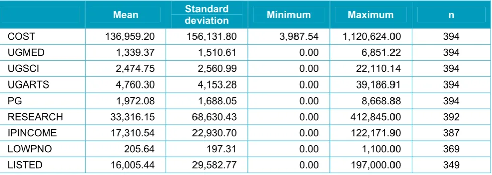
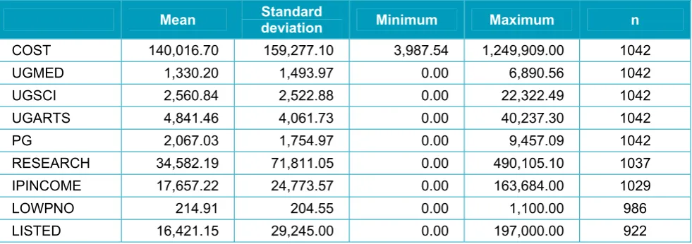
[image:26.595.55.545.517.691.2]

Summary statistics for the variables used in the models for each of the time periods are displayed in Table 2. It should be noted that values of n (number of observations on which the mean is calculated) vary because of missing data for some variables.

Table 2: Summary statistics for the data

a) 2008/09 to 2010/11

Mean Standard _deviation Minimum Maximum n

COST 156,943.20 178,620.10 5,424.49 1,249,909.00 387

UGMED 1,333.43 1,457.47 0.00 6,839.48 387

UGSCI 2,684.83 2,344.37 0.00 9,249.96 387

UGARTS 5,101.03 3,703.83 0.00 16,162.84 387

PG 2,229.55 1,890.64 0.00 9,457.09 387

RESEARCH 38,928.08 81,725.65 0.00 490,105.10 387

IPINCOME 19,958.34 28,859.26 0.00 163,684.00 384

LOWPNO 220.47 214.79 0.00 1,090.00 375

LISTED 16,624.64 28,023.97 0.00 182,536.00 367

b) 2005/06 to 2007/08

COST 136,959.20 156,131.80 3,987.54 1,120,624.00 394

UGMED 1,339.37 1,510.61 0.00 6,851.22 394

UGSCI 2,474.75 2,560.99 0.00 22,110.14 394

UGARTS 4,760.30 4,153.28 0.00 39,186.91 394

PG 1,972.08 1,688.05 0.00 8,668.88 394

RESEARCH 33,316.15 68,630.43 0.00 412,845.00 392

IPINCOME 17,310.54 22,930.70 0.00 122,171.90 387

LOWPNO 205.64 197.31 0.00 1,100.00 369

(27)

c) 2003/04 to 2004/05

COST 118,689.00 128,321.60 4,698.33 790,109.10 263

UGMED 1,305.93 1,523.77 0.00 6,890.56 263

UGSCI 2,487.89 2,713.90 0.00 22,322.49 263

UGARTS 4,546.28 4,407.67 0.00 40,237.30 263

PG 1,954.64 1,631.95 0.00 7,927.64 263

RESEARCH 29,874.27 59,394.44 0.00 311,924.80 259

IPINCOME 14,752.30 20,184.71 0.00 100,684.80 258

LOWPNO 219.59 199.40 0.00 975.00 243

LISTED 16,762.90 30,890.83 0.00 197,000.00 206

d) 2003/04 to 2010/11

COST 140,016.70 159,277.10 3,987.54 1,249,909.00 1042

UGMED 1,330.20 1,493.97 0.00 6,890.56 1042

UGSCI 2,560.84 2,522.88 0.00 22,322.49 1042

UGARTS 4,841.46 4,061.73 0.00 40,237.30 1042

PG 2,067.03 1,754.97 0.00 9,457.09 1042

RESEARCH 34,582.19 71,811.05 0.00 490,105.10 1037

IPINCOME 17,657.22 24,773.57 0.00 163,684.00 1029

LOWPNO 214.91 204.55 0.00 1,100.00 986

LISTED 16,421.15 29,245.00 0.00 197,000.00 922

[image:27.595.54.545.325.498.2]

5.3 Linear model over 3 time periods and for the whole time period

Table 3 reports the coefficient estimates obtained in a stochastic frontier regression of costs against linear terms in the various outputs and a set of control variables – including year dummies, an Oxbridge indicator, area of real estate comprising listed buildings, and the number of students originating from traditionally low participation neighbourhoods. The specifications of the model (and the models that follow) allow efficiency to vary across time for each institution in the data set. Costs are measured in thousands of pounds, so the coefficients on the student number variables each represent the sum (in thousands of pounds) that the marginal student adds to total costs. Hence, for example, one extra science undergraduate costs a typical university an extra £7,775 per year during the latest time period (measured at 2011 prices). It is readily observed that, within each of the (two or three year) time periods under investigation, the undergraduates that impose the

highest costs on institutions are those studying medicine, followed by those studying other sciences, followed by those studying other subjects. The higher costs of these subjects are recognised by the support given by HEFCE for band A and band B disciplines.

(28)

postgraduate provision involves one-to-one supervision), except undergraduate provision in medicine.

(29)

[image:29.595.54.548.104.472.2]

Table 3: Linear model with a complete set of controls

AICs 2008/09 to _2010/11 2005/06 to _2007/08 2003/04 to _2004/05 2003/04 to _2010/11

UGMED 13.48440 13.86610 9.74789 13.92710

UGSCI 7.77511 7.04032 5.60877 7.11761

UGARTS 4.57408 6.65664 3.95087 7.13533

PG 13.95320 9.40896 9.81821 12.21420

RESEARCH 0.81612 0.83696 1.18236 0.89197

IPINCOME 0.81920 1.15411 0.35017 0.81935

CONTROLS

2003/04 -2,485.99 -17,257.20

2004/05 -14,638.20

2005/06 -10,858.80

2006/07 3,640.36 -6,838.74

2007/08 10,429.90 -182.20

2008/09 3760.20

2009/10 -2,813.51 1437.09

2010/11 -4,070.18

OXBRIDGE 322,696.00 184,217.00 111,966.00 205,326.00

LISTED 0.31 0.25 0.22 0.12

LOWPNO -37.29 -33.06 -3.41 -28.63

CONSTANT -8,426.55 -39,195.80 -3,237.03 -42,488.50

Is λ significantly different from zero at

the 5% significance level? 23 YES YES YES YES

Notes:

1. Controls: LISTED; LOWPNO; OXBRIDGE; YEAR dummies.

2. Coefficients in bold are statistically significantly different from zero at the 5% significance level.

The universities of Oxford and Cambridge are distinctive owing to their antiquity,

organisational structures and academic orientation, and this is reflected in higher costs. Those institutions whose real estate includes a higher area covered by listed buildings typically have higher costs than others. Finally, those institutions that admit relatively high numbers of students from low participation neighbourhoods tend to have lower costs. This is, at first sight, a somewhat surprising result. The direction of causality, however, is open to debate: it may be that students from low participation neighbourhoods are attracted to institutions that have relatively low costs, possibly because of the type of subjects provided or because they undertake less research. The correlations between LOWPNO and,

respectively, UGMED, UGSCI, UGARTS and RESEARCH are 0.51, 0.67, 0.78 and -0.08 and are therefore consistent with this hypothesis. We do not investigate this further as it is not the main issue of interest.

(30)

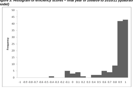
Estimation of the equations that comprise our models of costs also allows computation of efficiency scores for each institution. These are obtained from the one-sided residual in the stochastic frontier estimator, and may be expressed as the predicted value of costs divided by the predicted value plus the one-sided residual. A score of one thus implies efficiency, while lower scores imply the existence of some inefficiency. The distribution of efficiency scores suggests that some institutions are more efficient than others. To illustrate, the distribution associated with the 2008/09 to 2010/11 model reported in Table 3 is shown in Figure 2 (efficiency distributions associated with the other models in Table 3 are reported in Appendix 4.1). This indicates that the majority of HEIs have efficiency scores above 0.8, but that there is a noticeable tail of institutions which, on this measure, appear to be less

[image:30.595.69.525.344.651.2]

efficient. Some institutions have an efficiency score of less than zero. This is possible where the output levels of the institution are very low24, and indicates that the model of costs does not satisfactorily explain the relationship between costs and outputs for such small institutions. In Figure 2, the single observation at the bottom end of the efficiency distribution is the Rose Bruford College of Theatre and Performance which is a small specialist institution. As we shall see later, more refined models of costs tend to produce distributions of efficiencies that look rather different from those reported here.

Figure 2: Histogram of efficiency scores – final year of 2008/09 to 2010/11 (linear model)

In Table 4 we investigate the effect of excluding the control variables from the equation. The results are broadly similar, though some observations are warranted. First, there is a noticeable shift in the coefficient values between the two time periods reported in this table – and, indeed, for the 2005/06 to 2007/08 period, between the results obtained in this table

(31)

and those reported earlier. While, in the latest time period, it costs more to produce a marginal science undergraduate than an undergraduate in non-science subjects, the reverse is true in the earlier time period. The counterintuitive result obtained here for the 2005/06 to 2007/08 time period serves as a warning that some of the statistical results are not robust to minor changes in specification or modelling strategy.

Table 4: Linear model with a limited set of controls

AICs 2008/09 to _2010/11 2005/06 to _2007/08 2003/04 to _2010/11

UGMED 13.71790 14.17640 14.42160

UGSCI 7.34657 3.17296 3.89932

UGARTS 3.01348 6.04901 5.68941

PG 18.41520 13.46680 16.13060

RESEARCH 0.93983 0.93658 0.92238

IPINCOME 0.53013 1.11874 0.87065

CONTROLS

2003/04 -15,018.50

2004/05 -12,543.60

2005/06 -9,984.87

2006/07 5,220.86 -4,594.99

2007/08 10,904.60 1,229.65

2008/09 5,046.32

2009/10 -3,838.74 1,583.07

2010/11 -5,372.17

OXBRIDGE 309,483.00 186,112.00 205,629.00

CONSTANT -18,258.00 -44,053.60 -41,383.20

Is λ significantly different from zero at

the 5% significance level? YES YES YES

Notes:

1. Controls: OXBRIDGE; YEAR dummies.

2. Coefficients in bold are statistically significantly different from zero at the 5% significance level. 3. The 2003/04 to 2004/05 model does not converge.

(32)

5.4 Quadratic model over 3 time periods and for the whole time period

We now turn to consider the quadratic stochastic frontier model. The model includes as explanatory variables:

 linear terms in all variables

 squared terms in each of the student number variables, research, and income from intellectual property

 a full set of interaction terms between the student number variables, and between each of these and research

 an interaction term between research and income from intellectual property.

The model also includes a full set of controls. The estimated coefficients on the control variables are similar to those obtained in earlier models, and are not discussed further here.

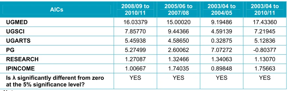
Rather than report the estimated parameters of the full quadratic model, which are difficult to interpret, Table 5 reports the average incremental costs (AICs) associated with each of the outputs. We use the definition of average incremental costs given in section 3.2 and evaluate at mean values of each of the explanatory variables. It is readily observed that these follow a similar pattern to that observed in the linear models described earlier – of undergraduates, students in medicine are the most costly, followed by those in other sciences. With the exception of the low estimate for non-science undergraduates in the 2003/04 to 2004/05 period, the estimates of average incremental costs look broadly plausible. The costs associated with postgraduates are lower than in the estimates

provided by the linear model, and those associated with research are higher. It is likely that collinearity between these two variables reduced the precision of the estimates. The

[image:32.595.51.551.580.737.2]

negative estimate of average incremental costs associated with postgraduate provision in the final column of the table is suggestive of statistical problems, and should be treated with scepticism. The relatively high values associated with undergraduate provision and, especially, third mission activity in this column indicates that multicollinearity could be adversely affecting the precision of these estimates.

Table 5: Quadratic model with a complete set of controls

AICs 2008/09 to _2010/11 2005/06 to _2007/08 2003/04 to _2004/05 2003/04 to _2010/11

UGMED 16.03379 15.00020 9.19486 17.43360

UGSCI 7.85770 9.44366 4.59139 7.21945

UGARTS 5.45938 4.58650 0.32875 5.12836

PG 5.27499 2.60062 7.07272 -0.80377

RESEARCH 1.27087 1.32466 1.34063 1.13070

IPINCOME 1.00667 1.74035 0.89848 1.75663

Is λ significantly different from zero

at the 5% significance level? YES YES YES YES

Note: