Coral assemblages and neutral theory

Full text

(1)Coral assemblages and neutral theory. Thesis submitted by Maria Ana Azeredo de Dornelas in June 2006. For the Degree of Doctor of Philosophy in Marine Biology within the School of Marine Biology James Cook University.

(2) STATEMENT OF ACCESS. I, the undersigned, the author of this thesis, understand that James Cook University will make this thesis available for use within the University Library and, via the Australia Digital Theses network (unless granted an exemption), for use elsewhere. I understand that, as an unpublished work, a thesis has significant protection under the Copyright Act and; I wish this work to be embargoed until November 2007. Maria Dornelas 27.06.2006.

(3) STATEMENT ON SOURCES DECLARATION. I declare that this thesis is my own work and has not been submitted in any other form for another degree or diploma at any university or other institution of tertiary education. Information derived from the published or unpublished work of others has been acknowledged in the text and a list of references is given. Maria Dornelas 27.06.2006.

(4) ELECTRONIC COPY. I, the undersigned, the author of this work, declare that the electronic copy of this thesis provided to the James Cook University Library is an accurate copy of the print thesis submitted, within the limits of the technology available.. _________________________ ______________ Signature. Date.

(5) Acknowledgments A number of people provided priceless support during this project, and I am grateful to them all. Firstly, I want to say a huge thank you to Sean Connolly. Sean was everything I could have wished for in a supervisor, providing invaluable guidance, constant availability, and freedom to disagree. Secondly, I am profoundly grateful to Terry Hughes for his precious advice, for giving me the opportunity to work with his incredible dataset, and for listening to my (sometimes) mad ideas. I want to thank the staff at the High Performance Computing Section, James Cook University, for all their assistance. Wayne Mallet, in particular, provided great support on using hydra and borg (the two super computers), and even translated some of my MATLAB code into C++, to speed the parametric bootstraps. I am very grateful to Brian McGill and Rampal Etienne for sharing their code and giving helpful advice on fitting neutral models. I also want to thank to Anne Magurran for friendly hospitality in her lab during the final stages of this thesis. I want to thank everybody that, over the years, participated in the Theoretical Ecology Discussion Group, as well as Laura Castell for listening to and/or reading several versions of this work and providing great feedback. A special thanks to Mia, Ailsa and Matt who also provided feedback, support and company out of the Friday meetings. I thank H. Cornell, R. Karlson and staff and students of the ARC Centre of Excellence for Coral Reef Studies for collecting, under the leadership of Terry Hughes, the dataset I used in Chapters 3 and 4..

(6) A huge thank you also to Abbi McDonald, Ailsa Kerswell, Alex Kerr, Andrew Baird, Jackie Wolstenholme, Marie Kospartov, Maria Joao Rodrigues, Mia Hoogenboom, Matt Kosnik, Naomi Gardiner and Scott Burgess for helping me collect the dataset I present in Chapter 5. They were not only far more efficient than I could have hoped for, but also lots of fun to work with. A special thanks to Jackie for sharing her precious coral identification skills with me. I’m also very grateful to Anne Hoggett, Lyle Vail, Marianne and Lance Pearce, for providing making the Lizard Island Research Station a great place to do fieldwork. I have no words to describe how grateful I am to Miguel Barbosa, for all the help he gave me along the way, and for being here for me always. A big, big thank you to Mum and Dad for everything, and to my Grandmother, who made me fall in love with biology. Finally, I am most grateful to the Fundação para a Ciência e a Tecnologia, Portugal, for supporting me during this PhD..

(7) Abstract. Abstract Neutral theory explains patterns of biodiversity based solely on speciation, demographic stochasticity, and dispersal limitation. The validation of this controversial theory depends on empirical support and it has been largely untested in marine communities. Coral assemblages have been repeatedly invoked as the animal communities most likely to conform to the assumptions of neutral theory. This thesis tested the hypothesis that neutral theory explains the macroecological structure of coral assemblages. Firstly, I assessed whether neutral models can accurately characterise coral species abundance distributions across multiple scales. Simulation-based and analytical neutral models were fitted to a hierarchical dataset of coral species abundance distributions from across the Indo-Pacific gradient of biodiversity. The dataset has three replicate habitats (slope, crest and flat), and three spatial scales (site, island and region). Both models exhibit significant lack of fit to empirical data at the site and island scales, but not at the region scale. The neutral model consistently underestimates the number of rare species, and overestimates the number of common species. Additionally, the neutral model fits coral abundance distributions less accurately than the poisson-lognormal at all scales. Using two formulations of neutral theory, and two goodness-of-fit tests, along with comparisons with the lognormal distribution, ensures that the inferences about coral assemblages and neutral dynamics are robust. Neutral model predictions are consistently and significantly different from observed coral species abundance distributions. Secondly, I developed a novel test of neutral theory that examines variability between communities of species relative abundances. In neutral communities, species.

(8) Abstract. relative abundances are determined by demographic stochasticity or “ecological drift”. Thus, communities diverge through time, and are expected to have low community similarity. In contrast, niche apportionment mechanisms have been invoked to argue that higher levels of community similarity should be observed under niche assembly than under neutral dynamics. These contrasting predictions provide an ideal opportunity to test neutral models against empirical data. Relative abundances of species across local communities differ markedly from neutral theory predictions: coral communities exhibit community similarity values that are far more variable, and lower on average, than neutral theory can predict. Surprisingly, empirical community similarities deviate from the neutral model in a direction opposite to that suggested in previous critiques of neutral theory. Instead, the results support spatio-temporal environmental stochasticity as a major driver of community structure at the macroecological scale. Thirdly, I unveiled a coral local community species abundance distribution. Community structure patterns are notoriously sensitive to sampling issues, and a comprehensive characterization of such patterns requires extremely large sample sizes. Consequently, the fit of biodiversity models to species abundance distributions, and parameter estimates in particular may be sensitive to sample size. To address these questions, over 44,000 corals were counted and identified to species at an exposed crest in Lizard Island, Great Barrier Reef. A neutral model was fitted to the species abundance distribution of the total dataset, and to sub-samples of various sizes. Parameter estimates and fit of the neutral model at different sample sizes were compared. The unveiled species abundance distribution appears to be multimodal. Parameter estimates are not affected by sample size..

(9) Abstract. These results strongly indicate that the limited suite of ecological and evolutionary processes included in neutral theory do not suffice to explain diversity patterns in coral assemblages. In combination, the three approaches included in this thesis suggest that neutral theory is most useful as a null model for community structure. Furthermore, the thesis highlights differences in species’ responses to environmental fluctuations as a potential major driver of species abundance patterns..

(10) Table of Contents. Table of Contents. Chapter 1: General Introduction ………………………….........….1 Chapter 2: A Review of neutral models…………………………...9 2.1 The origins of neutral models……………….……………….9 2.2 Neutral model assumptions………………………...……….11 2.3 Simulation neutral models…………………………………..13 2.4 Mean field neutral model…………………………...………15 2.5 Genealogical neutral model…………………………...…….16 2.6 Comparison of the three main models…………………..….18 2.7 Practical considerations……………………………….…….24 2.8 Conclusions…………………………………………...…….25 Chapter 3: Coral species abundance distributions: a multi-scale test of neutral theory……………………….……….27 3.1 Introduction…………………………………………..……..27 3.2 Methods………………………………………….………….30 3.3 Results………………………………………………………36 3.4 Discussion…………………………………….....………….42 Chapter 4: Neutral Dynamics and coral reefs: patterns of community similarity…………………………………46 4.1 Introduction……………………..…………………………..46 4.2 Methods………………………………….………………….48 4.3 Results………………………………………………………51 4.4 Discussion………………………………………………….59.

(11) Table of Contents. Chapter 5: Unveiling a coral species abundance distribution….64 5.1 Introduction……………………………………………..…..64 5.2 Methods…………………………………………..……...….68 5.3 Results………………………………………………………71 5.4 Discussion…………………………………….…………….84 Chapter 6: Conclusions…………………………..………..……….88 References………………………………………......………………92 Appendix I…………………………………………………………105 Appendix II…………………………...………………………..….142 Appendix III……………………………………………………….149.

(12) Table of Contents. List of Figures Chapter 2: Figure 2.1 – Species abundance distributions predicted by the Simulation Neutral Model and the Genealogical Neutral Model: the effect of m. Figure 2.2 – Species abundance distributions predicted by the Simulation Neutral Model and the Genealogical Neutral Model: the effect of J. Figure 2.3 – Species abundance distributions predicted by the Simulation Neutral Model and the Genealogical Neutral Model: the effect of θ. Chapter 3: Figure 3.1 – Comparison of parameter estimates with the Mean Field Neutral Model and the Simulation Neutral Model. Figure 3.2 – Frequency distribution of Log-Likelihoods from the parametric bootstrapping. Figure 3.3 – Deviations between observed species abundance distributions and fitted Simulation Neutral Model, Mean Field Neutral Models and poisson-lognormal. Figure 3.4 – Comparison between observed species abundance distributions and fitted Mean Field Neutral Models and poisson-lognormal. Chapter 4: Figure 4.1 – Frequency distribution of Jaccard and Bray-Curtis community similarities for neutral communities..

(13) Table of Contents. Figure 4.2 – Frequency distribution of Bray-Curtis community similarities for neutral communities: the effects of m and θ. Figure 4.3 – The effect of Jm on community similarity. Figure 4.4 – The effect of the number of turnovers on community similarity and species richness. Figure 4.5 – Comparison of observed and predicted community similarities. Figure 4.6 – Comparison between observed community similarities and neutral communities under multiple parameter combinations. Chapter 5: Figure 5.1 – Map of study site in Lizard Island. Figure 5.2 - Unveiling a coral species abundance distribution. Figure 5.3 – The contribution of non-crest species to a crest species abundance distribution. Figure 5.4 – Genealogical Neutral Model Log-Likelihood surfaces for a coral crest species abundance distribution I. Figure 5.5 – Genealogical Neutral Model Log-Likelihood surfaces for a coral crest species abundance distribution II. Figure 5.6 – Genealogical Neutral Model Log-Likelihood surfaces for a coral crest species abundance distribution III..

(14) Table of Contents. Figure 5.7 – Genealogical Neutral Model Log-Likelihood surfaces for a coral crest species abundance distribution IV. Figure 5.8 – The effect of sample size on neutral model parameter estimates. Figure 5.9 – Comparison between observed and fitted Genealogical Neutral model species abundance distributions I. Figure 5.10 – Comparison between observed and fitted Genealogical Neutral model species abundance distributions II. Appendix I Figure A.I.1 – Estimates of θ across habitats and biodiversity gradient Figures A.I.2-35 – Observed and fitted Simulation Neutral Model and Analytical Neutral Model species abundance distributions. Appendix II Figures A.II.1-7 – Genealogical Neutral Model log-likelihood surfaces for different sample sizes..

(15) Chapter 1: General Introduction. Chapter 1: General Introduction Understanding the processes that govern biodiversity has long been one of the central objectives of community ecology (Hutchinson 1959; Whittaker 1972; MacArthur 1975). Since effective conservation efforts depend on understanding how ecological processes affect community structure, there are now also pressing practical implications associated with this endeavour. These questions are more relevant than ever as diversity is currently being lost at a rate unprecedented in the last 65 million years (Chapin et al. 2000). Coral reefs in particular are increasingly threatened, and urgent measures are needed in order to ensure the sustainability of these ecosystems (Hughes et al. 2003; Bellwood et al. 2004). The main objective of this thesis was to contribute to the understanding of the mechanisms that determine coral community structure. Throughout this thesis the term community is defined as a group of species that are taxonomically similar and compete for resources (i.e., belong to the same trophic group) (Hubbell 2001). For example, on a coral reef, the corals and fishes belong to different communities according to this definition. Community structure, thus defined, refers to the patterns of diversity, and of species’ relative abundances. Diversity indices are often used to characterize community structure. These indices aim to summarize community structure taking into account both the number of species in the community and their abundance (Magurran 2004). Diversity, however, is not an univariate linear property of a community, and different indices measure different properties of community structure (Hurlbert 1971). Alternatively, analysing the distribution of species abundance can provide more detailed information about community structure than diversity indices do. Therefore, the analyses in this thesis. 1.

(16) Chapter 1: General Introduction. focus on patterns of species abundances, particularly on how they vary among locations, as descriptors of community structure. Two statistical distributions are particularly prominent candidates as good descriptive models for species abundances: the log-series and the lognormal. The logseries is derived from the negative binomial and accommodates a large number of rare species and a decreasing number of increasingly abundant species (Fisher et al. 1943). It arises as the result of random sampling from a community with heterogeneous species abundances (Fisher et al. 1943). The lognormal is a normal distribution in a log scale (Preston 1948). Statistically the lognormal arises as a consequence of the central limit theorem: many different random variables interacting multiplicatively are expected to generate lognormal distributions (May 1975). Preston (1948) also remarked that ecological data are usually a sample from a community, and we seldom have information about entire communities. Preston proposed that limitations of sampling would impose a “veil” on species abundance distributions, so that the rarest species would not be present in the sample. This veil would cause an apparent resemblance with a log-series distribution, which should disappear if sample size is increased. In fact, a sampling model for the lognormal (the Poisson lognormal) produces SADs that vary from log-series-like to lognormal-like depending on sample size (Pielou 1975; Lande et al. 2003a). Species abundance distributions (SADs) have remarkable similarities across ecological communities. Empirical data usually have SADs that resemble either logseries or lognormal distributions. Communities dominated by a few highly competitive species, with low to moderate diversity, or relatively small samples from a large community often have log-series SADs (May 1975; Hubbell 2001; Magurran. 2.

(17) Chapter 1: General Introduction. 2004). However increasing sample size often reveals an internal mode, as a lognormal-like distribution is unveiled. This “unveiling” has been demonstrated in communities as varied as, for example, birds (Nee et al. 1991), trees (Hubbell 1997b), estuarine fish (Magurran and Henderson 2003), and reef fishes and corals (Connolly et al. 2005). The two distributions are similar in most of their range (Hughes 1984), and therefore fitting a lognormal to samples that do not have an internal mode has been questioned (Hughes 1986). However, quantitative comparisons between the fit of the log-series and the sampling distribution from a lognormal to empirical data can still be made, even in the absence of an internal mode (Connolly et al. 2005). In general, species abundance distributions from a large variety of different communities seem to be well described by lognormal distributions. The regularity of patterns in species abundance distributions suggests that in general the same processes regulate community structure. The classical theoretical explanation for these patterns is based on species differences in niche (Hutchinson 1959; MacArthur 1960; Sugihara 1980; Tilman 1982; Tokeshi 1990). Each species is adapted to certain environmental conditions, and is most efficient (and therefore has a competitive advantage) in places where the environment is similar to its optimal conditions. The species that live in any particular location must compete for the resources available. Niche theory suggests that the fraction of resources each species consumes is related to its competitive ability (Tilman 1982) and each species consumes a fraction of the resources left available from its superior competitors. Finally if a species’ abundance is proportional to the fraction of resource it consumes, the distribution of species abundances can be predicted by this partition of resources (MacArthur 1960).. 3.

(18) Chapter 1: General Introduction. There are a number of ways that resources can be partitioned, which correspond to different predicted SADs. For example, if each species consumes a fixed fraction of the resources left available from its superior competitors (hierarchical model) the predicted SAD is a geometric series (Motomura 1932 in (Whittaker 1972). Alternatively, the broken stick distribution, which is similar to but more even than the lognormal, arises from the random partition of resources (MacArthur 1960). In this model the resource is partitioned at random, in S fractions of random size, where S is the number of species in the community. Finally, a hierarchical random partition of resources produces the lognormal distribution (Sugihara 1980). Resource partitioning in this model is often referred to as sequentially random, as species are sorted by competitive rank, and each species is sequentially allocated a random fraction of the resources left available by its superior competitors. This last model is particularly relevant, given the near-ubiquity of the lognormal distribution as a statistical description of empirical SADs. Numerous studies have provided evidence for niche theory. Examples include the comparison of empirical SADs with distributions obtained from the random assortment of species as well as with different niche models (Tokeshi 1990). More sophisticated studies examine multiple patterns, such as the proportionality between species abundances and the fraction of resources they consume when isolated (Tilman 1990; Harpole and Tilman 2006), or between species abundances and niche similarities (Sugihara et al. 2003). The mechanisms that promote species coexistence under niche theory have been thoroughly studied (Tilman and Pacala 1993) and niche assembly is generally considered to be an essential driver of community structure (Chesson 2000). Niche theory has, thus, been the paradigm of community ecology for the past half century.. 4.

(19) Chapter 1: General Introduction. In spite of this popularity there are some limitations to niche theory. Niche models are static and based on the abstract partitioning of resources. Ideally, theoretical models used to explain patterns of community structure should rest on basic ecological processes and allow exploration of community dynamics through time and space. Yet, developing dynamic models based on species niches has proven extremely difficult: even for communities of modest diversity, the models require far too many parameters (e.g. Schwilk and Ackerly 2005). An alternative explanation for community structure – neutral theory (Hubbell 1997b; Bell 2000; Bell 2001; Hubbell 2001) – has recently gained increasing attention. Neutral theory is based on demographic stochasticity and dispersal limitation. The neutrality assumption at the core of this theory means that all individuals, regardless of species, are demographically identical. This is in direct contradiction to niche theory, for which community structure is determined by species differences in resource use and local adaptation. Additionally, the neutrality assumption sits uncomfortably within community ecology, much of which is concerned with quantifying and explaining inter-specific differences in demographic rates, abundance, and distribution. Hence, it is not surprising that neutral theory is controversial (Abrams 2001; Brown 2001; Mazancourt 2001; Bengtsson 2002; Dial 2002; Silander 2002; Harte 2003; Ricklefs 2003; Chave 2004; Chisholm and Burgman 2004; Chase 2005; Gaston and Chown 2005). However, unlike niche models, neutral models are dynamic and explicitly incorporate fundamental demographic processes, such as births, deaths, and dispersal. Neutrality may be a reasonable simplifying assumption if inter-specific demographic differences are obscured by intra-specific variability, and thus species differences can be ignored when studying community structure. Most importantly, in spite of its simplicity,. 5.

(20) Chapter 1: General Introduction. neutral theory can produce community structure patterns that are surprisingly similar to empirical patterns (Hubbell 2001). Consequently, assessing whether neutral theory is capable of explaining observed community structure patterns is critical for the debate between niche and neutral theories. In this thesis, I test how well neutral theory can explain the community structure of scleractinian corals in the Indo-Pacific. As a highly diverse group with limited scope for resource partitioning within communities, scleractinian corals are ideally suited as a test case for neutral theory. The thesis starts with a review and comparison of the most prominent neutral models that have been explicitly fitted to empirical data (Chapter 2). I show that in spite of differences in ancillary assumptions (i.e., assumptions other than the “core” assumptions that species have identical resource requirements and demographic rates), the neutral models compared predict similar patterns. Thus, conclusions drawn from empirical tests of neutral theory are likely to be robust to the choice of which particular neutral model is used. Chapter 3 presents the first of three approaches used to test neutral theory: assessing the fit of neutral models to coral SADs across multiple scales, habitats and a biodiversity gradient. In this test I used an extensive data set of coral community composition that is housed at the ARC Centre of Excellence for Coral Reef Studies dataset (kindly provided by T.P. Hughes). The data include three habitats, and five regions distributed along a 10,000 km biodiversity gradient. In this Chapter, two neutral models are used to show that absolute goodness-of-fit tests indicate rejection of neutral theory as an explanation for coral community structure. Additionally, neutral models are rejected in a relative goodness-of-fit comparison with the lognormal.. 6.

(21) Chapter 1: General Introduction. Tests of macroecological theory based exclusively on curve-fitting to SADs are increasingly criticized as being relatively weak tests (McGill et al. 2006). Such tests do provide an important first test of the ability of a model to reproduce a pattern, but it is often impossible to use these results to link pattern and process, because several models can generate similar patterns (Magurran 2005). In particular, the superiority of the lognormal is difficult to interpret because, unlike neutral theory, it is not a mechanistic model. Therefore, in Chapter 4, I move beyond the analyses in Chapter 3 and present a novel test of neutral theory that is based on between community patterns. I analyse frequency distributions of community similarity and show that coral communities are more variable than neutral theory predicts. The nature of the differences between the data and the model predictions also highlight the role of environmental stochasticity in shaping reef corals community structure. The shape of SADs is highly sensitive to sampling effort. Extremely large sample sizes are needed to know the true underlying SAD of a community. Thus, the fit of models to these kind of data is likely to be affected by sample size. In neutral models, parameter estimates, and immigration rates in particular, may be affected by sample size. To address these questions, I collected the largest coral species abundance dataset from a single location. In Chapter 5, I unveil a local coral community’s SAD, and I determine whether neutral model parameter estimates are sensitive to sample size. The dataset reveals that increasing sample size does not unveil a lognormal distribution. Instead, the resulting distribution seems to be multimodal. Neutral model analyses also indicate that parameter estimates are robust to variation in sample size.. 7.

(22) Chapter 1: General Introduction. The thesis finishes with the overall conclusions and a brief discussion of the implications of the results for community ecology and conservation (Chapter 6).. 8.

(23) Chapter 2: A review of neutral models. Chapter 2: A Review of neutral models 2.1. The origins of neutral models Biodiversity neutral theory has its roots in population genetics. Neutral theory was initially developed to explain the dynamics of alleles with equal fitness consequences (neutral alleles) in population genetics (Kimura 1968; King and Jukes 1969). Most mutations are base substitutions that have little or no phenotypic effect, and hence a negligible influence on fitness. Such “neutral” mutations are thus not subject to natural selection, and genetic drift plays the principal role in evolution at the molecular level. Like the alleles in population genetics, in biodiversity neutral models, species are neutral. The neutrality assumption means that competition between individuals follows a lottery process that is independent of species identities. That is, all individuals in a community are competitively identical (use the same resources in the same amounts, and have the same demographic rates). In analogy with genetic drift, biodiversity neutral models propose that demographic stochasticity, in combination with dispersal limitation, drives community dynamics. Population genetic neutral models (Ewens 1972; Karlin and McGregor 1972; Watterson 1974) were first analysed in the context of community ecology in the 70’s (Caswell 1976; Hubbell 1979). Caswell (1976) advocated the use of neutral models as a scale of reference against which empirical patterns should be compared to estimate the effects of biological interactions on community structure. However, because immigrants were assumed to come from an infinite source of species, these models could not generate species abundance distributions (SADs) with the ubiquitous lognormal distribution. In contrast, Hubbell’s neutral model (1979) emphasized dispersal limitation and combined neutral dynamics with island biogeography theory. 9.

(24) Chapter 2: A review of neutral models. (MacArthur and Wilson 1967). This model generated lognormal-like SADs. However, most ecologists continued to focus on niche partitioning as an explanation for community structure (MacArthur 1960; Whittaker 1972; Sugihara 1980), and thus neutral models were largely ignored. It was not until recently that neutral models were proposed as a general explanation for biodiversity patterns (Hubbell 1997b; Hubbell 1997a; Hubbell 2001) and gained prominence. Hubbell’s (2001) claim that neutral theory was adequate to explain many empirical generalities in biogeography and biodiversity has caused a great deal of interest and controversy (Abrams 2001; Brown 2001; Mazancourt 2001; Bengtsson 2002; Dial 2002; Silander 2002; Harte 2003; Ricklefs 2003; Chave 2004; Chisholm and Burgman 2004; Chase 2005; Gaston and Chown 2005). Since then, there have been numerous theoretical developments and empirical tests of neutral models. In this Chapter I review the literature regarding biodiversity neutral models in general, and I compare the three main theoretical approaches to modelling neutral dynamics in particular. I start by discussing the assumptions of a broad suite of neutral models, and I highlight differences in ancillary assumptions that could potentially give rise to discrepancies in model predictions. Then I focus on the three main modelling approaches that can be, and have been, explicitly fitted to empirical data, and I describe them in some detail. To finalise I compare model predictions, to show that differences are minimal, and thus neutral models can be used interchangeably according to convenience. To conclude I discuss some practical considerations regarding the use of the different models.. 10.

(25) Chapter 2: A review of neutral models. 2.2. Neutral model assumptions There are currently several neutral models including both simulation-based (Bell 2000; Bell 2001; Hubbell 2001; Chave and Leigh 2002; Chave et al. 2002), and analytical models (Volkov et al. 2003; Etienne and Olff 2004; McKane et al. 2004; Etienne 2005; He 2005). By definition, neutral models assume that all individuals have the same probability of dying, producing offspring, speciating and immigrating from the metacommunity. Although per capita demographic rates are the same for all individuals in a community, species vary in their total mortality, birth and immigration rates: the more abundant a species is, the more likely it is that one individual of this species will provide a local birth or an immigrant, but also the more likely it is to die. In general, neutral models include two spatio-temporal scales: the metacommunity and the local community. At the metacommunity scale, speciation rate and the total number of individuals determine species richness and species abundance. At the local community scale, random deaths, births and immigration determine community structure. Both Hubbell’s (2001) simulation, and Etienne’s (2005) analytical neutral models have the additional assumption of community saturation, also known as the zero-sum assumption. This assumption states that every individual that dies is replaced either by a local birth or an immigrant, and therefore community size is constant. Because the number of individuals is unlikely to be constant in most communities, the applicability of neutral theory to unsaturated communities has been questioned (Silander 2002). However, this assumption is not present in some analytical neutral models (McKane et al. 2000; Vallade and Houchmandzadeh 2003; Volkov et al. 2003; McKane et al. 2004; He 2005). Comparing predictions made by. 11.

(26) Chapter 2: A review of neutral models. these different model versions should allow inferences about what, if any, is the effect of the saturation assumption. Neutral models also differ in terms of dispersal dynamics. In most simulation models local communities have complete mixing within them, but dispersal from the metacommunity is filtered through a migration probability (but see Chave and Leigh (2002) for a model with spatially explicit local communities). In contrast, it has been argued that analytical models can be conceptualised as a continuous landscape (Etienne and Alonso 2005), with dispersal limitation occurring at each point in space. Given the importance dispersal limitation plays in neutral models, it is important to understand the effects of these differences in dispersal dynamics for neutral theory predictions. Finally neutral models differ on the species abundance distribution (SAD) of the source pool of immigrants. Caswell’s neutral model has an infinite source of immigrant species (Caswell 1976). Bell’s neutral model (Bell 2000) as well as He’s neutral model (He 2005) sample immigrants from a distribution with a constant number of species and a uniform distribution. These three models do not make assumptions about how species originate, but most other neutral models (Hubbell 2001; Volkov et al. 2003; McKane et al. 2004) assume that species arise by point mutation (i.e. instantaneously with the initial abundance of one individual). This speciation mechanism generates a logseries metacommunity SAD from which immigrants are sampled. This speciation mechanisms has been criticized as being unlikely to be the predominant type of speciation, and for generating too many species with short life-spans (Ricklefs 2003). Other speciation mechanisms can be. 12.

(27) Chapter 2: A review of neutral models. used for neutral dynamics which generate different metacommunity SADs (Hubbell 2001). However, such formulations are not yet available as tractable models. The neutral models currently available can be classified into three main modelling approaches: simulation models, analytical models based on a mean field approximation, and analytical models based on a genealogical approach. These modelling approaches share the neutrality assumption, but, as discussed above, vary slightly in ancillary assumptions. Here I describe each approach separately, compare the patterns they predict, and discuss the advantages and disadvantages of using each modelling approach to test neutral model predictions.. 2.3. Simulation neutral models Biodiversity neutral models were firstly developed as simulation algorithms. There are several formulations that differ slightly in dynamics (Bell 2000; Bell 2001; Hubbell 2001; Chave and Leigh 2002; Chave et al. 2002). However, the most cited and commonly used simulation neutral model is Hubbell’s (2001). This is the simulation model I used in the following Chapters, and thus it is described here in detail (henceforth SNM). In the SNM, a local community is composed of J individuals. These individuals are initially randomly drawn from a metacommunity with Jm individuals. Metacommunity diversity is determined by both the per-time-step speciation rate (ν) and Jm. Under point mutation speciation, these two parameters always appear combined in the parameter θ (the “fundamental biodiversity number”).. 13.

(28) Chapter 2: A review of neutral models. If more than one speciation event is allowed to occur at each time step, θ is defined as: (2.1). " = 2Jm# (Hubbell 2001; Volkov et al. 2003). !. Alternatively if only one species can arise per time step, θ is defined as:. "=. $# (Jm %1) 1% $ #. (2.2). (Vallade and Houchmandzadeh 2003), where the per time step speciation rate (ν) ! relates to the per capita speciation rate (ν’). "=. "# 1$ " #. (2.3). In the SNM, θ determines the number of species in a sample of the ! metacommunity, because it corresponds to the probability that an individual belongs to a species not previously sampled. The metacommunity is the source of immigrants for local communities. The distribution of abundances in the metacommunity is similar to Fisher’s logseries, and, in practice, immigrants for the SNM are drawn from a large pool (relative to local community size) generated by a sampling algorithm (Ewens 1972; Hubbell 2001). Local community dynamics occur in discrete time. At each time step, D individuals randomly die. Each empty site is either occupied by an immigrant from the metacommunity with probability of immigration m, or by the offspring of an adult randomly chosen from within the community, with probability 1-m. In simulations,. 14.

(29) Chapter 2: A review of neutral models. SADs usually reach a noisy equilibrium after about 50 turnovers of the community (i.e., a total number of births that exceeds J by a factor of about 50) (McGill 2003c). Allowing enough turnovers for communities to stabilize is extremely important, as it affects not only the shape of SADs (McGill 2003c; Chisholm and Burgman 2004), but also the degree of divergence between communities (Maurer and McGill 2004). In this thesis, I adopt a conservative approach and run simulation models for 500 turnovers of the community (50 000 time steps with D = 1% of J). The shape of the SAD is determined by J, m and θ, and is not affected by the size of the metacommunity (Jm) or the number of individuals replaced at each time step (D).. 2.4. Mean field neutral model The first analytical approach to biodiversity neutral models to be developed applies mean field approximations to neutral models (McKane et al. 2000; McKane et al. 2004). Instead of examining the interactions among the species that compose a community individually, this approach assumes that a species interacts with all the other species in the community combined. Grouping all but the focal species greatly simplifies the dynamics involved, as only the interactions between the focal species and the rest of the community need to be taken into account, instead of the interactions between each pair of species in the community. Thus, grouping the effects of all the other species (using the “mean field approximation”) allows inferring an analytical expression for expected SADs. Several authors have followed this approach with equivalent results (McKane et al. 2000; Vallade and Houchmandzadeh 2003; Volkov et al. 2003; Alonso and McKane 2004; McKane et al. 2004). Here, and in subsequent Chapters, I use Volkov’s (2003) terminology (henceforth MFNM).. 15.

(30) Chapter 2: A review of neutral models. For the MFNM the probability that a species has abundance n (pn) is:. " J! $(% ) pn = S n!(J # n)! $(J + % ). x. & 0. $(n + x) $(J # n + % # x) ( e $(1+ x) $(% # x). #x" ) %. dx. (2.4). where θ , J and m are as defined for the SNM, S is the number of species, Γ is the ! gamma function, and γ = m(J-1)/(1-m) (Volkov et al. 2003). The expected number of species with abundance n is equal to pnS.. 2.5. Genealogical neutral model An alternative analytical approach returns to neutral theory’s roots on population genetics, specifically to Ewens sampling formula (Ewens 1972). It is based on developing the genealogical tree of the local community by tracing back each individual to its ancestor that immigrated from the metacommunity (Etienne and Olff 2004; Etienne 2005; Etienne and Alonso 2005) (henceforth GNM). In the GNM, the probability of observing a SAD in a sample from a local community with parameters. θ , m, J is:. P[D | ",m,J] =. J!. #. S i=1. ni #. J j=1. "S $j! (I) J. %. J A= S. K(D, A). IA (" ) A. (2.5). (Etienne 2005) where θ , m, J and S are as defined for the SNM and MFNM, ni is the ! number of individuals of species i, Φj is the number of species with abundance j. The notation (a)b is the Pochhammer symbol, or rising factorial, also denoted as ab which is defined as:. 16.

(31) Chapter 2: A review of neutral models. (a) b = a(a + 1)(a + 2)...(a + b "1) =. (a + b "1)! (a "1)!. (2.6). ! I is related to m in the same way as θ is related to ν’. I=. m (J "1) 1" m. (2.7). K(D,A) is. ! ni. S. K(D, A) = $ # a i =1 i=1. s(n i ,ai )(ai "1)! (n i "1)!. (2.8). where ai is the number of ancestors of species i, and s(a,i) is the absolute value of a ! Stirling number of the first kind (or the ith coefficient of the falling factorial ab):. a b = a(a "1)(a " 2)...(a " b + 1). (2.9). The sum of all the ai must equal A, the total number of ancestors in the local ! community. To fit the GNM, the combination of m and θ that minimizes expression (2.5) is found, rather than calculating log-likelihoods for each species abundance separately and then summing them. Although an analytical expression exists for the expected SAD in this model (Etienne and Alonso 2005), the expected SAD can also be obtained by using Hoppe urns to simulate samples from a distribution with a certain parameter combination (Etienne 2005). Hoppe urns work much like the metacommunity simulation algorithm in the SNM, where each individual in the sample is given a species label according to probabilities determined by θ and m. However, the GNM’s Hoppe urn represents a dispersal-limited community at equilibrium, rather than a fully mixed metacommunity. One advantage of the Hoppe. 17.

(32) Chapter 2: A review of neutral models. urn approach (over the analytical formula) is that, as with the SNM, a number of simulations can be run to estimate the variance of the number of species (across simulations) in each abundance class, as well as the mean.. 2.6. Comparison of the three main neutral models Discrepancies between predictions of different neutral models are of great importance, because they can affect the outcome of empirical tests. In particular the differences in ancillary assumptions previously discussed can potentially generate variations in predictions that are independent of the fundamental assumption of neutrality. Apparent discrepancies between different neutral model versions have previously been reported between the SNM and MFNM (Chisholm and Burgman 2004) and between the MFNM and the GNM (Etienne and Alonso 2005). Here I review the extent of these discrepancies, and show they can be resolved by small adjustments in the models. For completeness, and to illustrate the patterns predicted by neutral models, I present also a comparison of SADs generated by the SNM and the GNM. The SNM has been suggested to predict a lognormal-like distribution for parameter combinations (low m and medium to high θ) for which the MFNM predicts a low diversity flat SAD (Chisholm and Burgman 2004). This discrepancy is very important because the SNM’s ability to generate lognormal-like distributions has repeatedly been invoked as one of the strengths of neutral models (Hubbell 1997b; Hubbell 1997a; Hubbell 2001; Volkov et al. 2003). However, it seems that this apparent discrepancy is an artefact of failing to allow time for simulated communities to equilibrate. When the simulations described above are run for sufficiently many 18.

(33) Chapter 2: A review of neutral models. community turnovers, the SNM’s SADs do converge to the MFNM’s predictions of flat SADs (Chisholm and Burgman 2004). For extremely large J (~100,000), both the SNM and the MFNM do generate a lognormal-like SAD (Hubbell and Borda-DeAgua 2004). Hence, provided the distributions are allowed to stabilize, the SNM and MFNM seem to generate equivalent SADs. The MFNM has also been suggested to differ from the GNM. The MFNM is based on an approximation, which assumes Jm to be infinitely large. SADs predicted by the GNM have been reported to have fewer species than those predicted by the MFNM, when Jm < ∞ (Etienne and Alonso 2005). However, SADs are indistinguishable if Jm >> J (Etienne and Alonso 2005), which is the only realistic scenario, given that a metacommunity is composed of many local communities. Furthermore, Jm also does not affect within (Hubbell 2001) and between community patterns in the SNM (Chapter 5) as long as it is sufficiently larger than J. Thus, differences between the MFNM and the GNM caused by Jm are also easily resolved by adjusting the models to biologically meaningful scenarios. SADs predicted by the SNM, and GNM vary similarly with spatial scale and parameter values. A log-series distribution is predicted for the metacommunity (Hubbell 2001; Etienne 2005). For the local community, SADs vary considerably with the three parameters: m, J, and θ (Hubbell 2001; Fig 2.1, 2.2 and 2.3). Isolation decreases species richness (the height of the bars in SADs) and the proportion of rare and abundant species in local communities (the shape of SADs, Fig 2.1). As m decreases rare species go locally extinct, and abundant species become more abundant. This is reflected by the modal class moving to the right on a SAD plot. In particular, extremely low immigration rates (m = 0.0001) lead to communities with a. 19.

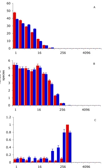
(34) 60 A. 50 40 30 20 10 0 1. 16. 256. 4096. 6. B. number of species. 5 4 3 2 1 0 1 1.2. 16. 256. 4096 C. 1 0.8 0.6 0.4 0.2 0 1. 16 256 4096 species abundance Fig. 2.1 - SADs predicted by the SNM (blue) and GNM (red) for a J of 1000, θ of 50 and m of 0.9 (A), 0.01 (B) and 0.0001 (C). Bars represent the mean of 100 simulations and error bars one standard error. 20.

(35) 1.2. A. 1 0.8 0.6 0.4 0.2 0 1. 16. 256. 4096. 1.2. B. number of species. 1 0.8 0.6 0.4 0.2 0 1 6. 16. 256. 4096 C. 5 4 3 2 1 0 1. 16 256 4096 species abundance Fig. 2.2 - SADs predicted by the SNM (blue) and GNM (red) for a θ of 500, m of 0.01 and J of 100 (A), 1000 (B) and 10000 (C). Bars represent the mean of 100 simulations and error bars one standard error. 21.

(36) 2.5. A. 2 1.5 1 0.5 0 1. 16. 256. 4096. 6 B. number of species. 5 4 3 2 1 0 1. 16. 10 9 8 7 6 5 4 3 2 1 0. 256. 4096 C. 1. 16 256 4096 species abundance Fig. 2.3 - SADs predicted by the SNM (blue) and GNM (red) for a J of 1000, m of 0.01 and θ of 5 (A), 50 (B) and 500 (C). Bars represent the mean of 100 simulations and error bars one standard error. 22.

(37) Chapter 2: A review of neutral models. single dominant species (Fig 2.1 C). However, the degree of isolation that leads to mono-dominance depends on J (Fig 2.2), as larger communities can sustain more species for a certain immigration rate. Additionally, higher diversity at the metacommunity scale (higher θ) leads to higher species richness at the local community scale (Fig 2.3). This effect is more pronounced for rare species, and thus, for constant m and J, θ affects not only the height of the distribution, but also the location of the internal mode. The SNM and the GNM modelling approaches generate similar predictions for most parameter values (Fig 2.1 to 2.3). The only apparent exception is for very low m and relatively high J (Fig 2.2 B, C), for which the GNM predicts a flat SAD with very few species, and the SNM a left-skewed lognormal-like distribution. This is analogous to the previously-reported differences between the SNM and the MFNM (Chisholm and Burgman 2004). However, the predicted abundance distributions for the SNM, like those shown in Fig. 2.2 B and C, are transient. When the SNM is run for more community turnovers, the differences are resolved because the SNM loses its lognormal-like shape as it tends to monodominance (Chapter 5). Nevertheless, this discrepancy highlights the importance of verifying that simulations have stabilized before making comparisons with empirical data. Thus, although SADs vary considerably with model parameters, the variability is consistent within these two model versions, and any differences are well within the variance inherent to simulations. As both the SNM and the GNM have been shown to be equivalent to the MFNM (see above), tests of neutral models using any of the three versions should yield similar results.. 23.

(38) Chapter 2: A review of neutral models. 2.7. Practical considerations The SNM relies exclusively on simulations. Therefore, this model version is the most susceptible to uncertainty, both in terms of the variation between simulation runs, and the stabilization (through time) of the patterns generated. When this model is fitted to empirical data, to reduce uncertainty related to simulation noise, abundances are usually classified into octaves (log2 classes of abundance). Multiple simulations are run, so that the expected SAD used for fitting uses the mean number of species (across simulations) in each abundance class to reduce susceptibility to simulation variation. When fitting the SNM to empirical SADs J is assumed to be equal to the sample size, and for each SAD, θ and m are sequentially estimated by Maximum Likelihood methods using Hubbell’s (2001) sequential estimation procedure. All of this, however, makes the SNM extremely computationally intensive. Nevertheless the SNM is the most flexible of all neutral models, as different ancillary assumptions can easily be incorporated with small changes to the simulation algorithm. Thus, it is extremely useful as a means to identify areas in which to invest analytical effort, and to examine combinations of assumptions that are not analytically tractable. It also facilitates quantifying the variance associated with neutral dynamics. Finally, some aspects of community structure can be readily examined by simulation (e.g. community similarity, as in Chapter 4), but cannot yet be examined with analytical versions of the theory. The MFNM and GNM avoid uncertainty in parameter estimates related to the stochastic fluctuations inherent to simulations. This increased accuracy allows them to be fitted to un-binned species abundances, instead of octave-classified abundances. Thus the MFNM and GNM provide more sensitive tests of goodness-of-. 24.

(39) Chapter 2: A review of neutral models. fit, and allow more accurate analyses of deviations between model predictions and observed SADs. Because the MFNM is essentially a sampling theory (Alonso and McKane 2004), when fitting this model J is the sample size, and m is the only estimated parameter, which is estimated by Maximum Likelihood methods. For every value of m attempted in the fitting procedure, pnS is solved for θ, by constraining the integral of the expected number of species with abundances between 0 and J so that it is equal to S. Thus, the MFNM has only one estimated parameter. However, because the integral in expression (2.4) must be solved numerically, this modelling approach is still extremely computer intensive and susceptible to numerical error (McGill et al. 2006), as well as difficult to implement. Furthermore, it is based on a approximation, and thus is not an exact analytical solution. In contrast, calculating the likelihood for the GNM, is far less computationally intensive than for the other neutral models. The GNM’s numerical efficiency allows more comprehensive explorations of likelihood surfaces, as well as efficient estimation of confidence intervals for maximum likelihood parameter estimates.. 2.8. Conclusions Biodiversity neutral models all share the fundamental neutrality assumption, although ancillary assumptions vary to some extent between different model versions. However, previous findings of differences between predictions of the models appear to be due to failure to reach equilibrium in simulation models. Thus the ”best” formulation of neutral theory to use can be based on its suitability for the aims of a particular study, rather than on the assumptions of the models. In Chapter 3, I used the SNM and the MFNM to test whether neutral models can predict coral SADs across. 25.

(40) Chapter 2: A review of neutral models. multiple scales, habitats and a biodiversity gradient. This study was completed before publication of the tractable form of the GNM (Etienne 2005). However, the results presented above strongly suggest that the findings in Chapter 3 would not have been different if I had used the GNM model instead. In Chapter 4, I examine patterns of community similarity, and I use the SNM because the analytical models currently do not make predictions regarding between community patterns. In Chapter 5, I exploit the computational efficiency of the GNM to examine parameter estimates for a coral community, and how these are affected by sample size. Again, the equivalence of the different neutral models shown in the present Chapter supports the robustness of the results in Chapter 5 to the choice of GNM.. 26.

(41) Chapter 3: Coral species abundance distributions – a multi-scale test of neutral theory. Chapter 3: Coral species abundance distributions – a multi-scale test of neutral theory 3.1. Introduction Neutral theory (Hubbell 2001) explains community structure based on the assumption that all individuals, regardless of species, are demographically identical. Hence, macro-ecological patterns are driven by speciation, demographic stochasticity, and dispersal limitation, with demographic and ecological differences between species having a comparatively negligible effect. The neutrality assumption contradicts much of classical ecological theory, which explains biodiversity and community structure based on local adaptation, and inter-specific differences in demographic rates, competitive abilities, and resource use (Hutchinson 1959; MacArthur 1960; Sugihara 1980; Tilman 1982; Tokeshi 1990). The assumption of neutrality has been branded as obviously “wrong” (Brown 2001; Mazancourt 2001; Baker 2002; Enquist et al. 2002; Norris 2003), because niche differences are likely to be essential to determine species coexistence (Chesson 1991). However, neutral theory should ultimately be judged based on its ability to explain empirical data. Coral assemblages are particularly suited to test neutral theory predictions. Most ancillary assumptions of neutral theory are appropriate for the biology of corals. In fact, the theory was originally proposed for tropical forests (Hubbell 1979; Hubbell and Foster 1986), which are often compared to coral reefs in terms of their high diversity. Neutral communities are, by definition, composed of trophically equivalent species, as is generally the case for coral assemblages. The life cycle of individuals in the neutral model includes an adult stage fixed in the same local community, and a dispersive reproductive stage, connecting different local communities into a. 27.

(42) Chapter 3: Coral species abundance distributions – a multi-scale test of neutral theory. metacommunity. This closely matches reef corals’ life cycle. Space (and the associated access to light) is the primary limiting resource, and there is a strong competitive advantage to incumbent space occupants. Therefore it is not surprising that coral assemblages have been repeatedly postulated as ideal for testing neutral theory predictions (Hubbell 1997b; Hubbell 1997a; Whitfield 2002; Chave 2004; Williamson and Gaston 2005). Neutrality, however, is a highly controversial premise, since there is little empirical evidence for competitive equivalence (Abrams 2001). However, equalising processes, such as priority effects and life-history trade-offs, have long been recognized as mechanisms of coexistence (Chesson 2000). From this perspective, it has been argued that neutrality approximates this kind of unpredictability in competitive interactions (Chave 2004), due, for instance, to intra-specific variability in competitive ability (Buss and Jackson 1979; Connolly and Muko 2003). Hence, neutrality has been argued to be a reasonable simplifying assumption when analysing community structure (Hubbell 2001). However, support for this proposition depends on the ability of neutral models to predict observed patterns. Species abundance distributions (SADs) are one of the most important ecological predictions generated by neutral theory (Chapter 1). The classical statistical model for SADs is the lognormal distribution, and it has been shown to provide good fit to coral abundance distributions (Connolly et al. 2005). Initial support for neutral theory was drawn from its apparent ability to characterise community structure in empirical communities better than the lognormal (Hubbell 2001; Volkov et al. 2003), although subsequent tests have generated contradictory results (McGill 2003c). In this. 28.

(43) Chapter 3: Coral species abundance distributions – a multi-scale test of neutral theory. Chapter I test the goodness-of-fit of neutral models to coral SADs, and compare it to the fit of a poisson lognormal (Connolly et al. 2005). Support for ecological hypotheses typically varies with scale (Levin 1992). This is particularly true for neutral theory, where defining the two spatio-temporal scales (local community and metacommunity) in ecological and evolutionary timeframes is crucial to ensure appropriate testing (Hubbell 2001; McGill et al. 2006). Local adaptation and habitat heterogeneity may be important at some scales but not others, and hence support for neutral theory may vary with the scale at which it is tested (McGill et al. 2006). However, most empirical tests of neutral theory have focused on a single spatial scale. Here I analyse coral SADs across multiple scales: with local communities examined at the scale of sites (1-2 km), islands (10-100 km) and regions (>1,000 km). In this Chapter I test whether neutral theory is consistent with observed coral SADs, and I compare neutral theory’s fit to the data with that of the lognormal. The tests are done at three different spatial scales, and for coral assemblages from across a 10,000 km biodiversity gradient, and three reef habitats (reef flat, crest and slope). Previous empirical tests using a single forest dataset have reached opposite conclusions depending on which model version and which statistical tests are used (McGill 2003c; Volkov et al. 2003). Hence, both the SNM (simulation neutral model – Chapter 2 (Hubbell 2001)) and the MFNM (mean field neutral model – Chapter 2 (Volkov et al. 2003; McGill et al. 2006)) are fitted to the data. I conduct a comprehensive analysis of relative abundance patterns, to understand how the absolute and relative performance of neutral theory depends upon spatial scale. I develop a new goodness-of-fit test for neutral theory that is based on the actual unit of. 29.

(44) Chapter 3: Coral species abundance distributions – a multi-scale test of neutral theory. ecological sampling (i.e., individuals), rather than on species (as conventional tests assume), and I apply it to these data. I also test the fit of the MFNM relative to the lognormal, using model selection statistics. The combination of fitting multiple neutral models, and of testing both absolute and relative fit at multiple spatial scales, and for assemblages from multiple habitats, and across a biodiversity gradient makes this study a particularly robust test of neutral theory.. 3.2. Methods 3.2.1. Data collection Coral species abundances were measured at several locations from across the Indo-Pacific to examine coral community structure patterns and to describe diversity and biogeographical trends. Sampling followed a hierarchical design with three spatial scales: regions, islands and sites. The five regions - Indonesia, Papua New Guinea, Solomon Islands, American Samoa and French Polynesia - are distributed along the Indo-Pacific gradient of coral biodiversity. Three high islands were selected in each region and four sites were chosen at each island (Karlson et al. 2004). Abundance of a species can be measured by the number of individuals, or by their biomass. In neutral models all individuals are implicitly assumed to be the same size, and hence the two measures are equivalent. However, in real communities, this is not the case, and different species can have dramatically different sizes. In fact the distribution of body sizes is one key macroecological pattern for which explanations are currently being sought (Brown 1999). This is particularly problematic in the case of colonial organisms, like corals, where individuals can be defined as a colony, or as the units that compose the colony. Furthemore, coral SADs using numbers of 30.

(45) Chapter 3: Coral species abundance distributions – a multi-scale test of neutral theory. individuals are strikingly different from SADs using colony cover (which is a proxy for biomass) (Connolly et al. 2003). In this study, each colony was counted as a single individual, so that all individuals originated from sexual reproduction, rather than by colony growth. This reflects more closely the type of lottery competition inherent to neutral models. At each site, all of the coral colonies intercepted by ten 10m long haphazardly placed transects were counted and identified to species. This was repeated in each of three reef habitats: slope, crest and flat using a total of 1800 transects. The different habitats were treated separately because their species composition is highly differentiated and neutral theory assumes homogeneous habitat. To generate island-level SADs, samples were pooled by summing the abundances of each species across the four sites on each island. Similarly, summing the abundances of each species across the 12 sites in each region created region-level SADs. A total of 60 site, 15 island, and 5 regional SADs were obtained for each habitat. 3.2.2. Testing the goodness-of-fit of the neutral model To determine if the neutral model can accurately describe coral SADs we tested the goodness-of-fit of the SNM and the MFNM to the data at each of the three spatial scales. The MFNM was fitted to each of the SADs by finding the value of m that maximizes the log-likelihood: J. LL = " Oi log(E i /S). (3.1). i=1. Where Oi is the observed number of species with abundance i, Ei is the ! expected number of species with abundance i, and S is the total number of species. Expected SADs were obtained using expression (2.4) in Chapter 2 (Volkov et al. 2003), using MATLAB code kindly provided by BJ McGill (McGill et al. 2006).. 31.

(46) Chapter 3: Coral species abundance distributions – a multi-scale test of neutral theory. Algorithms for fitting the MFNM are notoriously prone to numerical error, and, for this code, some numerical errors were present that led, in some cases, to dramatic underestimates of the probability of observing a species with a certain abundance. Therefore, I modified the code to use a slower, but more accurate function, in order to be able to confidently fit the model to species abundances rather than octave classified abundances. For this reason both the SNM and the MFNM were extremely computationally intensive (requiring several months on a supercomputer composed of 16 500 MHz MIPS R14000 processors and 68 400 MHz MIPS R12000 processors, housed at the High Performance Computing Section of James Cook University). I tested the goodness-of-fit of the neutral models by comparing the observed deviances with the corresponding expected deviances under the null hypothesis of neutral dynamics. Observed model deviance is calculated as: d = !2( LL ! LLs ). (3.2). where LL is the log-likelihood of the best fitted MFNM to the data, and LLs is the loglikelihood of the saturated model (Burnham and Anderson 1998). The saturated model follows the observed distribution exactly, that is the probability of observing a species with abundance i in the saturated model is equal to the proportion of species with abundance i in the data. Total deviance is the sum of deviances for all replicates at each spatial scale and each habitat. Expected deviance is estimated by implementing a parametric bootstrap: species are randomly sampled from a theoretical distribution of abundances with the same parameters as the data, and the model is fitted to these simulated samples. This procedure yields a null distribution of deviances. The proportion of bootstrap replicates with a deviance higher than the observed deviance (p) is a measure of the probability that goodness-of-fit of the. 32.

(47) Chapter 3: Coral species abundance distributions – a multi-scale test of neutral theory. model is acceptable. If p is low, then it is unlikely that the log-likelihood of the data is typical of a neutral community. Following convention, we take p<0.05 as our critical threshold value for rejecting the neutral model. Traditional goodness-of-fit tests for SADs, such as chi-square tests, treat species as the units of sampling, when in fact individuals are being sampled, and this is also true of the procedure described above. The SNM allows me to avoid this problem by simulating communities with the same number of sampling units (individuals) as the data. The SNM was fitted to each of the octave-classified SADs by Maximum Likelihood sequential estimation of θ and m (Hubbell 2001). I developed a method based on parametric bootstrapping to test whether the goodnessof-fit of the model to the data is worse than would be expected if a community were undergoing truly neutral dynamics. 1000 SNM datasets were simulated with the parameters estimated for the data. For each of the simulated datasets and each spatial scale the global goodness-of-fit (GGOF) was calculated as:. GGOF = " LLi. (3.3). i. where LLi is the log-likelihood of ith SAD. As a result, I obtain an expected ! distribution of GGOF statistics, under the null hypothesis that the data were generated by neutral dynamics. Thus, the proportion of simulated datasets with a log-likelihood more negative than the data’s (p) is an estimate of the probability that the goodnessof-fit of the data is consistent with a community undergoing neutral dynamics. Note that the goodness-of-fit statistic for the simulated data sets was calculated relative to the best-fit distribution for the empirical data, rather than from a best-fit calculated by fitting the SNM to each simulated abundance distribution separately (which would. 33.

(48) Chapter 3: Coral species abundance distributions – a multi-scale test of neutral theory. have been computationally prohibitive). The effect of this more exhaustive process would have been to increase the goodness-of-fit of the simulated data sets (i.e., the null distribution of fit statistics), without changing the fit of the actual data set. This would in turn increase the likelihood of rejecting the neutral model. Thus, this test is conservative with respect to rejecting the neutral model.. 3.2.3. Assessing the level of parameterisation of the MFNM To account for the effects of parameter uncertainty on the lack of fit, the MFNM was fitted separately for each site, and I also fit reduced parameter models. Specifically, the parameters were constrained to be constant for the entire dataset, for all sites within a region, and all sites within an island (Connolly et al. 2005). For each constrainment scale, the model was fitted by finding the value of m that maximized the sum of the log-likelihoods (expression 3.1) of all the sites included in that constrainment scale. Similarly, I fitted the MFNM for each island and for each region separately, and with constant parameters for the entire dataset and at the region scale, in the case of the islands. The relative fit of the different levels of parameterisation was compared using Akaike’s Information Criterion (AICc) (Akaike 1985):. AICc = !2 MLL + 2 p +. 2 p ( p + 1) n ! p !1. (3.4). Where MLL is the maximum log-likelihood, p is the number of parameters of the model, and n is the sum of the number of observed species abundances in each SAD. The estimated best model is the model with the lowest AICc.. To quantify the. uncertainty associated with model selection, Akaike weights were calculated:. 34.

(49) Chapter 3: Coral species abundance distributions – a multi-scale test of neutral theory. e !"i / 2 Wi = !" / 2 #e j. (3.5). where Δi is the difference between the AICc of model i and the lowest AICc of the models being compared. W estimates the probability that a model is the best among the models being compared. Aggregate comparisons were made by summing the MLLs and computing AICc and W using the corresponding (total) number of parameters and observations.. 3.2.4. Comparing the neutral model with the Poisson Lognormal To test the relative goodness of fit of neutral models in comparison with other available models, the fit of the MFNM was compared with the Poisson lognormal. The best level of parameterisation of the two models was used in this comparison, as the Poisson lognormal is best parameterised with constant parameters at the region scale (Connolly et al. 2005). The two models were compared using AICc, as described above.. Because the SNM was fit to binned abundances, its. likelihoods were not comparable to those of the other models, so it was not used in this analysis. Although the use of AICc for selection between different models is superior to approaches that rely on arbitrary P-values, its use is nonetheless somewhat controversial (Boik 2004). Therefore, I also quantify and examine the deviations between the data and the predictions of each model. For this analysis, I use both MFNM and SNM, as well as the poisson lognormal.. 35.

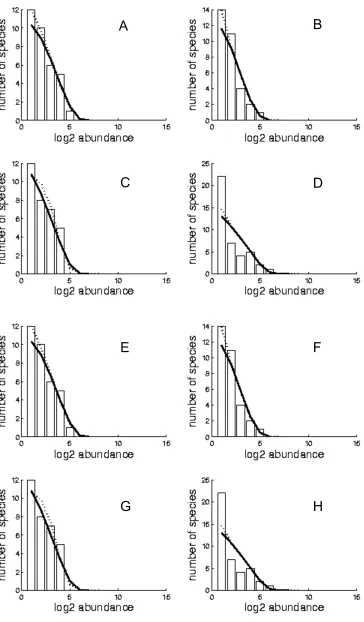
(50) Chapter 3: Coral species abundance distributions – a multi-scale test of neutral theory. 3.3. Results 3.3.1. Testing the goodness-of-fit of the neutral model Observed and fitted SNM and MFNM SADs are presented in Appendix I, Figs A.I.2-37. Parameter estimates for θ and m were similar for the SNM and the MFNM (Fig 3.1). Estimates of the diversity parameter θ increased predictably with increasing spatial scale, across the biodiversity gradient and the three reef habitats (Appendix I, Fig. A.I.1). θ varied between 1.3 (on a reef flat at a single site in Samoa) and 54.3 (on reef slopes at the regional scale in Indonesia). Estimates of θ with the MFNM were extremely well predicted by estimates with the SNM (Fig 3.1 A, R2 of 0.9914, 0.9949 and 0.9887 for the site, island and region scales respectively), although the MFNM had slightly higher estimates (see figure legend for regression equations). Estimates of m were consistently high. Over 50% were above 0.8, over 90% above 0.7, and all estimates were above 0.25. However, regressions between the estimates of m with the MFNM and the SNM had lower R2 (0.5599, 0.1692 and 0.695 for the site, island and region scales respectively), mostly because of the cases in which either one model or the other had m estimates below 0.8. The species parametric bootstrap analysis shows the MFNM exhibits significant lack of fit at the site and island scales (p < 0.001 in both cases). In contrast, at the region scale, the goodness-of-fit of both neutral models is low, but within expected values for a neutral community (MFNM p = 0.1625). Results from the individual parametric bootstrap are entirely consistent with the species parametric bootstrap. At the site and island scales the SNM exhibits significant lack of fit, whereas at the region scale goodness-of-fit is low, but within expected values (site and island p < 0.001, region p = 0.187, Fig 3.2).. 36.

(51) 60. A 50. MFNM. 40. 30. 20. 10. 0 0. 10. 20. 30. 40. 50. 60. SNM. 1 0.9. B. 0.8 0.7 MFNM. 0.6 0.5 0.4 0.3 0.2 0.1 0 0. 0.2. 0.4. 0.6. 0.8. 1. SNM. Fig 3.1 - Parameter estimates from the SNM and MFNMfor θ (A) and m (B). Blue diamonds represent sites, red squares islands, and green triangles regions. Best fitted regressions are respectively θMFNM= 0.9914*θSNM+1.3857 and mMFNM=1.7402*mSNM0.6016 at the site scale, θMFNM= 0.9949*θSNM+0.0670 and mMFNM=0.4502*mSNM+0.5549 at the island scale and θMFNM= 1.0321*θSNM+0.3966 and mMFNM=2.2053*mSNM-1.0304 at the region scale. See text for R2 values. 37.

(52) 0.1. A. 0.08 0.06 0.04 0.02 0. proportion of datasets. 0.14. B. 0.12 0.1 0.08 0.06 0.04 0.02 0 0.14 0.12. C. 0.1 0.08 0.06 0.04 0.02 0 -LL Fig 3.2 - Frequency distribution of negative Log Likelihood (-LL) of simulated neutral datasets at the site (A), island (B), and region (C) scales. The arrow marks the –LL of the empirical data. The –LL of the empirical data is much higher than any simulated datasets at the site and island scales, but not at the regional scale.. 38.

No results found