Characteristics of internal pressures in buildings with a dominant opening

Full text

(1)ResearchOnline@JCU. This file is part of the following reference:. Kim, Peter Young-Han (2012) Characteristics of internal pressures in buildings with a dominant opening. MEngSc thesis, James Cook University.. Access to this file is available from:. http://researchonline.jcu.edu.au/39261/ The author has certified to JCU that they have made a reasonable effort to gain permission and acknowledge the owner of any third party copyright material included in this document. If you believe that this is not the case, please contact [email protected] and quote http://researchonline.jcu.edu.au/39261/.

(2) Characteristics of Internal Pressures in Buildings with a Dominant Opening. Thesis submitted by Peter Young-Han KIM BESc in October, 2012. for the degree of Master of Engineering Science in the School of Engineering and Physical Sciences James Cook University.

(3) Acknowledgements 1 A c David Henderson and Dr. John Holmes. Their technical advice, guidance and critical feedback k throughout the course of this thesis were greatly appreciated. I would especially like to n acknowledge my primary supervisor John Ginger, who o always had an open door throughout this w thesis. l I acknowledge the Cyclone Testing Station (CTS) e for their support of this project d the CTS technical staff, their advice on through the use of equipment and resources, as well as g experimental setup was greatly appreciated. I also acknowledge technical staff from the e machine shop of the School of Engineering and Physical Sciences at James Cook University for m their help and advice. e n Finally, I thank my family and friends for their on-going support and encouragement. t s I would like to thank my supervising committee, Associate Professor John Ginger, Dr.. i.

(4) Abstract A building with a dominant windward wall opening will produce large internal pressures during a severe wind event and is a structural design criterion. Internal pressures were measured using a boundary layer wind tunnel for a series of windward dominant opening sizes, internal volume sizes and background building porosities. Internal pressures were also estimated using numerical simulations of the governing equation incorporating background porosity. The background porosity was represented as a single lumped porous opening. Results were presented in terms of a non-dimensional dominant opening size to internal volume parameter, and the lumped background porosity area to dominant opening area parameter,. .. The measured internal pressure results were compared with measured external pressures at the dominant opening. For the sealed building scenarios (no background porosity) but with a dominant opening, the mean internal pressure was equal to the mean external pressure, and the internal pressure fluctuations (standard deviation) and peaks were dependent on the size of the dominant opening and size of the internal volume. For porous building scenarios, the internal pressure mean, standard deviation and peaks were attenuated with varying levels of increasing porosity. The internal pressure numerical simulations were matched with the experimental results by varying the inertial coefficient of the dominant opening and discharge coefficients for the dominant opening and lumped porous opening. The lumped porous opening discharge coefficients varied with the dominant opening discharge coefficients. The dominant opening inertial and discharge coefficients varied with the sizes of dominant opening area and internal volume. The range of dominant opening inertial coefficients was larger than the theoretical value of 0.89. The range of discharge coefficients for the dominant opening was less than the steady flow value of 0.61. Further experiments on the flow through dominant openings were conducted using a pressure loading actuator. The results show that when the flow through an opening reverses (i.e.) changes direction, the discharge coefficient is significantly reduced. ii.

(5) Table of Contents Acknowledgements ..................................................................................................................... i Abstract ...................................................................................................................................... ii List of Figures..............................................................................................................................v List of Tables ............................................................................................................................. ix 1 Introduction ............................................................................................................................1 1.1. Objectives...................................................................................................................2. 1.2. Overview ....................................................................................................................2. 2 Literature Review ...................................................................................................................4 2.1. Discharge Coefficient.................................................................................................7. 2.2. Inertial Coefficient ...................................................................................................10. 2.3. Chapter Summary.....................................................................................................11. 3 Theory ..................................................................................................................................13 3.1. Building Porosity .....................................................................................................14. 3.2. Dimensional Analysis ..............................................................................................15. 3.3. Discharge Coefficient...............................................................................................16. 3.4. Inertial Coefficient ...................................................................................................17. 4 Wind Tunnel Methodology and Results ...............................................................................19 4.1. Experimental Setup ..................................................................................................19. 4.2. Wind Tunnel Specifications .....................................................................................19. 4.2.1. Wind Tunnel Model ................................................................................................21. 4.2.2. Numerical Model .....................................................................................................25. 4.3. Results and Discussion.............................................................................................25. 4.3.1. Sealed Building .......................................................................................................25. 4.3.2. Internal Pressure Simulation ....................................................................................31. 4.3.3. Linearization of the Governing Equation ................................................................41. 4.3.4. Porous Building .......................................................................................................43. 4.3.5. Internal Pressure Simulation ....................................................................................51. 5 Flow Characteristics across an Opening...............................................................................57 iii.

(6) 5.1. Experimental Setup ..................................................................................................57. 5.2. Results and Discussion.............................................................................................59. 6 Conclusions ..........................................................................................................................65 6.1. Recommendations for Future Work .........................................................................67. 7 References ............................................................................................................................68 8 Appendix A – Additional Tables..........................................................................................72 9 Appendix B – Additional Figures ........................................................................................74. iv.

(7) List of Figures. 3 L Figure 3-1: Location of the vena contractaifor a freely flowing fluid ......................................... 17 s oscillating at the opening of a building ................ 18 Figure 3-2: Effective length of an air “slug” t Figure 4-1: Wind tunnel profiles for Terrain Category 2 compared to AS/NZS1170.2 profiles 20 Figure 4-2: Velocity spectrum of approaching wind at roof height (100mm) ............................ 20. o f. Figure 4-3: Scale model with dimensions 400mm x 200mm x 100mm with a 600mm extension below the wind tunnel floor (All dimensions presented in mm) ............................ 21. F diameter, d of porosity for the wind tunnel model Figure 4-4: Location of 1.5mm and 3mm hole i g Figure 4-5: Areas A1 to A4 and locations of the external pressure taps used for area averaging u (All units presented in mm) .................................................................................... 23 r Figure 4-6: Ratio of measured mean internal e to external pressure coefficient versus .......... 26 Figure 4-7: Internal pressure spectra for a)svolume V1, b) volume V3, c) volume V5 and d) (All dimensions are presented in mm) .................................................................... 22. volume V7 with varying dominant opening areas A1 , A2, A3 and A4 ................. 29 Figure 4-8: Measured ratio of internal to external pressure standard deviation versus. and. with area configurations shown in brackets............................................................ 30 Figure 4-9: Measured ratio of peak internal to external pressure versus. and. with area. configurations shown in brackets ........................................................................... 31 Figure 4-10: Measured external and internal and simulated internal pressure spectra for opening area A1 and volume V1 using. = 0.3 and. = 0.89 for simulations .................... 32. Figure 4-11: Measured external and internal and simulated internal pressure spectra for opening area A1 and volume V3 using. = 0.2 and. = 1.7 for simulations ...................... 32. Figure 4-12: Measured external and internal and simulated internal pressure spectra for opening area A1 and volume V5 using. = 0.25 and. = 1.15 for simulations .................. 33. Figure 4-13: Measured external and internal and simulated internal pressure spectra for opening area A1 and volume V7 using. = 0.4 and. v. = 0.9 for simulations ...................... 33.

(8) Figure 4-14: Measured external and internal and simulated internal pressure spectra for opening area A2 and volume V1 using. = 0.11 and. =1.0 for simulations ..................... 34. Figure 4-15: Measured external and internal and simulated internal pressure spectra for opening area A2 and volume V3 using. = 0.15 and. =2.2 for simulations ..................... 34. Figure 4-16: Measured external and internal and simulated internal pressure spectra for opening area A2 and volume V5 using. = 0.25 and. = 1.4 for simulations .................... 35. Figure 4-17: Measured external and internal and simulated internal pressure spectra for opening area A2 and volume V7 using. = 0.35 and. = 1.15 for simulations .................. 35. Figure 4-18: Measured external and internal and simulated internal pressure spectra for opening area A3 and volume V1 using. = 0.07 and. = 1.1 for simulations .................... 36. Figure 4-19: Measured external and internal and simulated internal pressure spectra for opening area A3 and volume V3 using. = 0.07 and. = 3.0 for simulations .................... 36. Figure 4-20: Measured external and internal and simulated internal pressure spectra for opening area A3 and volume V5 using. = 0.13 and. = 1.8 for simulations .................... 37. Figure 4-21: Measured external and internal and simulated internal pressure spectra for opening area A3 and volume V7 using. = 0.2 and. = 1.5 for simulations ...................... 37. Figure 4-22: Measured external and internal and simulated internal pressure spectra for opening area A4 and volume V1 using. = 0.04 and. = 1.3 for simulations .................... 38. Figure 4-23: Measured external and internal and simulated internal pressure spectra for opening area A4 and volume V3 using. = 0.04 and. = 3.4 for simulations .................... 38. Figure 4-24: Measured external and internal and simulated internal pressure spectra for opening area A4 and volume V5 using. = 0.1 and. = 2.1 for simulations ...................... 39. Figure 4-25: Measured external and internal and simulated internal pressure spectra for opening area A4 and volume V7 using Figure 4-26: Discharge coefficient , versus Figure 4-27: Inertial coefficient. versus. = 0.15 and. = 1.6 for simulations .................... 39. , estimated from numerical simulations .......... 40 , estimated from numerical simulations .............. 41. vi.

(9) Figure 4-28: Discharge coefficient , versus. , estimated by linearizing the governing. equation using Vickery and Bloxham method........................................................ 42 Figure 4-29: Ratio of internal and external mean pressure coefficients to. ............................ 43. Figure 4-30: Measured external and internal pressure spectra for varying. values of 0 (P1),. 0.28 (P2), 0.95 (P3) and 1.24 (P4) for area A1 and volumes V3, V5 and V7 ........ 45 Figure 4-31: Measured external and internal pressure spectra for varying. values of 0 (P1),. 0.09 (P2), 0.31 (P3) and 0.40 (P4) for area A2 and volumes V3, V5 and V7 ........ 47 Figure 4-32: Measured external and internal pressure spectra for varying. values of 0 (P1),. 0.05 (P2), 0.15 (P3) and 0.20 (P4) for area A3 and volumes V3, V5 and V7 ........ 48 Figure 4-33: Measured external and internal pressure spectra for varying. values of 0 (P1),. 0.03 (P2), 0.10 (P3) and 0.12 (P4) for area A4 and volumes V3, V5 and V7 ........ 50 Figure 4-34: Ratio of internal and external pressure standard deviation to Figure 4-35: Ratio of internal and external peak pressure coefficient to. for varying for varying. .. 51 ..... 51. Figure 4-36: Area A2 and internal volume V7 for porosities with a constant. and varying. 53. Figure 4-37: Area A4 and internal volume V7 for porosities with opening. 0.15 and varying. ........................................................................................................................... 54 Figure 4-38: Discharge coefficient for background porosity. with increasing. Figure 4-39: Discharge coefficient for background porosity. versus dominant opening. discharge coefficient. ................ 55. ........................................................................................... 56. Figure 5-1: Setup for measuring the discharge coefficient, with the opening shown in the pressure chamber and arrows indicating positive flow direction ........................... 58 Figure 5-2: Sharp edged, 56mm diameter, d circular opening .................................................... 59 Figure 5-3: 6mm thickness, 50mm  50mm square opening ...................................................... 59 Figure 5-4: Sample net pressure across the dominant opening time history trace ...................... 60 Figure 9-1: Area A1 and internal volume V3 for porosities with a constant. and varying. . 75. Figure 9-2: Area A1 and internal volume V5 for porosities with a constant. and varying. . 76. Figure 9-3: Area A1 and internal volume V7 for porosities with a constant. and varying. . 78. vii.

(10) Figure 9-4: Area A2 and internal volume V3 for porosities with a constant. and varying. . 79. Figure 9-5: Area A2 and internal volume V5 for porosities with a constant. and varying. . 81. Figure 9-6: Area A3 and internal volume V3 for porosities with a constant. and varying. . 82. Figure 9-7: Area A3 and internal volume V5 for porosities with a constant. and varying. . 84. Figure 9-8: Area A3 and internal volume V7 for porosities with a constant. and varying. . 85. Figure 9-9: Area A4 and internal volume V3 for porosities with a constant. and varying. . 87. Figure 9-10: Area A4 and internal volume V5 for porosities with a constant. viii. and varying. 88.

(11) List of Tables 4 Lcoefficients and loss coefficient from various studies .......... 10 Table 2-1: Summary of discharge i s coefficients ................................................................................................................ 11 t. Table 2-2: Summary of estimated inertial coefficients and where applicable, adjusted inertial. Table 4-1: Test configurations opening and volume sizes,. , leakage area. with. and. ................................................................................................................................... 24 o Table 5-1: Discharge coefficientsfunder steady pressure for various opening configurations .... 61 Table 5-2: Discharge coefficients under unidirectional, sinusoidal flow for varying amplitudes,. T a Table 5-3: Discharge coefficients under reversing flow, sinusoidal flow with varying opening b areas and frequencies ................................................................................................ 63 l e external pressure coefficients for dominant opening sizes Table 8-1: Measured area averaged s A1, A2, A3 and A4 ................................................................................................... 72 frequencies and opening configurations.................................................................... 62. Table 8-2: Measured internal pressure coefficients for dominant opening sizes A1, A2, A3 and A4 with internal volumes V1, V2, V3 and V4 .......................................................... 72 Table 8-3: Dominant opening and internal volume sizes, Helmholtz Frequency with. and. ................................................................................................................................... 73 Table 8-4: Ratios of measured internal and external pressure coefficients for varying opening areas and internal volume sizes ................................................................................. 73. ix.

(12) 1 Introduction Wind driven pressures inside a building are generated by the external pressures acting on a building envelope and the flow paths through openings that connect the internal volume to the outside. The effective internal volume, and the size and location of openings will also influence the magnitude of internal pressures. The combined external and internal pressure actions create net pressures acting across building surfaces. Net pressures on the building envelope drives natural ventilation, allows water ingress, and must be considered for designing cladding and structural systems of buildings. A building that is nominally sealed has smaller internal pressure relative to the external pressure due to the small opening areas. However, a dominant opening will produce large internal pressures and is a structural design criterion for wind loading. The windward dominant opening case is generally the most critical design scenario. Dominant openings typically occur due to failures of windows and doors during windstorms or windborne debris impact. When windstorms occur with little warning (ie. thunderstorms), doors and windows left open during the event can become dominant openings. Dominant openings that cause large internal pressures leading to wind induced structural failures are observed in damage investigations after windstorms (Boughton et al, 2012, Leitch et al, 2009 and Henderson et al, 2006). Wind loading standards and codes (AS/NZS 1170.2, 2011 and ASCE7-10, 2010) specify a quasi-static internal pressure coefficient, that is based on the external pressure coefficients at the dominant opening. Allowances for reducing internal pressure for design are possible for increasing building envelope permeability or large internal volumes (ASCE7-10, 2010). The Australia and New Zealand Wind Loading Standard (AS/NZS 1170.2, 2011) requires closed doors and windows to be considered as dominant openings, unless shown that they are capable of withstanding design wind pressures and debris impact loads. A number of studies since the mid 1970s have analysed internal pressure dynamics. The studies showed that a Helmholtz resonator model can be used to represent a building with a 1.

(13) dominant opening. The Helmholtz resonance in a building with a dominant opening can also influence the internal pressure characteristics. The key parameters that affect internal pressure dynamics are: size of the opening, size of the volume, porosity and flexibility of the envelope, velocity and turbulence of the approaching flow and the flow characteristics through an opening (i.e. discharge coefficient and inertial coefficient).. 1.1 Objectives This thesis aims to further define the Helmholtz resonance effect in buildings through the study of the key parameters. Therefore, the objectives are twofold: 1) to determine the effects of varying dominant opening areas and internal volume sizes on the characteristics of internal pressures, including mean and standard deviation, and 2) to determine the effect of increasing leeward background porosity on internal pressure characteristics. These objectives will be met by developing an analytical method and numerical simulations which will be complimented by a series of wind tunnel model tests and a series of basic experiments measuring the flow characteristics through openings.. 1.2 Overview The second chapter presents a review of the current state of knowledge of internal pressure studies and the relevant parameters that influence their fluctuations. The review includes a summary of discharge coefficients and inertial coefficients for air flow through openings, used by previous studies. Chapter three presents the theory of internal pressure with the incorporation of background porosity into the governing equation. The governing equation is provided in non-dimensional format. Chapter three also includes theoretical concepts for the discharge coefficient from a fluid mechanics context and the inertial coefficient from Helmholtz resonator theory. Chapter four describes the experimental set-up in the boundary layer wind tunnel and numerical modelling used to study internal pressure with varying opening areas and internal volume with a range of background porosity. The chapter also includes the experimental set-up 2.

(14) used to determine the flow characteristics (i.e. discharge coefficients) across dominant openings. This leads into the fifth chapter which presents and discusses the wind tunnel experiment and numerical simulation results, as well as the results and discussion of the flow across openings. The sixth and final chapter concludes the thesis by summarizing the study and highlighting the major findings.. 3.

(15) 2 Literature Review Using the concept of mass continuity, Liu and Saathoff (1981) analytically estimated the flow through a building with multiple openings. They showed that the mean internal pressure is a function of the mean external pressures and the size of the area at each opening. Their analytical solution was validated by wind tunnel experiments and is the basis for determining internal pressures in wind loading standards and codes (AS/NZS 1170.2,2011 and ASCE 7, 2010). The mean internal pressure in a building with a dominant opening and no porosity is equal to the mean external pressure at the opening (Liu, 1975). The dynamic response of internal pressures was first investigated by Holmes (1979). His study showed that a building with a single dominant opening acts as a Helmholtz resonator, a well known topic in acoustics. The governing equation that describes the variation of internal pressure with time, is shown in Equation 2-1. Equation 2-1 represents the internal pressure, in a building, generated by a “slug” of air oscillating in and out of the opening. The external pressure at the opening is denoted by. . Holmes also identified several key parameters that. influence the magnitude of the Helmholtz resonance, as the opening area size internal volume size. , discharge coefficient , inertial coefficient. , effective. , speed of sound,. and. air density, .. Equation 2-1. Vickery (1986) derived the same governing equation as Holmes (1979) by using the unsteady flow equation. Liu and Saathoff (1981) arrived at another version of the governing equation using the unsteady Bernoulli equation. Their governing equation was heuristically modified to account for contraction of flow at the opening. Vickery (1991) showed that the flow contraction appears in Liu and Saathoff’s equation because the integration limits end at the opening instead of inside the building volume. Similarly, Sharma and Richards (1997b) use a. 4.

(16) variation of Liu and Saathoff’s equation, by adopting the contraction coefficient on the “slug” of air and using an independent loss coefficient to account for damping in the system. It is worth noting that the same solution can be found using the three different governing equations. For the purpose of this study, the more commonly used governing equation described by Holmes (1979) and Vickery (1986) is adopted (Holmes and Ginger, 2012). Yu et al (2006) represented the opening area, internal volume, speed of sound and mean wind speed at roof height. as a non-dimensional parameter,. .. This means that a unique solution for internal pressure fluctuations can be determined with , if the discharge characteristics are known. Ginger et al (2008) simplified the governing equation by using. . This format facilitates the incorporation of internal. pressure dynamics into a format compatible with wind loading standards (Holmes and Ginger, 2012) and is adopted in this study. Holmes (1979; 2009) showed that similarity needs to be maintained to satisfy internal pressure fluctuations in a wind tunnel model study. Scaling can be achieved by distorting the volume ratio by. . Here,. is the length ratio and. , is the velocity ratio. between full scale and model scale. A subsequent study by Sharma et al (2010) showed that volume distortions of a uniform cavity in wind tunnel experiments with geometric discontinuity in the internal volume, could behave as multiple Helmholtz resonators. Therefore, maintaining a uniform cavity for each room is required for internal pressure wind tunnel testing. A flexible building envelope will cause the internal volume to vary with fluctuations in the internal pressure. Vickery (1986) showed that the influence of this effect on internal pressure, can be accounted for by increasing the nominal volume, gives an effective volume. Here,. by a factor of. is the bulk modulus of air and. . This is. the bulk modulus of the structure. The bulk modulus of the structure is the relationship between the change in internal volume with the change in internal pressure. Ginger et al (1997) confirmed Vickery’s analytical model by estimating the flexibility at full-scale of the WERFL 5.

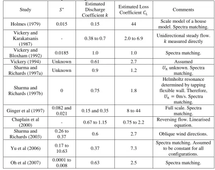
(17) building at Texas Tech University. Pearce and Sykes (1999) tested a series of flexible roof structures in the wind tunnel and also concluded that using an effective volume was satisfactory in describing the internal pressure response of buildings with a flexible envelope. In buildings without large openings, the external pressure affects the internal pressure by enabling air flow in and out of the building through the porosity in its envelope. The amount of porosity in a building can vary extensively based on the building’s function and location. For example, a shed has higher envelope porosity than a high rise building, and tropical houses will allow greater natural ventilation than houses in temperate climates. Vickery (1986) and Vickery and Bloxham (1992) showed that the inertia of the air flow through background porosity can be ignored because it is orders of magnitude smaller than the damping caused by air flowing through porous openings. They also showed that instead of treating each porous opening independently, it was acceptable to represent the sum of the porous areas by a single effective lumped porous area. The background porosity can attenuate internal pressure in a building with a dominant opening. Vickery and Bloxham (1992) showed that internal pressure fluctuations are attenuated when the background porosity area exceeds 10% of the dominant opening area. As the background porosity increases to 30% of the dominant opening area, the mean internal pressure will be significantly reduced. Woods and Blackmore (1995) and Yu et al (2008) also studied internal pressures in buildings using a lumped background porosity term and varying dominant opening areas and found that as the ratio of the porous area to dominant opening area increases, the mean internal pressure is reduced. Guha et al (2009) developed a numerical model incorporating the background porosity into the governing equation to numerically estimate the effects of porosity on internal pressure. The governing equation with background porosity was linearised by Guha et al (2011a). The study found that a lumped leeward opening was a reasonable assumption for buildings with backgrounds porosities up to nominally 10%. Guha et al (2011b) have also performed full scale. 6.

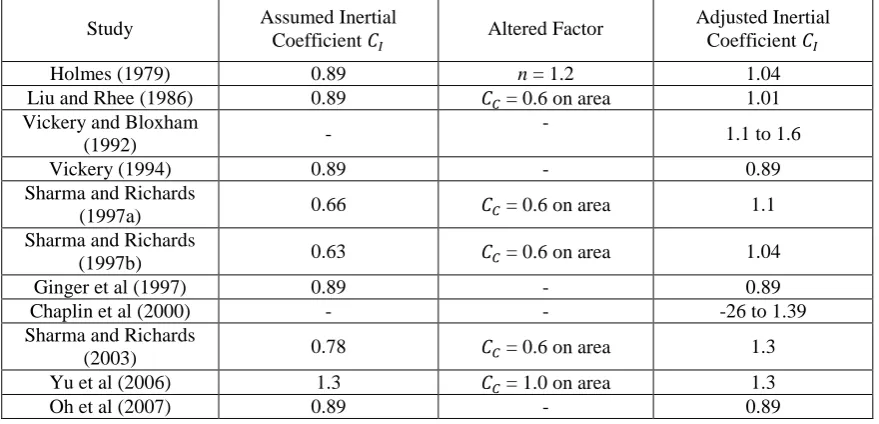
(18) monitoring on a shed and found the Helmholtz peak to be damped due to the high levels of porosity in the structure. Oh et al (2004) developed a numerical model that treated each porous opening individually, using the power law equation, suggested by Shaw (1981). The power law assumes that the flow through porous openings is similar to laminar flow in a pipe.. 2.1 Discharge Coefficient The discharge coefficient for airflow through building envelopes has been studied extensively. However, detailed studies on the discharge coefficient for flow in and out of a dominant opening have been limited in their scope. For a steady flow through a sharp edged opening, connecting two infinitely large volumes, the discharge coefficient,. is equal to 0.61 (Rouse, 1961). The discharge coefficient. can also be represented as a loss coefficient. , where. . Vickery (1991) has stated. that it is unlikely that that steady flow discharge coefficients would be applicable for the dominant opening scenario, where highly turbulent wind pressure causes air flow to move in and out of a building. Many building ventilation studies have analysed the discharge coefficients by considering the effects of parameters such as the opening area geometry, opening depth, building porosity, approaching wind direction, turbulence intensity and Reynolds number. Karava et al (2005) published a review paper summarising the effects of these parameters, which showed a large variation of the discharge coefficients between studies. They concluded that it was not possible to establish a generalized discharge coefficient and recommended that a unique discharge coefficient be selected for a given configuration. Vickery and Karakatsanis (1987) estimated the discharge coefficient for unidirectional steady flow with low turbulence by measuring the flow through a range of opening configurations in a building model using a wind tunnel. They found that for Reynolds numbers. 7.

(19) greater than about 3000, the discharge coefficient is nominally constant at 0.7. For Reynolds numbers less than 3000, the discharge coefficient ranges from 0.37 to 0.7. The Reynolds number was defined as. , where. is the kinematic viscosity of air and. is the. mean velocity at the opening. As shown in the governing Equation 2-1, air flow through a dominant opening and the internal pressure fluctuations are affected by the discharge coefficient, . Many studies apply when analysing the pressure inside a building with a dominant opening. Values for can be obtained by matching numerical simulations using Equation 2-1 with experimental results. Holmes (1979) obtained a. value of 0.15 for a dominant opening in a wind tunnel. model by comparing wind tunnel results with a numerical simulation. The lower discharge coefficient was attributed to the unsteady highly fluctuating and the reversing flow of the wind through the dominant opening caused by Helmholtz resonance. Ginger (2000) estimated the discharge coefficient for a full scale porous and flexible structure in turbulent flow to be 0.15 for a 5% opening area and 0.35 for a 2% opening area. Using similar methods of spectra matching, Yu et al. (2006) and Oh et al. (2007) estimated the discharge coefficient to be 0.37 and 0.63 respectively. An alternative method of defining the discharge coefficient was presented by Sharma and Richards (1997b), which applies a contraction coefficient inertial term and an independent loss coefficient case,. , to the opening area. , in the. in the damping term of Equation 2-1. In this. includes all losses in the system and is defined as an effective loss coefficient with a. value of 1.2 for the configurations tested by Sharma (2010). The. was empirically identified. using computational fluid dynamics when a contraction was qualitatively observed at the orifice. While the actual magnitude of the contraction on the area was not physically measured, a value of 0.6 was heuristically matched using wind tunnel experiments and numerical simulations.. 8.

(20) Few studies have examined the reversing flow condition and its effect on the discharge coefficient. Etheridge (2000) and Costola and Etheridge (2008) have studied the effects of changing flow direction on discharge coefficients for chimney stacks. However, the forward and reversing directions were considered independently and essentially treated as unidirectional. A study by Chaplin et al (2000) applied a sinusoidal reversing flow to a volume. The discharge coefficient was calculated explicitly by linearising the governing equation. The results showed that the mean discharge coefficients generally matched the steady flow theory for large openings but did not match for smaller openings. Oh et al. (2007) and Holmes and Ginger (2012) have both presented useful summaries of discharge coefficients assumed or derived in various studies. The summary showed that. has. been estimated to be in the range of 0.15 to 1.0. In the majority of studies, the discharge coefficient is determined by matching of the measured internal pressure spectrum with the spectrum of internal pressure obtained from numerical models of Equation 2-1. Table 2-1 shows a summary of discharge coefficients and loss coefficients estimated by various researchers with (if known).. 9.

(21) Table 2-1: Summary of discharge coefficients and loss coefficient from various studies Estimated Estimated Loss Discharge Study Comments Coefficient Coefficient Scale model of a house Holmes (1979) 0.015 0.15 44 model. Spectra matching. Vickery and Unidirectional steady flow. Karakatsanis 0.38 to 0.7 2.0 to 6.9 measured directly (1987) Vickery and 0.0185 1.0 1.0 Spectra matching. Bloxham (1992) Vickery (1994) Unknown 0.61 2.7 Assumed Sharma and unknown. Spectra Unknown 0.9 1.2 Richards (1997a) matching. Helmholtz resonance determined by tapping Sharma and flexible wall. Therefore, 0 0.75 1.8 Richards (1997b) m/s. Spectra matching. 0.082 and Full scale. Spectra Ginger et al (1997) 0.15 and 0.35 8 to 44 0.021 matching. Chaplain et al Reversing flow. Linearised 0.67 to 1.15 0.75 to 2.2 (2000) equation. Sharma and 0.26 to 0.6 2.7 Oblique wind directions. Richards (2003) 0.37 Spectra matching. Assumed 0.17 to Yu et al (2006) 0.37 7.3 to be constant for all 10.63 configurations. 0.0001 to Oh et al (2007) 0.63 2.5 Spectra matching. 0.008. 2.2 Inertial Coefficient The effective length,. is the estimated length of an air “slug” oscillating in and out of. an opening of a Helmholtz resonator and is given by. for very thin opening. thicknesses. Few studies have assessed the inertial coefficient,. for internal pressure. applications. Most studies have typically assumed the inertial coefficient to be a constant of 0.89, taken from Helmholtz resonator theory (Rayleigh, 1945). However, Vickery (1986) has stated that the inertial coefficient can vary from 0.89 to 2.0. The inertial coefficient can be estimated by matching the Helmholtz frequencies between experimental and numerical simulations of Equation 2-1. Several researchers have adjusted other parameters in Equation 2-1 to match Helmholtz frequencies while keeping the inertial coefficient constant. For example, Holmes (1979) adjusted the polytropic exponent,. 10.

(22) from 1.4 to 1.2, Liu and Rhee (1986) and Sharma and Richards (1997b) used a contraction coefficient in the inertial term to match the Helmholtz frequency with measured values. Vickery (1991) stated that the flow conditions for Helmholtz resonator theory are not applicable for internal pressure applications and therefore the assumed constant value for the inertial coefficient is not valid and should be adjusted. Table 2-2 presents inertial coefficients determined in various studies that indicate the parameters that were varied (if any) and presents the “effective” inertial coefficient used in Equation 2-1 to match the measured values.. Table 2-2: Summary of estimated inertial coefficients and where applicable, adjusted inertial coefficients Study. Assumed Inertial Coefficient. Holmes (1979) Liu and Rhee (1986) Vickery and Bloxham (1992) Vickery (1994) Sharma and Richards (1997a) Sharma and Richards (1997b) Ginger et al (1997) Chaplin et al (2000) Sharma and Richards (2003) Yu et al (2006) Oh et al (2007). Altered Factor. 0.89 0.89. n = 1.2 = 0.6 on area -. 0.89. -. Adjusted Inertial Coefficient 1.04 1.01 1.1 to 1.6 0.89. 0.66. = 0.6 on area. 1.1. 0.63. = 0.6 on area. 1.04. 0.89 -. -. 0.89 -26 to 1.39. 0.78. = 0.6 on area. 1.3. 1.3 0.89. = 1.0 on area -. 1.3 0.89. 2.3 Chapter Summary A building with a dominant opening can be represented as a Helmholtz resonator, where the external pressure fluctuations act as the forcing function. The Helmholtz resonator phenomenon contributes significantly to the internal pressure fluctuations in a building. The internal pressure fluctuations can be represented with respect to the opening area size and internal volume size relationship,. . A comprehensive study of the effects of a range of. on. internal pressure fluctuations are performed in this project. Internal pressure characteristics are attenuated by increasing levels of background building porosity. The background porosity can be represented as the sum of the porous openings as a single lumped porous opening in the analysis. 11.

(23) Studies on the discharge and inertial coefficients for internal pressures in buildings are limited. Previous studies show that a wide range of discharge coefficients (between 0.15 and 1.15) and inertial coefficients (between 0.89 and 1.6) have been estimated. Further research into discharge and inertial coefficients is required to explain the large range in these values.. 12.

(24) 3 Theory The unsteady, incompressible flow through an opening can be described using the unsteady discharge equation shown in Equation 3-1 (Vickery, 1986). The area averaged velocity,. is related to the flow through the opening,. and the acceleration of the flow is opening,. and opening area,. by. . The flow is driven by the pressure difference across the. . The loss coefficient and the inertial coefficient are. and. respectively.. Equation 3-1. Applying principles of mass conservation, where the flow into a building equals the flow out of the building, Liu (1975) showed that the mean internal pressure in a building is dependent on the pressure acting on the windward and leeward openings, and the sizes and discharge characteristics of the corresponding openings. The mean internal pressure is represented by Equation 3-2 in terms of pressure coefficients, Here,. is the density of air and. where. .. is the mean wind speed at roof height, . Windward and. leeward opening areas and pressures are denoted by the subscript. and , respectively. From. Equation 3-2, it can be shown that for a building with a single windward dominant opening (i.e. ) that the mean internal pressure is equal to the mean windward external pressure.. Equation 3-2. Assuming the cavity of a building with a single dominant opening behaves as a Helmholtz resonator (Holmes, 1979), the internal pressure fluctuations can be expressed by Equation 3-3. Here, the first term describes the inertia of a “slug” of air by its effective length, and the speed of sound can be expressed as pressure and. , where. is the atmospheric. is the polytropic exponent. The undamped Helmholtz frequency , where. is the effective internal volume.. 13. , is.

(25) Equation 3-3. 3.1 Building Porosity The pressure drop through porous openings in a building can also be represented by Equation 3-1. Ignoring inertial effects and assuming a lumped porous opening, the turbulent flow through porous openings can be represented by a single discharge equation in Equation 3-4.. Equation 3-4. Here. is the mean external pressure acting on the porous surfaces,. averaged velocity through the lumped porous opening and and can be related to an effective discharge coefficient. is the effective loss coefficient. , by. equation of internal pressure with a windward dominant opening opening,. is the area. . The governing , including a lumped porous. is given in Equation 3-5. The external pressure acting on the opening is given by. its coefficient. . When a building has no porosity (i.e. when. ), Equation 3-5 reduces. to Equation 3-3. This was also shown by Yu et al (2008) and Guha et al (2011a).. Equation 3-5. 14.

(26) 3.2 Dimensional Analysis Using dimensional analysis, Holmes (1979) rearranged Equation 3-3 into five nondimensional parameters to represent the fluctuating internal pressure coefficient. (Equation. 3-6). Equation 3-6. The five non-dimensional parameters are:. Here μ is viscosity of air and. is the integral length scale of turbulence. By including. a dimensionless time parameter. , Equation 3-3 can be expressed in non-. dimensional format (Equation 3-7).. Equation 3-7. The. parameters in the first and second terms of Equation 3-7 can be replaced by. the non-dimensional parameter. , where. as shown by Ginger. et al (2008). Equation 3-8 shows the governing equation in non-dimensional. format. This. implies that internal pressure fluctuations depend on the size of the opening area with respect to the size of the internal volume, and that there is a unique solution for if. and. for a given. and. ,. are known.. Equation 3-8. A building with a dominant opening and background porosity can be represented in a non-dimensional format by the addition of a sixth non-dimensional parameter. .. Equation 3-2 and Equation 3-5 can be represented in non-dimensional format shown in Equation 3-9 and Equation 3-10 respectively. Equation 3-10 is the governing equation that is. 15.

(27) used for this study. It can be shown that when. (i.e. no background porous openings), the. governing equation is equivalent to Equation 3-8.. Equation 3-9. Equation 3-10. 3.3 Discharge Coefficient The unsteady flow,. through an opening,. , driven by a pressure difference. , was. described by the discharge equation given in Equation 3-1. For the purpose of this study, the discharge coefficient is considered as a time averaged “mean” value. The discharge coefficient for an opening is a function of the velocity coefficient,. and contraction coefficient,. :. Equation 3-11. where,. Equation 3-12. Equation 3-13. Under steady flow, the vena contracta is the point where the streamlines first become parallel and where the air jet has the smallest area represented in Figure 3-1 at A-A. For steady. 16.

(28) flow through a two-dimensional, sharp edged circular orifice connecting two infinitely large volumes, steady flow theory gives. and. 0.99 or 1 (Rouse, 1959).. This gives a discharge coefficient of 0.6 to 0.61.. Figure 3-1: Location of the vena contracta for a freely flowing fluid. 3.4 Inertial Coefficient The mass of a “slug” of air can be defined by the density and volume of the air “slug”. From Helmholtz resonator theory, the volume of the “slug” can be estimated by the cross sectional area of the orifice and an effective length. The effective length. , is the length of the. air “slug” oscillating at an opening and can be expressed as Equation 3-14. Equation 3-14. Here,. is the length of the opening and. is the extended length of the air “slug”. beyond the opening. However, when opening lengths are small (i.e. windows and doors),. can. be ignored. The extended length represents the oscillating air just outside the opening. Figure 3-2 shows a schematic of a “slug” of air oscillating in a windward dominant opening.. 17.

(29) Figure 3-2: Effective length of an air “slug” oscillating at the opening of a building. Rayleigh (1896) estimated the upper and lower bound extended lengths for circular openings in Helmholtz resonators to be. and. , where is the radius of. opening. In practice, dominant openings are typically rectangular. Malecki (1969) provides estimates of and. for rectangular openings to be. , where. is the breadth of the opening. is a coefficient based on the ratio of the length to breadth. Holmes (1979) and Vickery. (1986) found that the best match for internal pressure wind tunnel studies was an extended length using an approximately circular shape given by. , where. . When the volume of air is oscillating in a volume with two open ends, such as a tube, the air on both ends of the opening are incorporated multiplying. 18. by two..

(30) 4 Wind Tunnel Methodology and Results 4.1 Experimental Setup A series of scale model wind tunnel tests were performed for this study. The dominant opening external pressure obtained from wind tunnel results were used for numerical simulations. All experiments described herein were performed at the wind tunnel building at the School of Engineering and Physical Sciences, in James Cook University.. 4.2 Wind Tunnel Specifications Wind tunnel measurements were carried out in the atmospheric boundary layer wind tunnel at James Cook University with dimensions 2.0m height, 2.5m width and 22.0m length. The atmospheric boundary layer flow was modelled at 1/200 for Terrain Category 2, as defined by AS/NZS 1170.2 (2011). The atmospheric boundary layer was modelled by installing a 250mm trip board at the inlet, immediately followed by a fetch of carpet to simulate terrain roughness. Tests were conducted at a mean reference wind speed of approximately 10 m/s at roof height,. (height = 100mm model scale). The mean velocity profile and turbulence. intensity profile of the simulated boundary layer flow and the boundary layer profile as defined by Deaves and Harris (1978) are shown in Figure 4-1. The velocity spectrum of the wind speed at roof height is shown in Figure 4-2 and the integral length scale of turbulence height was estimated to be 300mm.. 19. at roof.

(31) Elevation (mm). 500 450 400 350 300 250 200 150 100 50 0 0. 0.2. 0.4. 0.6. 0.8 U/U500mm. 1. 1.2. 1.4. WT Mean Velocity. D&H Mean Velocity. WT Turbulence Intensity. D&H Turbulence Intensity. 1.6. Figure 4-1: Wind tunnel profiles for Terrain Category 2 compared to AS/NZS1170.2 profiles. Su ( f ).  u2. Frequency (Hz). Figure 4-2: Velocity spectrum of approaching wind at roof height (100mm). Pressures were measured using the Dynamic Pressure Measurement System (DPMS) from Turbulent Flow Instrumentation. The DPMS software is used to tune the tubing system transfer functions. For this study 1m length tubes with 1.5mm inner diameter were used. All pressures were filtered at 625Hz and sampled simultaneously at 1250Hz for 30 seconds. Each test configuration listed in Table 4-1 was repeated five times. The mean, standard deviation, 20.

(32) maximum and minimum pressures were obtained in each run were averaged and presented in pressure coefficient format (. ) to give. ,. ,. and. values. respectively. 4.2.1. Wind Tunnel Model A Perspex model building with the dimensions 400mm x 200mm x 100mm was. constructed for wind tunnel testing. The model was extended by 600mm below the wind tunnel floor. Solid foam blocks were inserted into the building to vary the volume by 3 (V3), 5 (V5) and 7 (V7) times the initial volume of 400mm x 200mm x 100mm. The wind tunnel model and additional volume is shown in Figure 4-3. A dominant opening was centred on one of the 400mm walls. For this study, a single wind direction where the dominant opening is on the windward wall was studied. In addition to the varying volume, a series of four dominant opening configurations with varying area were also tested. They were 20mm x 20mm (A1), 50mm x 25mm (A2), 50mm x 50mm (A3) and 50mm x 80mm (A4).. Figure 4-3: Scale model with dimensions 400mm x 200mm x 100mm with a 600mm extension below the wind tunnel floor (All dimensions presented in mm). 21.

(33) Background porosity was modelled by installing 64 x 1.5 mm diameter holes and 54 x 3 mm diameter holes uniformly on the two side walls, the leeward wall and the roof. These porous openings could be closed or opened as needed. The porosity configurations tested were no porosity (P1), only 1.5mm diameter holes open (P2), only 3mm diameter holes open (P3) and all 1.5mm and 3mm diameter holes open (P4). Figure 4-4 shows the location and spacing of the porous openings.. Roof. Side Wall. Leeward Wall. Figure 4-4: Location of 1.5mm and 3mm hole diameter, d of porosity for the wind tunnel model (All dimensions are presented in mm). Pressure taps were installed on the roof, windward, leeward and side walls to measure the external pressures. A total of 21 roof taps, 6 taps on each side wall and 12 leeward wall taps were evenly distributed on the building surfaces. The mean lumped pressure acting on porous openings,. was obtained by area averaging measured pressures on the roof, side walls and. leeward wall pressure taps and used when analysing Equation 3-2 and Equation 3-5.. 22.

(34) The windward external pressure at the dominant windward wall opening,. was. measured in two ways. In the first method, 30 taps were staggered across an 80mm x 50mm door centred on the 400mm windward wall. The pressures were area averaged for the four corresponding dominant opening areas: A1, A2, A3 and A4. This method gives the external pressure on an intact building at the location of the dominant opening. Figure 4-5 shows the location of the external pressure taps and the corresponding dominant opening areas. In the second method, external windward pressures were measured across six taps 20mm on either side of the dominant opening and recorded simultaneously with the internal pressures. Then, internal and external pressures were used to determine net pressures,. across the windward. dominant opening.. Figure 4-5: Areas A1 to A4 and locations of the external pressure taps used for area averaging (All units presented in mm). The internal pressure,. was measured for combinations of windward wall opening. areas: A1, A2, A3, A4, volumes: V1, V3, V5, V7 and background porosities: P1, P2, P3, P4. Each windward opening area, porosity and volume gives a set of. ,. and. values given in. Table 4-1. It should be noted that volume V1 was only tested for the non porous (P1) case.. 23.

(35) Table 4-1: Test configurations opening and volume sizes, Volume (mm3) (mm2) V1 = 200x400x100 1.20 V3 = 200400300. 0.46. V5 = 200400500. 0.25. V7 = 200400700. 0.17. V1 = 200x400x100. 6.65. V3 = 200400300. 2.56. V5 = 200400500. 1.38. V7 = 200400700. 0.95. V1 = 200x400x100. 18.82. V3 = 200400300. 7.24. V5 = 200400500. 3.90. V7 = 200400700. 2.69. V1 = 200x400x100. 38.08. V3 = 200400300. 14.65. V5 = 200400500. 7.90. V7 = 200400700. 5.44. A1 = 2020 = 15.0. A2 = 5025 = 8.5. A3 = 5050 = 6.0. A4 = 8050 = 4.7. 24. , leakage area (mm2) P1 = 0 P1 = 0 P2 = 113 P3 = 382 P4 = 495 P1 = 0 P2 = 113 P3 = 382 P4 = 495 P1 = 0 P2 = 113 P3 = 382 P4 = 495 P1 = 0 P1 = 0 P2 = 113 P3 = 382 P4 = 495 P1 = 0 P2 = 113 P3 = 382 P4 = 495 P1 = 0 P2 = 113 P3 = 382 P4 = 495 P1 = 0 P1 = 0 P2 = 113 P3 = 382 P4 = 495 P1 = 0 P2 = 113 P3 = 382 P4 = 495 P1 = 0 P2 = 113 P3 = 382 P4 = 495 P1 = 0 P1 = 0 P2 = 113 P3 = 382 P4 = 495 P1 = 0 P2 = 113 P3 = 382 P4 = 495 P1 = 0 P2 = 113 P3 = 382 P4 = 495. with 0 0 0.28 0.95 1.24 0 0.28 0.95 1.24 0 0.28 0.95 1.24 0 0 0.09 0.31 0.40 0 0.09 0.31 0.40 0 0.09 0.31 0.40 0 0 0.05 0.15 0.20 0 0.05 0.15 0.20 0 0.05 0.15 0.20 0 0 0.03 0.09 0.12 0 0.03 0.09 0.12 0 0.03 0.09 0.12. and.

(36) 4.2.2. Numerical Model Internal pressures were simulated and compared with measured wind tunnel results. The. internal pressures were simulated using external pressures measured from the door areas A1, A2, A3 and A4 on the windward wall of the wind tunnel model. A first order explicit finite difference scheme was used to solve the governing equation as a function of opening area, internal volume and porous area. The first and second time derivatives of the internal pressure are shown in Equation 4-1 and Equation 4-2. Each time derivative was determined at a time step , based on the two preceding time steps, where. is the time step.. Equation 4-1. Equation 4-2. 4.3 Results and Discussion This section describes results obtained from wind tunnel experiments on the building model with varying opening areas, internal volumes and levels of porosity, presented in Table 4-1. The mean, standard deviation and peak internal pressures are presented in a nondimensional format and are compared with external pressure statistics averaged over a virtual opening area. The measured external pressures were averaged over the opening area and used to simulate internal pressures using a numerical model and matched with measured internal pressure spectra. 4.3.1. Sealed Building External and internal pressure tables of the mean, standard deviation and peak pressure. coefficients for each test configuration measured from the wind tunnel experiments are given in Appendix B. The ratios of the mean internal to external pressures for varying. values are. shown in Figure 4-6. Figure 4-6 shows that the mean internal pressure matches closely with the mean external pressure at each dominant opening configuration. These results show that. 25.

(37) generally, a variation in the internal volume will not affect the mean internal pressures as predicted by Liu (1975). For smaller values of. (i.e. configurations with the smallest opening. area A1), the mean internal pressure was measured to be less than the mean external pressure. This difference is attributed to the selection of the location of the external pressure taps which may overestimate the mean pressure.. Mean Cpi/Mean Cpw. 1.2 1.0 0.8 0.6 0.4 0.2 0.0 0.1. 1. 10. 100. S* A1. A2. A3. A4. Figure 4-6: Ratio of measured mean internal to external pressure coefficient versus. The internal pressure spectra obtained from wind tunnel measurements, on the model with openings A1, A2, A3 and A4 for volumes V1, V3, V5, and V7 are shown in Figure 4-7a, b, c and d respectively. Helmholtz resonant frequencies were estimated using the undamped Helmholtz frequency equation and are summarized in Appendix A, Table 8-3. Figure 4-7a shows that for the opening and volume configuration A1 and V3, the Helmholtz resonance occurs at a frequency of approximately 40Hz. However, as the opening area increases to areas A2, A3 and A4, the Helmholtz frequency increases to approximately 44Hz, 45Hz and 50 Hz, respectively for a constant volume of V3. This trend is also observed in for volumes V1, V5 and V7. In all cases, configurations with area A1, resulted in the smallest Helmholtz resonance peaks. This is due to the smaller opening area to internal volume ratio. At higher frequencies. 26.

(38) secondary peaks are observed, however since they occur at an order of magnitude below the Helmholtz resonance, it is not expected that they will influence the internal pressure fluctuations. It is worth nothing that the undamped Helmholtz frequencies estimated in Table 8-3 differ slightly from the measured Helmholtz frequencies from the wind tunnel experiments. In this case, the measured values are assumed to be correct since the undamped Helmholtz equation ignores damping and is therefore only an approximation. For a constant opening area and varying volume, the Helmholtz frequency reduces as volume increases. For example, in Figure 4-7b, the Helmholtz resonance for the A2V1 scenario occurs at a high frequency of approximately 120Hz. As the volume is increased, the Helmholtz frequency reduces to approximately 45Hz, 40 Hz and 38Hz for volumes V3, V5 and V7 respectively.. a). A1. 27.

(39) b) A2. c). A3. 28.

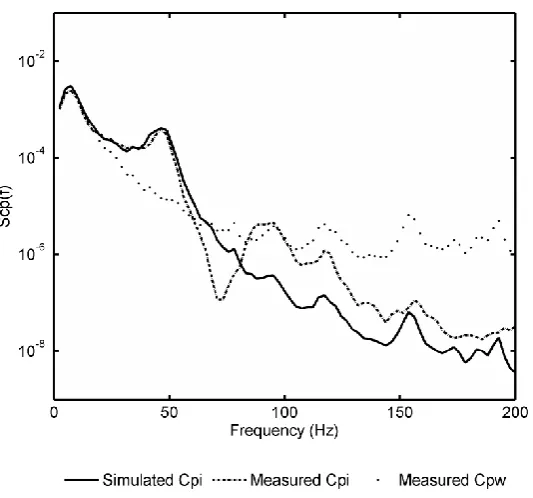
(40) d) A4 Figure 4-7: Internal pressure spectra for a) volume V1, b) volume V3, c) volume V5 and d) volume V7 with varying dominant opening areas A1 , A2, A3 and A4. The spectra shown in Figure 4-7 demonstrate the variation in internal pressure spectra with the varying sizes of opening areas and volumes. The variation in internal pressure fluctuations with respect to external pressure fluctuations is presented in Figure 4-8 as , for a range of internal volumes and opening area sizes represented by of. for a range. . The fluctuations are represented by the standard deviation and the opening area and. internal volume relationship is defined by. . The internal pressure standard deviation,. exceeds the external pressure standard deviation, about 0.4. The. is less than the. when. by about 10% when. is greater than. is less than 0.4. Figure 4-8 also compares the. ratio of measured standard deviation of internal and external pressure to the empirical formula developed by Holmes and Ginger (2012). Holmes and Ginger (2012) compare their empirical formula with those developed by Irwin (1999) and Vickery (1992). For the purpose of this study the Holmes and Ginger (2012) fit has been used. The formula is given by Equation 4-3, where A, B and C can be adjusted to fit experimental data. Holmes and Ginger (2012) suggested values of. when. . In the latter, a conservative. and. ,. and. for. is also proposed for codification. The empirical fit is 29.

(41) slightly more conservative than the measured results and appears to be suitable for design purposes.. Equation 4-3. 1.4 1.2 Cσpi/Cσpe. 1.0 0.8 0.6 0.4 0.2 0.0. 0.1. 1. 10. 100. S* ϕ5 = 15 (A1). ϕ5 = 8.5 (A2). ϕ5 = 4.7 (A4). Holmes and Ginger (2012). ϕ5 = 6 (A3). Figure 4-8: Measured ratio of internal to external pressure standard deviation versus configurations shown in brackets. The ratio of measured peak internal to external pressures versus. and. with area. for a range of. is. shown in Figure 4-9. Figure 4-9 shows similar trends as Figure 4-8, where peak internal pressures are larger than peak external pressures by up to 20%, for. greater than. approximately 0.4. Peak internal pressures are less than peak external pressures for. less than. about 0.4. Figure 4-8 and Figure 4-9 show the importance of the opening area and internal volume relationship on internal pressure fluctuations and peak. Holmes and Ginger (2012) use an empirical formula to determine ratio of the peak internal to external pressure from atmospheric turbulence, shown in Equation 4-4. Equation 4-4 is plotted in Figure 4-9 assuming a peak factor,. and turbulence intensity determined from turbulence intensity profile in. Figure 4-1,. . The empirical fit is slightly conservative when. the empirical fit is unconservative when. is greater than 1.. 30. is less than 1, however.

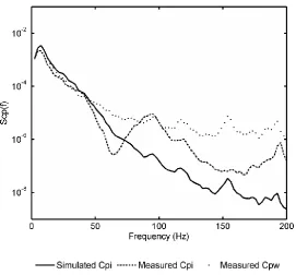
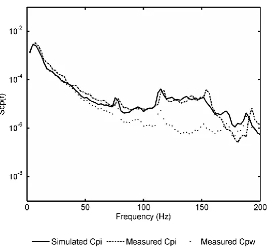
(42) Equation 4-4. Peak Cpi / Peak Cpw. 1.5. 1.0. 0.5. 0.0 0.1. 1. 10. 100. S* ϕ5 = 15 (A1) ϕ5 = 4.7 (A4). ϕ5 = 8.5 (A2) Holmes and Ginger (2012). Figure 4-9: Measured ratio of peak internal to external pressure versus shown in brackets. 4.3.2. ϕ5 = 6 (A3). and. with area configurations. Internal Pressure Simulation Figure 4-10 to Figure 4-25 show the measured external and internal pressure spectra. and the spectra obtained from numerically simulated internal pressure, for opening areas A1, A2, A3 and A4 with internal volumes V1, V3, V5 and V7. The corresponding values for the inertial coefficient,. and discharge coefficient,. used for the simulating internal pressures are. also listed in the figures. The inertial coefficient was estimated by matching the Helmholtz frequency from the numerically simulated internal pressure spectra with the measured Helmholtz frequency from the wind tunnel experiments. The discharge coefficient was estimated by matching the magnitude of the spectra from the numerically simulated internal pressure (especially near the Helmholtz resonance) with measured magnitude of the internal pressure spectra. At large frequencies secondary peaks were observed. While this study does not address this phenomenon, the peaks are 1 to 2 orders of magnitude less than the Helmholtz resonant peaks and will have a negligible effect on the internal pressure fluctuations.. 31.

(43) Figure 4-10: Measured external and internal and simulated internal pressure spectra for opening area A1 and volume V1 using = 0.3 and = 0.89 for simulations. Figure 4-11: Measured external and internal and simulated internal pressure spectra for opening area A1 and volume V3 using = 0.2 and = 1.7 for simulations. 32.


(45) Figure 4-14: Measured external and internal and simulated internal pressure spectra for opening area A2 and volume V1 using = 0.11 and =1.0 for simulations. Figure 4-15: Measured external and internal and simulated internal pressure spectra for opening area A2 and volume V3 using = 0.15 and =2.2 for simulations. 34.





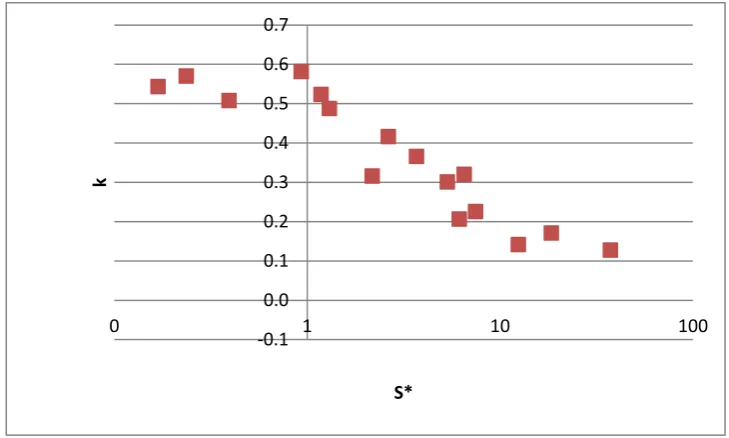
(50) Figure 4-24: Measured external and internal and simulated internal pressure spectra for opening area A4 and volume V5 using = 0.1 and = 2.1 for simulations. Figure 4-25: Measured external and internal and simulated internal pressure spectra for opening area A4 and volume V7 using = 0.15 and = 1.6 for simulations. Figure 4-10 to Figure 4-25 showed that the magnitude of. varied depending on the size. of the opening area and the size of internal volume. The estimated discharge,. 39. coefficient.

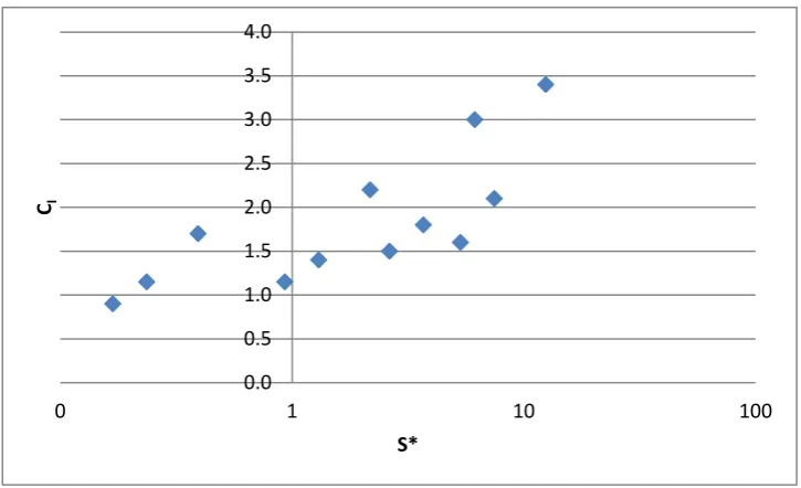
(51) ranged between 0.05 and 0.4. This range of. was less than the theoretical value used in steady. flow of 0.61. Figure 4-26 shows the variation of magnitude of. reduces with increasing. with. . The figure indicates that the. . The reduction is due to the flow at the dominant. opening being resisted by the air inside the volume. Figure 4-26 also shows that larger with decreasing. . The larger. becomes. is attributed to the flow through the opening being. similar to the flow through an orifice connecting two large volumes.. 0.6 0.5 0.4 k. 0.3 0.2 0.1 6E-16 0.1. -0.1 1. 10. 100. S* Figure 4-26: Discharge coefficient , versus. , estimated from numerical simulations. Figure 4-27 presents the inertial coefficient. obtained from matching the. internal pressure simulations with the measured value, versus. . The. from the. ranged between 0.9. and 3.4 depending on the size of opening area and size of internal volume. Figure 4-27 shows that for small values of. , the inertial coefficient is small. However, as. increases, the inertial. coefficient will also increase. These values are generally higher than the assumed inertial coefficient of 0.89 from Helmholtz resonator theory. Vickery (1994) also stated that. could be. up to a value of 2 for highly fluctuating flow. Sharma and Richards (1997b) use a separate flow coefficient to account for the contraction of the air slug at the opening that gives an overall equivalent. of approximately 1.5.. 40.

(52) 4.0 3.5 3.0. CI. 2.5 2.0 1.5 1.0 0.5 0.0 0. 1. 10. 100. S*. Figure 4-27: Inertial coefficient. 4.3.3. versus. , estimated from numerical simulations. Linearization of the Governing Equation Linearization can be used to simplify the governing equation (Equation 3-3). This. allows internal pressure fluctuations to be determined explicitly. Vickery and Bloxham (1992) and Chaplin et al (2010) have linearized the governing equation for internal pressures. Yu et al (2006) determined that the Vickery and Bloxham linearization method matched closer to the admittance obtained by numerical methods. Using the Vickery and Bloxham (1992) method of linearization, the second order term can be represented in Equation 4-5. Here,. is the. Helmholtz frequency in radians.. Equation 4-5. The damping coefficient represented by. , can then be expressed in terms of. ,. shown in Equation 4-6.. Equation 4-6. The admittance function,. for the internal pressure response with respect to the. external pressure forcing function is Equation 4-7.. 41.

(53) Equation 4-7. As the frequency approaches the Helmholtz frequency (i.e.. ) in Equation 4-7,. . Rearranging Equation 4-7 and solving for , leads to Equation 4-8. This allows the discharge coefficient to be solved explicitly, using the measured admittance function of the internal and external pressure and estimated. values from the numerical simulation.. Equation 4-8. Figure 4-28 shows the discharge coefficients estimated by using Vickery and Bloxham’s linearised equation versus. . The results shows similar trends to Figure 4-27, where. the discharge coefficient is large at smaller. values and. is small for larger. . In general, the. values for , solved using linearization are slightly larger than the discharge coefficient values estimated using the numerical simulations. However, it is worth noting that in both cases, the values estimated are less than the steady flow discharge coefficient of 0.61.. 0.7 0.6 0.5. k. 0.4 0.3 0.2 0.1 0.0 0. -0.1. 1. 10. 100. S*. Figure 4-28: Discharge coefficient , versus , estimated by linearizing the governing equation using Vickery and Bloxham method. 42.

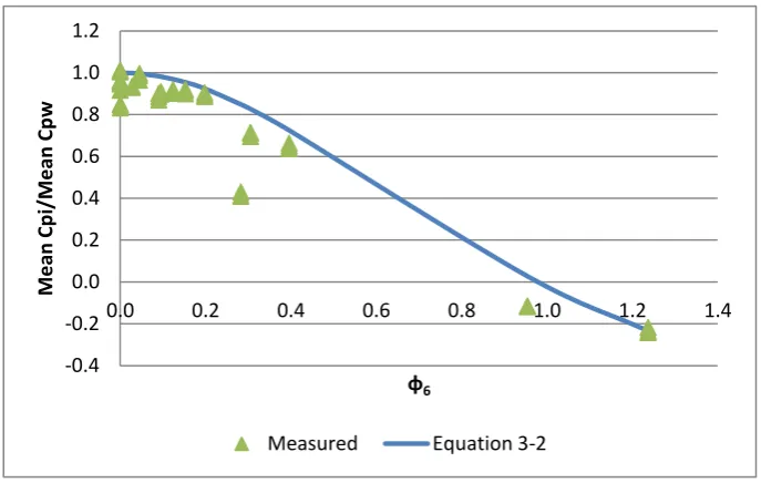
(54) 4.3.4. Porous Building Figure 4-29 compares the measured. to. ratios with theoretical values from. Equation 3-9 for varying porosity levels, and. , where. is the dominant windward opening. When. is the lumped leeward opening. (i.e. no porosity case). Using the measured mean leeward surface pressure coefficient, results show that when However, when. is less than approximately 0.2,. .. = -0.6, the theoretical. is within 10% of the. .. is larger than 0.2, the mean internal pressures are significantly reduced in. comparison with the external pressures at the windward opening. These trends are similar to those obtained by Vickery (1994).. 1.2. Mean Cpi/Mean Cpw. 1.0 0.8 0.6 0.4 0.2 0.0 -0.2. 0.0. 0.2. 0.4. -0.4. 0.6. 0.8. 1.0. 1.2. 1.4. φ6 Measured. Equation 3-2. Figure 4-29: Ratio of internal and external mean pressure coefficients to. The measured external and internal pressure spectra. with varying background. porosities P1, P2, P3 and P4, with volumes V3, V5 and V7 for opening areas A1, A2, A3 and A4 are shown in Figure 4-30, Figure 4-31, Figure 4-32 and Figure 4-33 respectively. In Figure 4-30, the background component of the internal pressure spectra for the sealed building case (P1) closely match the background component of the external pressure spectra at low frequencies. However, as porosity is introduced, the internal pressure spectra becomes. 43.

(55) dominated by the porosity and the background component of the internal pressure spectra becomes an order of magnitude less than the external pressure spectra at the opening. Figure 4-31a shows a distinct Helmholtz resonant peak at approximately 45 Hz when the building is sealed (P1). Increasing the porosity from P2, P3 to P4 progressively reduces the magnitude of the Helmholtz peak. The damping is caused by large values of. . For this case. was equal to 0.09, 0.31 and 0.40 for porosities P2, P3 and P4 respectively. When. is equal. to 0.31 and 0.40, the Helmholtz resonance is almost completely damped. Similar trends are observed in Figure 4-32 and Figure 4-33; however there is less attenuation of the Helmholtz peaks because of the smaller. values (ie. less porosity). The. values were 0.05, 0.15 and. 0.20 for Figure 4-32 and 0.03, 0.10 and 0.12 for Figure 4-33 for porosities P2, P3 and P4 respectively.. a) Opening area A1 and volume V3. 44.

(56) b) Opening area A1 and volume V5. c) Opening area A1 and volume V7 Figure 4-30: Measured external and internal pressure spectra for varying values of 0 (P1), 0.28 (P2), 0.95 (P3) and 1.24 (P4) for area A1 and volumes V3, V5 and V7. 45.

(57) a) Opening area A2 and volume V3. b) Opening area A2 and volume V5. 46.

(58) c) Opening area A2 and volume V7 Figure 4-31: Measured external and internal pressure spectra for varying values of 0 (P1), 0.09 (P2), 0.31 (P3) and 0.40 (P4) for area A2 and volumes V3, V5 and V7. a) Opening area A3 and volume V3. 47.

(59) b) Opening area A3 and volume V5. c) Opening area A3 and volume V7. Figure 4-32: Measured external and internal pressure spectra for varying values of 0 (P1), 0.05 (P2), 0.15 (P3) and 0.20 (P4) for area A3 and volumes V3, V5 and V7. 48.

(60) a) Opening area A4 and volume V3. b) Opening area A4 and volume V5. 49.

(61) c) Opening area A4 and volume V7 Figure 4-33: Measured external and internal pressure spectra for varying values of 0 (P1), 0.03 (P2), 0.10 (P3) and 0.12 (P4) for area A4 and volumes V3, V5 and V7. The ratio of the measured shown in Figure 4-34. When. to. are compared with. for ranges of. , as. is less than 0.1, the internal pressure fluctuations were greater. than the external pressure fluctuations for. values larger than 0.4. For cases when. is less. than 0.4, the internal pressure fluctuations are greatly reduced compared to external pressure fluctuations. This figure also shows that when the background porosity is increased the internal pressure fluctuations are attenuated. The magnitude of the reduction is dependent on the magnitude of the porous area to dominant opening area. in addition to. . For low. values. between 0.1 and 0.2, the attenuation of the internal pressure fluctuation is small. However when is greater than 0.2 the internal pressure fluctuations decrease by greater than 20%, especially when. is less than 0.4. For comparison, results from Vickery and Bloxham (1992) were also. plotted on Figure 4-33. The results are similar for the range of The ratio of the measured. to. values tested in this study.. is shown in Figure 4-35. The measured peak pressures. follow similar trends to the measured standard deviations. This is expected since smaller internal pressure fluctuations results in smaller peak pressures.. 50.

(62) 1.2 Cσpi /Cσpw. 1.0 0.8 0.6 0.4 0.2 0.0 0.1. 1. 10. 100. S* φ6 < 0.1 0.2 ≤ φ6 < 0.4 Vickery & Bloxham (1992) φ6 < 0.1 Vickery & Bloxham (1992) 0.2 ≤ φ6 < 0.4. 0.1 ≤ φ6 < 0.2 φ6 ≥ 0.4 Vickery & Bloxham (1992) 0.1 ≤ φ6 < 0.2. Figure 4-34: Ratio of internal and external pressure standard deviation to. for varying. 1.4 Peak Cpi / Peak Cpw. 1.2 1.0 0.8 0.6 0.4 0.2 0.0 0.1. 1. 10. 100. S* φ6 < 0.1. 0.1 ≤ φ6 < 0.2. 0.2 ≤ φ6 < 0.4. φ6 ≥ 0.4. Figure 4-35: Ratio of internal and external peak pressure coefficient to. 4.3.5. for varying. Internal Pressure Simulation The spectra of the internal pressure simulations using Equation 3-5 were matched with. measured internal pressure spectra obtained from the wind tunnel results by varying the parameters:. ,. and. , where. is the lumped background porosity discharge coefficient.. The windward wall opening discharge coefficient,. and inertial coefficient. obtained from. the sealed building case (P1), were assumed to be the same for the porous cases. The lumped background leakage discharge coefficient. was adjusted to match internal pressure spectra for 51.

(63) P2, P3 and P4. A comparison of the measured external pressure spectra and measured and simulated internal pressure spectra for configurations A2V7 and A4V7 with porosities of P1, P2, P3 and P4 are presented in Figure 4-36 and Figure 4-37, respectively. The figures also show the. and. used for simulations.. a) P2,. b) P3,. 52.

(64) c) P4, Figure 4-36: Area A2 and internal volume V7 for porosities with a constant. a) P2,. 53. and varying.

(65) b) P3,. c) P4, Figure 4-37: Area A4 and internal volume V7 for porosities with opening. Figure 4-38 shows the effective discharge coefficient area with increasing. and varying. . The estimated. 0.15 and varying. for the background leakage. values have a large variation ranging. from 0.05 to 0.5. Figure 4-38 shows that in general, for larger. values, the estimated. values tend to decrease. This may seem unexpected, however it is possible that in scenarios 54.

(66) which exhibit a strong Helmholtz phenomenon (ie. reversing flow at the dominant opening) could decrease the porous opening discharge coefficient, even if it is large.. 0.6 0.5. kL '. 0.4 0.3 0.2 0.1 0 0. 1. 10. 100. S* φ6 < 0.1. 0.1 ≤ φ6 < 0.2. 0.2 ≤ φ6 < 0.4. Figure 4-38: Discharge coefficient for background porosity. φ6 ≥ 0.4. with increasing. Figure 4-39 shows the variation of lumped background porosity discharge coefficient, with the dominant opening discharge coefficient, Here, it is assumed that. for varying porosity configurations.. is not influenced by an increase in the background porosity and is. taken as the values determined from the non porous building case. The results show, that when the dominant opening discharge coefficient is small, the porous opening discharge is also small. An increase in the. values results in an increase in the values of. . As increasing flow passes. through the dominant opening, there is a corresponding increase in the flow through porous openings. However, when less flow passes through the dominant opening, the air flow through the porous openings are also reduced. It is worth noting, that it is possible that. could vary. depending on the level of porosity present in a building, since porous openings will cause an increase in the flow through the dominant opening. Given the current testing configuration, it was not possible to measure the dominant opening discharge coefficient, nevertheless the general trends of the relationship between the dominant opening and porous opening discharge coefficients are valid. 55.

No results found