C
2014. The American Astronomical Society. All rights reserved. Printed in the U.S.A.
INFLUENCE OF STELLAR MULTIPLICITY ON PLANET FORMATION. II. PLANETS ARE LESS COMMON IN
MULTIPLE-STAR SYSTEMS WITH SEPARATIONS SMALLER THAN 1500 AU
Ji Wang1, Debra A. Fischer1, Ji-Wei Xie2, and David R. Ciardi3
1Department of Astronomy, Yale University, New Haven, CT 06511, USA;[email protected] 2Department of Astronomy & Key Laboratory of Modern Astronomy and Astrophysics
in Ministry of Education, Nanjing University, Nanjing 210093, China
3NASA Exoplanet Science Institute, Caltech, MS 100-22, 770 South Wilson Avenue, Pasadena, CA 91125, USA Received 2014 May 15; accepted 2014 July 11; published 2014 August 4
ABSTRACT
Almost half of the stellar systems in the solar neighborhood are made up of multiple stars. In multiple-star systems, planet formation is under the dynamical influence of stellar companions, and the planet occurrence rate is expected to be different from that of single stars. There have been numerous studies on the planet occurrence rate of single star systems. However, to fully understand planet formation, the planet occurrence rate in multiple-star systems needs to be addressed. In this work, we infer the planet occurrence rate in multiple-star systems by measuring the stellar multiplicity rate for planet host stars. For a subsample of 56Keplerplanet host stars, we use adaptive optics (AO) imaging and the radial velocity (RV) technique to search for stellar companions. The combination of these two techniques results in high search completeness for stellar companions. We detect 59 visual stellar companions to 25 planet host stars with AO data. Three stellar companions are within 2 and 27 within 6. We also detect two possible stellar companions (KOI 5 and KOI 69) showing long-term RV acceleration. After correcting for a bias against planet detection in multiple-star systems due to flux contamination, we find that planet formation is suppressed in multiple-star systems with separations smaller than 1500 AU. Specifically, we find that compared to single star systems, planets in multiple-star systems occur 4.5±3.2, 2.6±1.0, and 1.7±0.5 times less frequently when a stellar companion is present at a distance of 10, 100, and 1000 AU, respectively. This conclusion applies only to circumstellar planets; the planet occurrence rate for circumbinary planets requires further investigation. Key words: methods: observational – methods: statistical – planetary systems – planets and satellites: fundamental parameters – techniques: high angular resolution – techniques: photometric
Online-only material:color figures
1. INTRODUCTION
The majority of the stars in the solar neighborhood belong to multiple-star systems (Duquennoy & Mayor1991; Fischer & Marcy1992; Raghavan et al.2010; Duchˆene & Kraus2013). In multiple-star systems, many planets have been detected. Some planets are detected in circumbinary orbits (P-type; Dvorak
1982), where the planet orbits both stars (e.g., Doyle et al.
2011; Welsh et al.2012; Schwamb et al.2013). Some others are detected in circumstellar orbits (S-type), where the planet orbits only one of the stars (e.g., Cochran et al.1997; Eggenberger et al.
2004). Compared to our statistical knowledge of planets around single stars (Cumming et al.2008; Howard et al.2010; Mayor et al.2011; Wright et al.2012; Mann et al.2012; Dressing & Charbonneau2013; Gaidos2013; Swift et al.2013; Kopparapu
2013; Petigura et al.2013; Petigura et al. 2013; Bonfils et al.
2013; Parker & Quanz2013), our understanding of planet forma-tion in multiple-star systems is rather limited; the planet occur-rence rate in multiple-star systems is still largely unconstrained. Planets in multiple-star systems can be studied by either searching for planets in known multiple-star systems, or search-ing for stellar companions in known planetary systems. There have been a few studies to search for planets in known multiple-star systems (e.g., Konacki2005; Eggenberger & Udry2007; Konacki et al.2009; Toyota et al.2009). However, this direct method is prone to flux contamination of stellar companions, which affects measurement precision (Wright et al.2012). In comparison, the technical challenges are dramatically reduced for detecting stellar companions in known planetary systems; it is easier to search for a star than it is to search for a planet.
Determination of the stellar multiplicity rate for planet host stars solves the inverse problem of measuring the planet occurrence rate in multiple-star systems (Wang et al.2014). If planet host stars are rarely in multiple-star systems, this would indicate a low planet occurrence rate in these systems.
There have been numerous studies that have measured the stellar multiplicity rate of planet host stars. Most of these studies used imaging techniques, such as the adaptive optics (AO) imaging (Luhman & Jayawardhana2002; Patience et al.
2002; Eggenberger & Udry 2007; Eggenberger et al. 2011; Adams et al. 2012, 2013; Law et al. 2013; Dressing et al.
2014), Lucky Imaging (Daemgen et al. 2009; Ginski et al.
2012; Lillo-Box et al. 2012; Bergfors et al. 2013; Lillo-Box et al.2014), speckle imaging (Horch et al.2012; Kane et al.
2014), wide field imaging (Mugrauer et al.2007; Mugrauer & Neuh¨auser2009),Hubble Space Telescopeimaging (Gilliland et al.2014), and other techniques (Raghavan et al.2006,2010; Roell et al.2012). These studies have mostly reached similar conclusions that the stellar multiplicity rate of planet host stars is lower than or comparable to that for field stars in the solar neighborhood. Among these studies, some focused on stars hosting planets detected in ground-based radial velocity (RV) or transiting surveys (Luhman & Jayawardhana2002; Patience et al. 2002; Eggenberger et al. 2004; Raghavan et al. 2006; Mugrauer et al.2007; Eggenberger & Udry2007; Daemgen et al.
The Astrophysical Journal, 791:111 (16pp), 2014 August 20 Wang et al. In comparison, the Kepler mission (Borucki et al. 2011;
Batalha et al.2013; Burke et al. 2014) did not strongly bias against multiple-star systems: (1) the low-angular-resolution KeplerInput Catalog images (Brown et al.2011) did not reveal close binaries; (2) multiple-star systems (e.g., eclipsing binaries) received continued observation after detection. Therefore, the bias of ground-based surveys is not a major concern for studies ofKeplerplanet host stars (Lillo-Box et al.2012; Adams et al.
2012; Horch et al.2012; Adams et al.2013; Law et al.2013; Dressing et al. 2014; Kane et al.2014; Gilliland et al.2014; Lillo-Box et al.2014). However, there is a detection bias against transiting planets in multiple-star systems. The transit depth is shallower due to the additional flux from stellar companions, which makes planet detection more difficult. This bias has to be taken into consideration when measuring the stellar multiplicity rate for planet host stars.
It is commonly accepted that planet formation may be disrupted in multiple-star systems with small separations (e.g., ∼10–200 AU). This is supported by both simulations (Th´ebault et al.2006; Jang-Condell2007; Quintana et al.2007; Paardekooper et al. 2008; Kley & Nelson 2008; Xie et al.
2010; Th´ebault2011) and observations (Desidera & Barbieri
2007; Bonavita & Desidera2007; Kraus et al.2012). Therefore, surveys for gravitationally bound stellar companions around planet host stars provide the best path for understanding planet formation in multiple-star systems. High-resolution imaging techniques are efficient for separations greater than 0.1, and spectroscopic measurements are efficient at detecting stellar companions at smaller separations.
To carry out this work, we select a sample of 56 stars hosting planet candidates from theKepler mission to search for potential stellar companions using the RV and the AO imaging techniques. The RV technique is sensitive to short-period stellar companions, and the AO technique is sensitive to those further out. The combination of these two techniques is sensitive to a larger range of semi-major axes, and results in a survey with much higher completeness than previous studies. We consider the detection bias against transiting planets in multiple-star systems, and correct for this when calculating the stellar multiplicity rate for planet host stars. We emphasize that we only consider planets in S-type circumstellar orbits.
The paper is organized as follows. We describe our sample and the sources for their RV and AO data in Section 2. In Section3, we present the analyses of available data: searching for stellar companions to planet host stars using the RV and AO techniques. In Section4, we introduce a method of correcting for detection bias against planets in multiple-star systems, and apply it to the measurement of stellar multiplicity rate for planet host stars. We then calculate the planet occurrence rate for single and multiple star systems by comparing their multiplicity rates. Discussion and summary are given in Section5.
2. SAMPLE DESCRIPTION AND DATA SOURCES
RV and AO data are provided by the Kepler Community Follow-up Observation Program4 (CFOP). Since RV data are
critical for probing stellar companions on close orbits, we select 56KeplerObjects of Interest (KOIs) with at least three RV data points, for which the long-term RV acceleration due to a stellar companion may be measured. The RV data were taken with the HIRES instrument (Vogt et al.1994) at the Keck I telescope, and reported in Marcy et al. (2014).
4 https://cfop.ipac.caltech.edu
The AO data for these 56 KOIs were taken at different observatories including Keck, MMT, Gemini, Lick, Palomar, and WIYN. A summary of the sample and data sources is given in Table 1. Information on KOIs is provided by the NASA Exoplanet Archive (NEA; Huber et al.2014).5 All the stars in
our sample are solar-type stars with effective temperature (Teff) in the range between 4725 K and 6300 K, and surface gravity (logg) in the range of 3.9 and 4.7. There are 27 (48% of the sample) multi-planet systems.
3. DETECTIONS AND CONSTRAINTS ON STELLAR COMPANIONS TO PLANET HOST STARS
We use three techniques to detect and constrain stellar com-panions around planet host stars: the RV technique (Section3.1), the AO imaging technique (Section 3.2), and the dynamical analysis (DA, Section3.3). These three techniques are comple-mentary and sensitive to different parts of parameter space. The RV technique is sensitive to close-in companions with small to intermediate mutual inclinations with respect to the planet orbital planes; the DA technique is sensitive to companions at large mutual inclinations; and the AO imaging technique is sensitive to stellar companions at larger separations. We will discuss in this section how we use these techniques to detect stellar companions and constrain their presence.
3.1. RV Detections and Completeness
We use the Keplerian Fitting Made Easy package (Giguere et al.2012) to analyze the RV data. The procedure are described as follows. We first calculate the root mean square (RMS1 in
Table2) of the RV data. If RMS1 is five times higher than the
median reported RV uncertainties,δv, then we mark a variability flag. For systems marked with variability flags, we first fit the RV data with a linear trend, or a long-period orbit due to a nontransiting object. The systems with a significant linear trend (3σ) or the signal of an additional nontransiting object will be marked with a slope flag or a nontransiting component flag. The linear trend or the long-period orbit is then removed.
For the RV residuals after removing the linear trend or the long-period orbit, and the RVs for systems with no variability flag, we consider two cases. First, if the system has only one detected KOI, then we fit the RV data with a circular Keplerian orbit allowing only the RV semi-amplitude to change. If the resulting RMS (RMS2) is smaller than RMS1, then RMS2 is
used in subsequent analyses; otherwise RMS1is used. Second,
if the system has multiple KOIs, then we choose the one KOI causing the largest RV variation. When deciding which planet in the KOI causes the largest RV variation, we assume the planet mass–radius relationship from Lissauer et al. (2011), and calculate the nominal RV amplitude for each planet. Then, we fit the RV data with a circular Keplerian orbit allowing only the RV semi-amplitude to change. The minimum of RMS1and
RMS2 is used in subsequent analyses. In the above process,
fitting eccentric orbit does not significantly change the RMS. In addition, including more KOIs for multi-planet systems does not always help to reduce the RMS because of large RV measurement uncertainty relative to the small RV signals of small planets.
Among 56 stars, only one shows a long-term RV slope: KOI 69 has an RV linear trend of 12.2 ±0.2 ms−1yr−1. During 4.1 yr of RV measurements, there is no sign of deviation from
5 http://exoplanetarchive.ipac.caltech.edu/
Astrophysical
Journal
,
791:111
(16pp),
2014
August
2
0
Wang
[image:3.612.63.718.128.503.2]et
Table 1
RV and AO Data for 56 KOIs
KOI RV AO
KOI KIC α δ KP Teff logg #PL Tstart Tend #RV Telescope Band
(deg) (deg) (mag) (K) (cgs) (MJD) (MJD)
00005 8554498 289.739716 44.647419 11.665 5861.00 4.190 2 54983.516 56486.440 21 Keck Palomar Br-γJ 00007 11853905 285.615326 50.135750 12.211 5858.00 4.280 1 55041.491 56134.480 22 Keck Palomar H J 00010 6922244 281.288116 42.451080 13.563 6025.00 4.110 1 54983.540 55781.534 50 Palomar J 00017 10874614 296.837250 48.239944 13.303 5826.00 4.420 1 54984.561 55043.520 10 Palomar J 00018 8191672 299.407013 44.035053 13.369 6297.00 3.990 1 54985.594 55110.314 9 Gemini Gemini Palomar R Y J 00020 11804465 286.243439 50.040379 13.438 6011.00 4.230 1 55014.412 55761.325 16 Palomar J 00022 9631995 282.629669 46.323360 13.435 5972.00 4.410 1 55014.403 55792.438 16 Palomar J 00041 6521045 291.385986 41.990269 11.197 5909.00 4.300 3 54988.511 56533.359 64 Keck Palomar Br-γJ 00069 3544595 291.418304 38.672359 9.931 5593.00 4.510 1 55042.587 56547.339 61 Keck MMT MMT Palomar Br-γJ K J 00070 6850504 287.697998 42.338718 12.498 5443.00 4.450 5 55073.386 56533.484 38 Palomar J 00072 11904151 285.679382 50.241299 10.961 5627.00 4.390 2 55073.400 56172.301 54 MMT MMT Palomar J K J 00082 10187017 281.482727 47.208031 11.492 4908.00 4.610 5 55311.579 56533.335 65 Keck MMT MMT Br-γJ K 00084 2571238 290.420807 37.851799 11.898 5541.00 4.530 1 55073.419 55723.450 20 Palomar J 00085 5866724 288.688690 41.151180 11.018 6172.00 4.360 3 55696.490 55738.516 6 MMT MMT J K 00087 10593626 289.217499 47.884460 11.664 5510.00 4.500 1 55425.386 56521.486 26 Palomar Palomar J K 00103 2444412 291.683350 37.751591 12.593 5531.00 4.440 1 55073.441 55797.539 16 Palomar J 00104 10318874 281.194733 47.497131 12.895 4786.00 4.590 1 55377.342 56525.316 30 Keck Palomar Palomar K J K 00108 4914423 288.984558 40.064529 12.287 5975.00 4.330 2 55073.469 56145.498 22 Keck Palomar K J 00111 6678383 287.604614 42.166779 12.596 5711.00 4.410 4 55372.555 56521.442 14 Palomar J 00116 8395660 300.863983 44.337551 12.882 5865.00 4.410 4 55133.397 56532.332 33 Keck MMT K K 00122 8349582 284.482452 44.398041 12.346 5714.00 4.390 1 55073.495 56151.511 33 Keck Palomar K J 00123 5094751 290.392731 40.284870 12.365 5871.00 4.150 2 55074.492 56166.345 15 Keck Palomar K J 00137 8644288 298.079437 44.746319 13.549 5385.00 4.430 3 55075.509 56146.484 20 Palomar J 00148 5735762 299.139221 40.949020 13.040 5190.00 4.490 3 55073.527 56532.436 43 Keck Palomar K J 00153 12252424 287.997894 50.944328 13.461 4725.00 4.640 2 55313.592 56524.353 29 Keck MMT Palomar Palomar Br-γK J K 00157 6541920 297.115112 41.909142 13.709 5685.00 4.380 6 55440.501 56533.434 7 Palomar Robo-AO LP600 00180 9573539 284.394287 46.249081 13.024 5680.00 4.500 1 55074.466 55083.341 6 Palomar J 00244 4349452 286.638397 39.487881 10.734 6103.00 4.070 2 55366.603 56519.408 104 Keck Palomar Palomar Br-γJ K 00245 8478994 284.059540 44.518215 9.705 5288.00 4.590 4 55312.586 56523.237 59 Gemini Gemini Keck MMT MMT Palomar R Y Br-γJ K K 00246 11295426 291.032318 49.040272 9.997 5793.00 4.281 2 55312.582 56519.420 65 Keck MMT MMT Br-γJ K 00261 5383248 297.069611 40.525131 10.297 5692.00 4.420 1 55404.530 56518.546 36 Keck MMT MMT Br-γJ K 00263 10514430 281.273804 47.774399 10.821 5820.00 4.150 1 55395.529 55788.482 6 MMT MMT Palomar Palomar J K J K 00265 12024120 297.018829 50.408981 11.994 6040.00 4.360 1 55782.522 56532.354 27 Gemini Gemini Palomar Palomar R Y J K
The
Astrophysical
Journal
,
791:111
(16pp),
2014
August
2
0
Wang
et
[image:4.612.59.720.168.451.2]al.
Table 1
(Continued)
KOI RV AO
KOI KIC α δ KP Teff logg #PL Tstart Tend #RV Telescope Band
(deg) (deg) (mag) (K) (cgs) (MJD) (MJD)
00273 3102384 287.478516 38.228840 11.457 5783.00 4.430 1 55431.309 56613.223 20 MMT MMT J K 00274 8077137 282.492218 43.980209 11.390 6090.00 4.130 2 55403.447 56474.522 8 Gemini Gemini MMT MMT R Y J K 00283 5695396 288.530823 40.942299 11.525 5687.00 4.420 2 55433.368 56524.331 30 Keck Palomar Palomar Br-γJ K 00289 10386922 282.945648 47.574905 12.747 5812.00 4.458 2 56449.401 56532.291 5 Lick J 00292 11075737 287.326630 48.673431 12.872 5780.00 4.430 1 55377.475 56166.411 21 Keck Palomar Palomar K J K 00299 2692377 285.661652 37.964500 12.899 5538.00 4.340 1 55403.512 56530.414 32 Keck K 00305 6063220 297.354004 41.300049 12.970 4782.00 4.610 1 55403.543 56531.340 36 Keck K 00321 8753657 291.848053 44.968220 12.520 5538.00 4.340 2 55378.534 56493.368 47 Keck Lick K J 00364 7296438 295.872314 42.881149 10.087 5798.00 4.240 1 55376.346 55699.442 3 WIYN i
00365 11623629 297.486908 49.623451 11.195 5451.00 4.490 2 55402.354 56532.377 24 Palomar Palomar J K 00377 3323887 285.573975 38.400902 13.803 5777.00 4.450 3 55342.448 56506.363 16 Palomar Palomar J K 00701 9002278 283.212738 45.349861 13.725 4807.00 4.690 5 56137.475 56507.530 15 Keck K 00975 3632418 287.361816 38.714016 8.224 6131.00 3.950 1 55439.438 56486.562 44 MMT MMT J K 01431 11075279 287.022278 48.681938 13.460 5649.00 4.460 1 56472.391 56532.502 6 WIYN i
01439 11027624 290.851776 48.521339 12.849 5930.00 4.090 1 55075.273 56531.312 6 Lick J 01442 11600889 286.036346 49.614510 12.521 5476.00 4.448 1 55696.518 56446.424 17 Keck Lick K J 01463 7672940 288.258636 43.376465 12.328 6020.00 4.380 1 56027.511 56530.292 3 WIYN i
01612 10963065 284.786194 48.423229 8.769 6027.00 4.220 1 55697.588 56494.420 42 Keck Lick Br-γJ 01781 11551692 287.605591 49.523258 12.231 4977.00 4.590 3 56076.566 56112.331 9 Palomar Robo-AO LP600 01925 9955598 293.679199 46.852760 9.439 5365.00 4.430 1 55999.646 56547.332 40 Keck Palomar Br-γK 02169 9006186 285.207489 45.384350 12.404 5447.00 4.420 4 56099.455 56171.456 4 Palomar Robo-AO LP600 02687 7202957 292.615112 42.764252 10.158 5803.00 3.910 2 55999.652 56531.383 22 Palomar K 02720 8176564 295.439667 44.039162 10.338 6109.00 4.410 1 56018.575 56519.389 18 Keck Palomar Br-γK
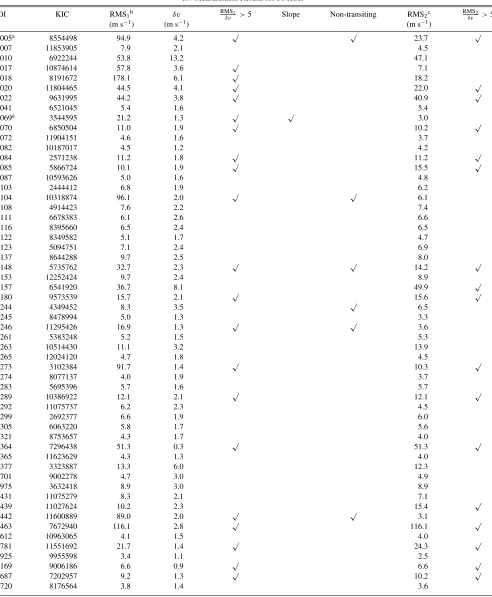
Table 2
RV Measurement Results for 56 KOIs
KOI KIC RMS1b δv RMSδv1>5 Slope Non-transiting RMS2c RMSδv2>5
(m s−1) (m s−1) (m s−1)
00005a 8554498 94.9 4.2 √ √ 23.7 √
00007 11853905 7.9 2.1 4.5
00010 6922244 53.8 13.2 47.1
00017 10874614 57.8 3.6 √ 7.1
00018 8191672 178.1 6.1 √ 18.2
00020 11804465 44.5 4.1 √ 22.0 √
00022 9631995 44.2 3.8 √ 40.9 √
00041 6521045 5.4 1.6 5.4
00069a 3544595 21.2 1.3 √ √ 3.0
00070 6850504 11.0 1.9 √ 10.2 √
00072 11904151 4.6 1.6 3.7
00082 10187017 4.5 1.2 4.2
00084 2571238 11.2 1.8 √ 11.2 √
00085 5866724 10.1 1.9 √ 15.5 √
00087 10593626 5.0 1.6 4.8
00103 2444412 6.8 1.9 6.2
00104 10318874 96.1 2.0 √ √ 6.1
00108 4914423 7.6 2.2 7.4
00111 6678383 6.1 2.6 6.6
00116 8395660 6.5 2.4 6.5
00122 8349582 5.1 1.7 4.7
00123 5094751 7.1 2.4 6.9
00137 8644288 9.7 2.5 8.0
00148 5735762 32.7 2.3 √ √ 14.2 √
00153 12252424 9.7 2.4 8.9
00157 6541920 36.7 8.1 49.9 √
00180 9573539 15.7 2.1 √ 15.6 √
00244 4349452 8.3 3.5 √ 6.5
00245 8478994 5.0 1.3 3.3
00246 11295426 16.9 1.3 √ √ 3.6
00261 5383248 5.2 1.5 5.3
00263 10514430 11.1 3.2 13.9
00265 12024120 4.7 1.8 4.5
00273 3102384 91.7 1.4 √ 10.3 √
00274 8077137 4.0 1.9 3.7
00283 5695396 5.7 1.6 5.7
00289 10386922 12.1 2.1 √ 12.1 √
00292 11075737 6.2 2.3 4.5
00299 2692377 6.6 1.9 6.0
00305 6063220 5.8 1.7 5.6
00321 8753657 4.3 1.7 4.0
00364 7296438 51.3 0.3 √ 51.3 √
00365 11623629 4.3 1.3 4.0
00377 3323887 13.3 6.0 12.3
00701 9002278 4.7 3.0 4.9
00975 3632418 8.9 3.0 8.9
01431 11075279 8.3 2.1 7.1
01439 11027624 10.2 2.3 15.4 √
01442 11600889 89.0 2.0 √ √ 3.1
01463 7672940 116.1 2.8 √ 116.1 √
01612 10963065 4.1 1.5 4.0
01781 11551692 21.7 1.4 √ 24.3 √
01925 9955598 3.4 1.1 2.5
02169 9006186 6.6 0.9 √ 6.6 √
02687 7202957 9.2 1.3 √ 10.2 √
02720 8176564 3.8 1.4 3.6
Notes.
aKOIs considered in multiple-star systems. See Sections3.2.4and3.2.5for detailed discussions. bRMS of the RV measurements.
The Astrophysical Journal, 791:111 (16pp), 2014 August 20 Wang et al.
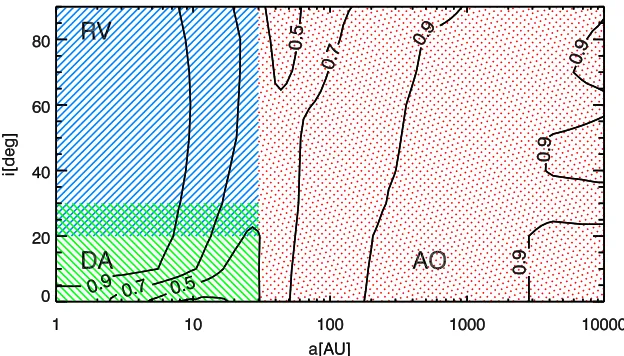
Figure 1.Median completeness contours for three techniques used to detect and constrain stellar companions to planet host stars. These three techniques are sensitive to different parts of thea−iparameter space. The radial velocity (RV) technique is sensitive to stellar companions within∼30 AU and with small or intermediate mutual inclinations to planet orbital planes (blue hatched region). The dynamical analysis (DA) technique is sensitive to a similar range of separations but larger mutual inclinations (green hatched region). The adaptive optic (AO) technique is sensitive to stellar companions at wider orbits (red dotted region). The combination of these three techniques contributes to a survey of stellar companions with high completeness.
(A color version of this figure is available in the online journal.)
the linear trend, indicating that the companion is at least 4 AU away. More discussion regarding this system will be given in Section3.2 after considering the AO data. Six systems have nontransiting objects revealed by the RV data: KOI 5, KOI 104, KOI 148, KOI 244, KOI 246, and KOI 1442. The latter five are known nontransiting planets (Marcy et al.2014). KOI 5 shows a parabolic acceleration, but the period of the nontransiting object is unconstrained. We will discuss KOI 5 more in Section3.2
with the addition of AO data. For 15 cases, RMS is still five times higher than the reported RV measurement uncertainty after considering a nontransiting object, or the KOI planet dominating the RV variability. The “excessive” RV variability may be attributed to the following factors or their combinations: very limited number of RV data points, an underestimated RV measurement uncertainty, excessive stellar activity, and additional stellar or planetary components. We find that 12 out of the 15 KOIs with “excessive” RV variation have fewer than 21 RV measurements, which is the median number of RV measurements for the 56 KOIs in our sample. Seven of them have fewer than 10 RV measurements. The limited number of RV measurements would result in an improper RV orbital fitting, which leads to a higher RMS. In addition, RV jitter is not considered in the reported RV uncertainty in Table2. After considering a typical RV jitter of 1–3 m s−1 for Kepler stars with RV measurements (Marcy et al.2014), 10 out of the 15 KOIs with “excessive” RV variation have less than five times of the RV uncertainty. KOI 22 remains the only KOI in our sample with “excessive” RV variation that cannot be explained by either the limited number of RV measurements or stellar activity.
We study the completeness of searching for stellar compan-ions by simulatcompan-ions following the subsequent procedures. We first define a parameter space,a−ispace, whereais the sepa-ration of a companion star, andiis the mutual inclination of the sky plane and the companion star orbital plane. We divide the parameter space into many fine grids (Δa=0.5 AU,Δi=10◦). For each star, we simulate 1000 companion stars on each grid, and count how many simulated companion stars are detected given the time baseline, observation epochs, and measurement uncertainties of the RV data. Specifically, we generate a syn-thetic RV data set for each of the simulated companion stars.
Observation epochs and measurement uncertainties remain the same as the original RV data. If the RMS of the synthetic RV data is three times larger than the observed RV RMS, i.e., the smaller of RMS1and RMS2, then we count the simulated
stel-lar companion as a detection. The separation and mass ratio distributions of simulated stellar companions follow the nor-mal distributions reported in Duquennoy & Mayor (1991), i.e., log10a =1.49, σlog10a = 1.54; q = m2/m1 = 0.23, σq =
0.42. We use the median orbital eccentricity for binary stars (e=0.4; Duquennoy & Mayor1991) and a random periastron distribution in simulations. The median completeness contours are shown in Figure1. RV completeness drops to below 50% as separations become larger than 30 AU.
In summary, RV observations of 56 stars reveal seven non-transiting companions, five of these are previously reported planets (Marcy et al. 2014). Orbits of the other two are unconstrained because of limited RV baselines. KOI 5 shows a parabolic RV acceleration, and KOI 69 shows a linear RV trend of 12.2±0.2 ms−1yr−1. The nature of these two companions will be discussed more in the following section.
3.2. AO Detections and Completeness
The RV variation of most of stellar companions at larger separations is difficult to measure because of the long period-icity. However, the AO imaging technique is more effective in constraining stellar companions at larger separations. We will discuss in the following part how we detect and characterize stellar companions based on AO images.
3.2.1. Contrast Curve
The contrast curve of an image provides detection thresholds for detecting faint companions around a star. The procedures of calculating the contrast curve are described as follows. We define a series of concentric annuli, centered on the star, for which we calculate the median and the standard deviation of flux for pixels within these annuli. We use the value of five times the standard deviation above the median as the 5σ detection limit. The contrast curve is the 5σ detection limit as a function of the radii of concentric annuli. The median contrast curve and the 1σ
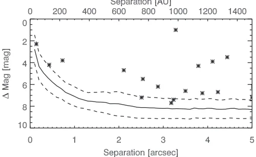
Figure 2.Median contrast curve for the AO images. Dashed lines are 1σ deviations of the contrast curve. Detections within 5are shown as asterisks. Physical projected separation in AU is calculated assuming the average distance of the sample, i.e., 300 pc. When analyzing the detection completeness, each star in our sample is treated individually for the observation band in which the AO image was taken. A total of 59 visual companions around 25 planet host stars are detected (Table3).
deviation of the AO images we use in this paper are shown in Figure2, where each pixel is converted into angular separation based on plate scale of each instrument: 0.010 pixel−1for Keck NIRC2 (Wizinowich et al. 2000), 0.011 pixel−1 for Gemini DSSI,60.019 pixel−1or 0.038 pixel−1for MMT ARIES (Sarlot
et al. 1999), 0.025 pixel−1 for Palomar PHARO (Hayward
et al.2001), 0.075 pixel−1for Lick IRCAL (Lloyd et al.2000), 0.017–0.018 pixel−1for WIYN DSSI (Horch et al.2009), and 0.043 pixel−1for Palomar Robo-AO (Law et al.2013).
3.2.2. Distance Estimation
In order to obtain the physical projected separation between detected companions and the central stars, we need to estimate the distance. The distance of a star can be measured with the distance modulus and an estimation of extinction. The extinction estimation in theVband (AV) is obtained from the
Mikulski Archive for Space Telescopes (MAST).7Details ofA V
estimation can be found in Section 6 and Section 7 in Brown et al. (2011). The distance modulus is the magnitude difference between the apparent magnitude and the absolute magnitude in theV band. The apparentV magnitude is calculated based a conversion from g and r magnitudes (Smith et al. 2002). The absoluteVmagnitude is estimated with the Yale–Yonsei (Y2) stellar evolution model (Demarque et al.2004): withTeff,
log g, age, and [Fe/H] measured from spectroscopic and/or asteroseismic observations, the absolute V magnitude can be estimated from the Y2 interpolator. For stars with an unknown AV, which is the case for seven stars, we use the distance modulus
inK band to estimate the distance with the assumption that K-band extinction is much smaller thanVband forKeplerstars. Distances for KOIs with visual stellar companion detections are provided in Table3.
3.2.3. Detection and Completeness
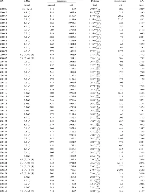
Based on the images from the CFOP, we detect a total of 59 visual stellar companions around 25 planet host stars (Table3). Fourteen stars (25%) have stellar companions within a 5radius.
6 http://www.gemini.edu/sciops/instruments/dssi-speckle-camera-north 7 https://archive.stsci.edu/
The closest companion has a projected separation of 40.9 AU (0.14) from KOI 5.
The 56 stars in our sample have an average distance of
∼300 pc. Given the contrast curve shown in Figure2, the search for stellar companions closer than∼40 AU and low-mass stars (ΔMag>8) is not complete. We therefore conduct simulations to evaluate the completeness of the AO survey. Similar to the RV completeness simulations in Section 3.1, we artificially generate 1000 companion stars at each predefined grid in the a−iparameter space. If the contrast ratio (ΔMag) between a simulation star and the central star is smaller than the value given by AO 5σ contrast curve, then we record it as a detection. Note that the contrast curves used in simulations are those calculated for each individual star in the observed band rather than the median contrast curve shown in Figure2. The AO completeness contours (median of 56 stars) are plotted in Figure1. From this plot, we show that the AO completeness is less than 50% for separations smaller than∼40 AU. At smaller separations, the RV technique becomes a much more efficient way of detecting stellar companions.
3.2.4. KOI 5
KOI 5 has a parabolic RV acceleration indicating a distant companion, but the orbit of this companion is unconstrained given only approximately four years of observation and poor phase coverage. There are many possible orbital solutions given the current RV data. Figure 3 shows two examples. If the RV acceleration is caused by the stellar companion detected by the AO imaging, then it requires a highly eccentric orbit (e = 0.92) to reasonably fit the RV data. We estimate the mass of the AO detected stellar companion to be ∼0.5 M
based on its differential magnitude in the K band (Kraus & Hillenbrand2007). Alternatively, the observed RV acceleration can be explained by a stellar companion (0.08 M) at 7 AU separation on a circular orbit. Any solutions with separations smaller than 7 AU should involve companions that fall into substellar mass regime. Therefore, we conclude that a stellar companion may exist around KOI 5, but with a separation larger than 7 AU (i.e., 0.024 angular separation).
3.2.5. KOI 69
KOI 69 shows a linear RV trend of 12.2±0.2 ms−1 yr−1, which can be caused either by a more distant star or a closer sub-stellar object. Figure4shows possible parameter space for this companion. RV data exclude any companions below the straight solid line because they are not massive enough to cause the trend. Although AO data shows nondetection for KOI 69, the AO contrast curve can put constraint on any bright stellar objects which would have been detected. After considering the constraints from AO and RV observations, if the companion causing the RV linear trend is a star, it is mostly likely to lie between 15.5 and 33.0 AU (i.e., 0.18 and 0.38 in angular separation), and its mass cannot exceed 102 Jupiter mass (2σ). If the companion mass is in the substellar regime, its mass and separation is confined to a parallelogram marked as “Substellar” in Figure4. The four vertices of the parallelogram are (5.5 AU, 10.0MJ), (9.8 AU, 10.0MJ), (27.6 AU, 80.0MJ), and (15.5 AU,
80.0MJ).
3.2.6. Visual Companions Association
The Astrophysical Journal, 791:111 (16pp), 2014 August 20 Wang et al.
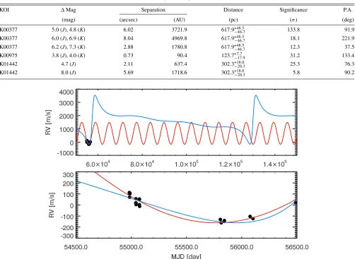
Table 3
Visual Companion Detections with AO Data
KOI ΔMag Separation Distance Significance P.A.
(mag) (arcsec) (AU) (pc) (σ) (deg)
K00005 2.3 (Br-γ) 0.14 40.9 290.9+63.2
−19.4 28.2 308.9
K00010 6.8 (J) 3.88 3663.9 944.5+100.1
−139.1 22.0 89.3
K00017 3.9 (J) 4.11 2130.7 517.9+27.6
−28.4 206.2 39.5
K00018 3.9 (J) 7.26 8241.0 1135.9+84.4
−154.0 323.2 148.2
K00018 6.3 (J) 9.68 10995.5 1135.9−+84154.4.0 32.1 344.7
K00018 6.6 (J) 3.50 3971.8 1135.9+84.4
−154.0 28.5 110.1
K00018 7.3 (J) 5.09 5783.0 1135.9−+84154.4.0 14.1 211.3
K00018 7.7 (J) 5.89 6693.3 1135.9+84.4
−154.0 9.8 106.3
K00018 7.7 (J) 10.82 12293.3 1135.9+84.4
−154.0 7.7 222.1
K00018 7.3 (J) 7.26 8241.0 1135.9−+84154.4.0 7.3 77.6
K00018 8.0 (J) 9.69 11004.0 1135.9+84.4
−154.0 6.6 339.2
K00018 8.2 (J) 7.09 8059.2 1135.9+84.4
−154.0 6.5 219.2
K00070 4.3 (J) 3.79 1058.9 279.5+25.3
−23.6 217.7 51.8
K00087 6.2 (J), 6.1 (K) 5.49 956.9 174.4+15.2
−12.1 78.2 177.2
K00087 7.4 (J), 6.6 (K) 5.53 964.1 174.4+15−12..21 28.4 75.2
K00103 7.3 (J) 9.81 2985.6 304.4−+2927..00 9.5 278.5
K00108 5.5 (J) 9.52 3357.4 352.7+36.0
−22.0 98.8 348.6
K00108 7.2 (J) 5.00 1764.4 352.7+36.0
−22.0 21.5 112.5
K00108 7.2 (J) 2.51 887.0 352.7+36.0
−22.0 19.9 74.8
K00108 7.4 (J) 3.23 1139.2 352.7+36.0
−22.0 18.2 100.9
K00108 7.4 (J) 8.90 3139.4 352.7+36.0
−22.0 17.1 19.2
K00111 7.5 (J) 7.13 2052.6 297.8+26.0
−29.1 10.8 117.7
K00111 7.8 (J) 9.07 2702.5 297.8−+2629..01 7.7 175.5
K00111 8.2 (J) 6.70 1995.1 297.8−+2629..01 8.2 96.0
K00116 3.8 (K) 8.00 2907.0 363.2+56.7
−40.3 164.1 353.5
K00116 4.8 (K) 12.96 4707.6 363.2+56.7
−40.3 51.9 144.3
K00116 6.2 (K) 7.46 2710.6 363.2−+5640..73 18.1 107.1
K00116 6.3 (K) 13.51 4907.8 363.2+56.7
−40.3 13.2 113.8
K00116 6.3 (K) 13.05 4740.8 363.2+56.7
−40.3 12.7 357.4
K00116 7.5 (K) 10.93 3969.3 363.2−+5640..73 7.5 19.7
K00116 7.3 (K) 5.79 2101.4 363.2+56.7
−40.3 6.3 141.1
K00122 6.7 (J) 4.23 1446.2 341.7+28.1
−30.3 30.0 211.3
K00123 5.2 (J) 9.52 4749.5 498.7−+2599..09 62.3 198.8
K00123 6.4 (J) 10.19 5083.7 498.7+25.0
−99.9 19.2 95.2
K00137 5.9 (J) 5.64 2471.4 438.2+37.6
−41.0 44.4 350.7
K00137 7.8 (J) 7.13 3122.2 438.2+37.6
−41.0 7.6 185.5
K00137 7.9 (J) 5.11 2240.3 438.2+37.6
−41.0 6.6 136.2
K00148 3.5 (J) 4.44 1369.1 308.7+27.0
−17.2 519.8 220.6
K00148 5.4 (J) 10.99 3391.9 308.7−+2717..02 77.0 230.1
K00148 5.5 (J) 2.54 785.2 308.7−+2717..02 69.7 245.8
K00148 6.3 (J) 8.05 2486.4 308.7−+2717..02 35.5 244
K00148 7.4 (J) 6.06 1870.7 308.7−+2717..02 13.9 238.8
K00153 6.0 (K) 8.01 1812.0 226.2+18.6
−15.1 11.2 353.4
K00153 6.9 (J), 7.6 (K) 6.17 1395.3 226.2+18.6
−15.1 4.5 298.4
K00244 2.7 (J), 2.0 (K) 8.40 2741.0 326.3+23−44..46 3231.4 287.6
K00244 7.6 (J), 7.0 (K) 8.38 2733.6 326.3+23−44..46 27.5 101.4
K00263 1.0 (J), 1.0 (K) 3.28 788.5 240.7+17.7
−38.9 2430.8 268.2
K00273 6.2 (J), 5.6 (K) 5.02 1201.8 239.6+14.7
−15.2 32.6 344.0
K00283 7.9 (K) 6.09 1266.2 208.0+21.4
−11.2 7.0 271.4
K00289 8.6 (J) 5.86 2201.2 375.9−+35569..80 5.1 88.3
K00289 7.7 (J) 3.18 1195.0 375.9+355.0
−69.8 6.1 308.6
K00292 4.2 (K) 0.43 154.9 358.5+40.9
−28.3 43.2 119.4
K00365 7.7 (J), 6.6 (K) 7.12 1129.9 158.8+15−19..17 13.3 313.7
Table 3 (Continued)
KOI ΔMag Separation Distance Significance P.A.
(mag) (arcsec) (AU) (pc) (σ) (deg)
K00377 5.0 (J), 4.8 (K) 6.02 3721.9 617.9+48.5
−46.7 133.8 91.9
K00377 6.0 (J), 6.9 (K) 8.04 4969.8 617.9+48.5
−46.7 18.1 221.9
K00377 6.2 (J), 7.3 (K) 2.88 1780.8 617.9+48−46.5.7 12.3 37.5
K00975 3.8 (J), 4.0 (K) 0.73 90.4 123.7+7−17.7.9 31.2 133.4
K01442 4.7 (J) 2.11 637.4 302.3−+1820.0.3 25.3 76.3
K01442 8.0 (J) 5.69 1718.6 302.3+18.0
[image:9.612.149.464.512.691.2]−20.3 5.8 90.2
Figure 3.Two possible scenarios for the observed RV acceleration of KOI 5. Black dots are current RV data. Blue line shows a case in which the RV acceleration is caused by the AO detected companion with a 40.9 AU projected separation (i.e., 0.14 angular separation). A highly eccentric orbit (e=0.92) is required to reasonably fit the RV data. The red line shows another case in which a 0.08Mcompanion on a circular orbit with a 7 AU separation causes the RV acceleration. More RV data with a longer baseline are required to determine the nature of the companion causing the RV acceleration of KOI 5. The top panel shows a large time range, and the bottom panel shows a zoom-in plot to a time range with RV data.
(A color version of this figure is available in the online journal.)
The Astrophysical Journal, 791:111 (16pp), 2014 August 20 Wang et al. host stars. Lillo-Box et al. (2012) estimated that∼35%–53% of
visual companions are bonded to the primary stars within 3, and this ratio decreases with increasing angular separations. Therefore, the nonnegligible fraction of visual companions we detect are in fact unassociated with primary stars, which will decrease the stellar multiplicity rate for planet host stars.
For 12 visual companions with multi-band detections (i.e., JandKband), we test if they are physically associated with their primary stars. The procedures of the test are described as follows. We calculate theJ−K colors of visual companions based on the differential magnitudes in Table3and theJ−K colors of primary stars from the NEA. From theirJ−Kcolors, we interpolate for the absoluteK-band magnitude of companion stars based on Table 5 in Kraus & Hillenbrand (2007). With the absolute K-band magnitudes and the apparent K-band magnitudes, we calculate the distances of the visual companion stars, and check whether they are consistent with the distances of the primary stars. If the color-determined distance for the companion is 1σ different from the distance of the KOI as reported in Table3, we reject the physical association between the KOI and the visual companion star. We find inconsistent distance for 6 out of 12 visual companions. The six companions include one for KOI 87 (at 5.49 separation,d =2.9±2.2 kpc), one for KOI 153 (at 6.17 separation, d = 52±44 kpc), one for KOI 244 (at 8.40 separation,d =33±20 pc), and all three for KOI 377 (d = 3.8±2.2 kpc, d = 204±163 kpc, and
d=412±330 kpc).
3.3. Dynamical Analysis
In addition to constraints from RV and AO data, more constraints of potential stellar companions can be put on multi-planet systems (Wang et al.2014). There are 27 (48% of the sample) multi-planet systems in our sample for which we can apply the dynamical analysis (DA). The DA technique makes use of the co-planarity of multi-planet systems discovered by theKeplermission (Lissauer et al.2011). A stellar companion with high mutual inclination to the planetary orbits would have perturbed the orbits and significantly reduce the co-planarity of planetary orbits, and hence the probability of multi-planet transits. Therefore, the fact that we see multiple planet transiting helps to exclude the possibility of a highly inclined stellar companion. The DA is complementary to the RV technique because it is sensitive to stellar companions with large mutual inclinations to the planetary orbits. The parameter space the DA is sensitive to is shown in Figure1.
3.4. Combining Results from Different Techniques
For the RV and AO observations, detection completeness con-tours are calculated based on simulations given the observational constraints, such as the time baseline, cadence, measurement un-certainties, and the contrast curve. For the DA technique, numer-ical integrations give the fraction of time when multiple planets can stay with small mutual inclinations (<5◦) so that multiple transiting planets can be observed (Wang et al.2014). Note that the DA technique works only for systems with multiple planets, which account for 48% of the sample. For systems with a single transiting planet, no constraint can be given by the DA tech-nique. We denotecRV,cAO, andcDAas the completenesses at a
given point in thea−iparameter space, overall completenessc is equal to 1−(1−cRV)×(1−cAO)×(1−cDA). We note that the
calculation assumes each technique is independent and uniquely sensitive to a certain portion of the parameter space. This is
generally the case since the RV technique completeness drops quickly beyond ∼30 AU, where the AO technique sensitivity is high. Similarly, the RV and DA techniques and the DA and AO techniques have little overlap in sensitivity parameter space. The overall completeness may be overestimated at the transition space, such asa =30 AU (for RV and AO) andi = 20◦(for RV and DA), because stellar companions falling into this pa-rameter space can be detected by multiple techniques and thus the techniques become correlated. We also try another way of combining results from different techniques, in which we use the maximum completeness as the overall completeness. This approach assumes multiple techniques are correlated, however, it does not significantly change the conclusions in this paper.
The completeness is then integrated over thea−iparameter space. We assume a log-normal distribution fora(Duquennoy & Mayor1991; Raghavan et al.2010), random distribution ofi for systems with only one transiting planet, and theidistribution from Hale (1994) for systems with multiple transiting planets. The treatment for multiple transiting planet systems is detailed in Wang et al. (2014), i.e., a coplanar distribution for stellar companions within 15 AU, a random i distribution for stellar companions beyond 30 AU, and a mixture i distribution at intermediate separations between 15 and 30 AU.
4. PLANET OCCURRENCE RATE AND STELLAR MULTIPLICITY RATE
4.1. Detection Bias Against Planets in Multiple-star Systems
Planets in multiple-star systems are more difficult to find using the transiting method because of flux contamination. We discuss how this bias against planet detection in multiple-star systems can be quantified. For theKeplermission, it is a necessary condition to become a planet candidate that the signal-to-noise ratio (S/N) should be higher than 7.1 (Jenkins et al.
2010a). S/N can be calculated using the following equation:
S/N= δ CDPPeff
Ntransits, (1)
whereδis the transit depth, CDPPeff is the effective combined
differential photometric precision (Jenkins et al. 2010b), a measure of photometric noise, and Ntransits is the number of
observed transits. We use a planet in a binary system as an example to calculate the transit depth:
δ= R
2 PL
R2
∗
F∗
F∗+Fc
, (2)
whereRPL is planet radius,R∗is the radius of the star that the
planet is transiting,Fdenotes flux, and subscript∗andcindicate the planet host star and the contaminating star, respectively. Two cases are considered for the above equation. First, if the planet transits the primary star, the transit depth is diluted by a factor of two at most, whenF∗andFcare identical. Second, if the planet
transits the secondary star, the transit depth dilution effect due to flux contamination can be much larger than two even after considering the increase in the transit depth from a reducingR∗
in the first term of the equation. For an example of a solar-type star and a late-type M dwarf pair, the gain of a reducingR∗can be a factor of 100 at most, but the flux ratio between the two stars can easily exceed 104in theKeplerband.
Therefore, we conduct simulations to quantify the detection bias against planets in binary star systems. For each KOI, we
choose the one planet that gives the highest S/N. We add a companion star in the system and calculate the S/N in the presence of flux contamination for two cases: planet transiting the primary star and planet transiting the secondary star. In both cases, we assume the same period and transit duration from the NEA so thatCDP PeffandNtransitsin Equation (1) are the same,
and flux contamination (see Equation (2)) is the only factor that determines whether a planet is detected in the presence of a companion star. If the S/N is higher than 7.1, then the planet can still be detected byKepler, but with a lower significance. We randomly assign a stellar companion (secondary star) to a KOI (primary star) and repeat this procedure 1000 times for both the primary and the secondary star. We record the fraction of planet detections,α, which will be used in correcting for the bias of detecting planets in multiple-star systems (Table4). The median value ofαfor 56 stars in our sample is 0.89, implying that the detection bias is not severe, but certainly not negligible. In the simulations, we use the stellar parameters from the NEA for the primary star. When generating a stellar companion in the simulations, we assume the mass ratio distribution follows the normal distribution given in Duquennoy & Mayor (1991). The radius of the secondary star is calculated using a stellar mass–radius relationship (Feiden & Chaboyer2012). Estimation of stellar flux for both primary and secondary stars are based on Table 5 in Kraus & Hillenbrand (2007). We calculatedCDPPeff
by interpolating between 3, 6, and 12 hr CDPPs based on transit duration.
4.2. Distinguishing Planets in Single and Multiple-star Systems
TheKeplermission has provided us with a large sample of planet candidates. However, we do not know whether the planet host stars are in single or multiple stellar systems. Distinguishing planets in single and multiple-star systems allows us to sepa-rately calculate the planet occurrence rate for these two types of stars, and to understand planet formation in different stellar environments (Wang et al.2014). Follow-up observations are critical in identifying additional stellar companions in planetary systems. Even in the case of nondetection, with RV, AO, and DA techniques, we can calculate the probability of a star being in a multiple-star system based on the completeness study. For example, if the overall completeness for a companion detec-tion is 80% and the stellar multiplicity rate is 46% (Raghavan et al.2010), then the probability of the star having an undetected companion (or being a multiple-star) is (100%–80%)×46%= 0.092. Following this procedure, we calculate the number of multiple-starsNMand the number of single starsNS. SinceNM
andNS are the sums of probabilities, they will not necessarily
be integers:
NM =
n
i=1
[pM(i)/α(i)], NS= n
i=1
[1−pM(i)], (3)
wherenis the total number of stars in the sample,pM(i) is the probability of theithstar being a multiple-star system,α(i) is the
correction factor for the detection bias for planets in multiple-star systems. The above equation is similar to Equation (6) in Wang et al. (2014) except for the correction factor α. Note that there is an implicit correction factor for single stars in Equation (3). However, the correction factor for single stars is one. If a stellar companion is detected for a KOI, thenpMis
assigned to one, andαis also assigned to one because no bias exists in this case since a planet has already been detected in
a multiple-star system. For an AO detected stellar companion, setting pM to one is an overestimation because the physical
association of visual stellar components is not yet established. Therefore, the stellar multiplicity rate that will be subsequently determined is an upper limit.
We then definefas the fraction of stars with planets,fcan be separated into two components:
f =(1−MR)×fS+ MR×fM, (4)
where MR is the global stellar multiplicity rate,fS andfMare
the fraction of stars with planets for single and multiple-star systems, respectively. The ratio offS andfM can be calculated
in the following equation:
fS
fM =
NS
1−MR
NM
MR
. (5)
With Equations (4) and (5),fS andfM can be solved
indepen-dently given thatNSandNMcan be measured and thatfcan be
measured globally (e.g., Fressin et al.2013). In addition, the MR for planet host stars (MRPL) can be calculated and compared to
a global MR:
MRPL=
NM
NM +NS
, (6)
4.3. Stellar Multiplicity Rate for Planet Host Stars
Figure5shows the comparison between the stellar multiplic-ity rate for field stars (dashed line Duquennoy & Mayor1991; Raghavan et al.2010) and that for planet host stars (blue and red hatched regions). The red hatched region is the 1σ uncertainty region for 56 stars with RV and AO observations, and the DA analysis. The error bar of NM is estimated based on Poisson
statistics. The square root of the closest integer toNMis used as
the error bar toNMunless the closest integer is zero, in which
case we used one for the error ofNM. The stellar multiplicity
rate for planet host stars is significantly lower than that of field stars until the separation reaches∼1500 AU. This implies that the influence of a stellar companion may be more profound than previously thought. The effective separation below which planet formation is significantly affected is extended to∼1500 AU. In comparison, the blue hatched region represents the 1σ uncer-tainty region for 23 stars with RV data and DA analysis, but no AO observations (Wang et al. 2014). Based on the blue hatched region, the significant difference of stellar multiplicity disappears after separation reaches 20.8 AU. Since Wang et al. (2014), we have incorporated AO data into our analyses and increased the sample size from 23 to 56. These improvements greatly strengthen the statistics in the comparison. Specifically, increasing the sample size reduces the statistical uncertainty; adding AO data helps constrain stellar companions beyond the reach of the RV technique.
4.4. Planet Occurrence Rate versus Binary Separation
With the stellar multiplicity rate for planet host stars, we can calculate the ratio of the planet occurrence rate for single and multiple-star systems according to Equation (5). Figure6
The Astrophysical Journal, 791:111 (16pp), 2014 August 20 Wang et al.
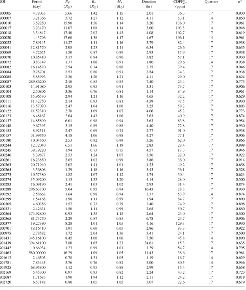
Table 4
Detection Bias of Planets in Multiple Stars
KOI Period RP R∗ M∗ Duration CDPPa
eff Quarters αb
(day) (R⊕) (R) (M) (hr) (ppm)
K00005 4.78033 5.66 1.42 1.15 2.01 36.3 17 0.930
K00007 3.21366 3.72 1.27 1.12 4.11 53.1 14 0.850
K00010 3.52250 15.90 1.56 1.14 3.20 136.0 17 0.961
K00017 3.23470 11.07 1.08 1.14 3.60 103.5 14 0.946
K00018 3.54847 17.40 2.02 1.45 4.08 102.7 17 0.619
K00020 4.43796 17.60 1.38 1.17 4.67 106.1 14 0.961
K00022 7.89145 11.27 1.11 1.16 3.79 82.4 17 0.938
K00041 12.81570 2.08 1.23 1.11 6.54 26.6 17 0.635
K00069 4.72675 1.50 0.87 0.89 2.93 17.9 17 0.938
K00070 10.85410 3.17 0.94 0.90 3.82 57.1 17 0.930
K00072 0.83749 1.37 1.00 0.91 1.80 29.6 14 0.938
K00082 16.14570 2.54 0.74 0.80 3.75 39.4 17 0.946
K00084 9.28701 2.53 0.86 0.91 3.54 34.3 17 0.938
K00085 5.85993 2.36 1.20 1.21 4.11 29.0 17 0.624
K00087 289.86200 2.10 0.85 0.83 7.40 23.4 17 0.773
K00103 14.91080 2.95 0.95 0.91 3.31 73.7 17 0.906
K00104 2.50806 3.36 0.76 0.81 1.14 84.9 17 0.961
K00108 15.96530 2.94 1.21 1.16 4.65 32.2 17 0.629
K00111 11.42750 2.14 0.93 0.81 4.59 47.5 17 0.930
K00116 13.57070 2.47 1.04 1.00 3.25 59.2 17 0.803
K00122 11.52310 2.78 1.09 1.07 4.06 45.2 17 0.773
K00123 6.48167 2.64 1.43 1.06 3.63 40.9 17 0.874
K00137 14.85890 6.01 0.98 0.94 3.63 83.8 17 0.954
K00148 9.67393 3.15 0.89 0.88 4.40 72.8 17 0.930
K00153 8.92511 2.47 0.69 0.74 2.77 91.0 17 0.938
K00157 31.99550 4.18 1.06 0.98 4.27 77.1 17 0.906
K00180 10.04560 2.53 0.92 0.99 3.26 62.0 17 0.866
K00244 12.72040 6.51 1.66 1.19 2.83 28.4 17 0.898
K00245 39.79220 1.94 0.73 0.75 4.57 17.3 17 0.946
K00246 5.39877 2.53 1.24 1.07 3.56 22.0 17 0.922
K00261 16.23850 2.65 1.02 0.99 3.86 36.0 17 0.914
K00263 20.71940 2.02 1.41 1.01 4.23 49.2 17 0.658
K00265 3.56806 1.29 1.18 1.16 3.43 36.1 17 0.528
K00273 10.57380 1.82 1.07 1.12 1.74 30.4 17 0.624
K00274 15.09200 1.13 1.55 1.20 4.14 28.0 17 0.500
K00283 16.09190 2.41 1.03 1.02 2.93 31.4 17 0.874
K00289 296.63700 5.04 0.95 0.94 16.43 28.3 17 0.930
K00292 2.58663 1.64 0.98 0.94 2.37 53.9 14 0.874
K00299 1.54168 1.98 1.11 0.99 1.94 84.7 17 0.890
K00305 4.60356 1.57 0.73 0.79 2.40 74.9 17 0.898
K00321 2.42631 1.50 1.11 0.99 2.65 50.7 17 0.850
K00364 173.92800 0.93 1.35 1.15 2.64 23.0 17 0.500
K00365 81.73750 2.29 0.87 0.85 6.78 23.7 17 0.906
K00377 19.27390 8.28 1.01 1.05 4.16 129.3 17 0.930
K00701 18.16410 1.91 0.60 0.65 2.96 83.3 17 0.922
K00975 2.78582 1.72 2.04 1.36 3.41 24.1 17 0.500
K01431 345.16100 8.45 1.00 1.06 7.50 45.8 14 0.890
K01439 394.61100 7.80 1.65 1.23 24.61 15.3 17 0.635
K01442 0.66934 1.23 0.99 1.01 1.29 54.7 14 0.795
K01463 580.00000 16.29 1.09 1.05 11.43 38.6 17 0.961
K01612 2.46503 0.78 1.31 1.05 1.19 16.7 14 0.629
K01781 7.83445 3.76 0.76 0.82 3.00 80.5 14 0.946
K01925 68.95800 1.12 0.95 0.88 2.99 15.4 17 0.658
K02169 5.45300 0.97 0.93 0.82 2.24 43.2 17 0.723
K02687 1.71683 1.90 1.94 1.12 2.11 24.2 17 0.818
K02720 6.57148 0.80 1.05 1.05 3.07 22.6 17 0.619
Notes.
aEffective combined differential photometric precision (Jenkins et al.2010b).
bCorrection factor for the bias against planet detection in binary stars. The factor ranges from zero to one, with one indicating 100% detection rate even with
the flux contamination from a companion star. See Section4.1for more details.
Figure 5.Comparison of the stellar multiplicity rate of field stars (dashed line) and planet host stars (hatched regions). The blue hatched region represents the 1σ region of the stellar multiplicity rate for 23 planet host stars with RV and DA analysis (Wang et al.2014). AO data were not incorporated, so the sensitivity of RV and DA was limited within 50 AU. For this study, AO data are used to constrain stellar companions beyond 50 AU. The red hatched region represents the 1σregion of the stellar multiplicity rate for 56 stars with RV, AO, and DA analysis. The new study shows that the stellar multiplicity rate for planet host stars is lower than that for the field stars within 1500 AU, indicating a more profound influence of stellar companions on planet formation.
(A color version of this figure is available in the online journal.)
Figure 6.Ratio of the planet occurrence rates for single and multiple-stars. Dashed line represents the value of one, a value indicating a comparable planet occurrence rate. The planet occurrence rate for single stars is much higher than that for multiple-stars within 10 AU. Beyond 10 AU, the ratios are 4.5±3.2, 2.6±1.0, and 1.7±0.5 for 10 AU, 100 AU, and 1000 AU, respectively, indicating planets in multiple-star systems are fewer than those around single stars at these separations. The planet occurrence rates become comparable between single and multiple stars when separation is larger than∼1500 AU. Error bars are calculated based on Poisson statistics and propagated through Equation (5). No error bar is shown within 10 AU because of the detection of less than one stellar companion according to Equation (3).
The deficiency of planets around multiple-stars indicates that the suppressive influence on planet formation of a stellar companion is significant at these separations. The suppressive effect decreases as separation increases, and fS and fM are
comparable at separations around∼1500 AU, indicating that stellar companions at these separations barely have any influence on planet formation. The comparison of planet occurrence rate for single and multiple-stars at other stellar separations is given in Table5.
4.5. Comparison to Previous Results
[image:13.612.44.290.310.431.2]The field of studying planets in multiple-star systems may be divided into two eras: before and after theKeplermission. Before theKeplermission, stars with giant planets are the main targets, and they are mostly detected by the RV technique. Bonavita & Desidera (2007) used a sample defined as the “uniform detectability” (UD) sample. They searched for stellar companions around stars in this sample, and found that the
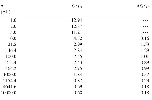
Table 5
Ratio of the Planet Occurrence Rate Between Single Stars and Multiple-Star Systems as a Function of Stellar Separation
a fs/fm δfs/fma
(AU)
1.0 12.94 · · ·
2.0 12.87 · · ·
5.0 11.21 · · ·
10.0 4.52 3.16
21.5 2.99 1.53
46.4 2.84 1.29
100.0 2.55 1.01
215.4 2.43 0.89
464.2 2.75 0.99
1000.0 1.84 0.57
2154.4 0.87 0.23
4641.6 0.69 0.18
10000.0 0.68 0.18
Notes.aError bars are calculated based on Poisson statistics and propagated
through Equation (5). No error bar is given within 10 AU because of the detection of less than one stellar companion according to Equation (3).
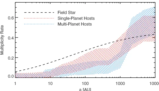
[image:13.612.317.568.339.504.2]The Astrophysical Journal, 791:111 (16pp), 2014 August 20 Wang et al.
Figure 7.Comparison of the stellar multiplicity rate for field stars (dashed line), 29 planet host stars with a single detected planet (red dotted region, 1σrange), and 27 planet host stars with multiple detected planets (blue dotted region, 1σrange).
(A color version of this figure is available in the online journal.)
has made use ofKeplerdata, and therefore mostly deals with lower-mass planets. Second, RV surveys have a much stronger bias against close-in binary stars than theKeplermission.
After theKeplersatellite was launched, studies continue on the stellar multiplicity of planet host stars. Lillo-Box et al. (2012) found that the visual companion rate for KOIs is 17.3% and 41.8% within 3 and 6, respectively. They later updated the companion rate to be 17.2% and 32.8% within 3and 6 (Lillo-Box et al. 2014). Dressing et al. (2014) found that 17.2% of KOIs have visual companions within 3. In comparison, we find that 12.5±4.7% and 48.2±9.3% of KOIs have visual companions within 3 and 6, which is consistent with their numbers. Adams et al. (2012) found that 60%, 20%, and 7% of 90 KOIs have stellar companions within 6, 2, and 0.5, respectively. We find that these numbers to be 48.2±9.3%, 5.4±3.1%, and 3.6±2.5%. In comparison, we find significantly fewer stellar companions than Adams et al. (2012) at angular separations between 0.5 and 2.0.
We therefore conduct a cross-check with their targets, and find 20 overlapping targets. For these targets, we detect 40 companions using the images from the CFOP, while they detect 33 companions. We find 17 new companions that were not reported by Adams et al. (2012). Most of the new companions are more than 6 away from central stars. We are not able to detect 10 of their companions. All of our missing detections haveΔMag larger than 7.1 mag (close to detection limit, see Figure 2), and none of them are within 2 except for KOI 18 (0.9 separation andΔmag=5.0). We suspect the difference may be a result of different thresholds for companion detections or differences in manual inspections.
We also conduct investigations on the lack of companion detections within 2.0. In the overlapping sample of 20 KOIs with Adams et al. (2012), we detect two companions within 0.5, KOI 292 (0.43), and KOI 975 (0.72). They are also detected in Adams et al. (2012), but KOI 18 with a separation of 0.9 was missed in our search. For the overlapping sample, 10.0±7.1% (2 out 20) have companions within 2. In comparison, for the rest of our sample, none of the 36 stars have companions detected within 2, which raises a concern that KOIs with close-in companions may be filtered out when conducting RV followup observations. However, it does not seem to be the case for KOI 18, KOI 292, and KOI 975, these targets receive continued
RV followup observations even after close-in companions are detected in AO images.
5. SUMMARY AND DISCUSSION
5.1. Summary
We conduct a search for stellar companions to a sample of 56 Kepler planet host stars, and compare the stellar multiplicity rate for planet host stars and the field stars in the solar neighborhood. We find that the stellar multiplicity rate for planet host stars is significantly lower than that for the field stars at stellar separations smaller than 1500 AU, indicating that planet formation is less efficient in multiple-star systems than in single stars. The influence of stellar companions plays a significant role in planet formation and evolution in multiple-star systems with separations smaller than 1500 AU.
We distinguish the planet occurrence rates for single and stars. We find that planets in S-type orbits in multiple-star systems are 4.5±3.2, 2.6±1.0, and 1.7±0.5 times less frequent than planets orbiting single stars if a stellar companion is present at distances of 10, 100, and 1000 AU, respectively. The difference in planet occurrence rate between single and multiple-star systems becomes insignificant when companion separation exceeds 1500 AU, suggesting that planet formation in widely separated binaries is similar to that around single stars. In summary, three improvements in this study allow us to better study planets in multiple-star systems. First, unlike planet host stars selected from ground-based RV and transiting surveys, our sample from theKeplermission does not have strong bias against planets in multiple-star systems. Second, we combine the RV and AO data for the 56Kepler stars, which construct a survey for stellar companions with high completeness. The DA method is also used to put further constraints on stellar companions in systems with multiple transiting planets. Third, we develop a method to quantify the detection bias of planets in multiple-star systems, which enables a fair comparison of stellar multiplicity rate.
5.2. Discussion
5.2.1. Stellar Companions to Hot Jupiter Host Stars
There are six hot Jupiter (HJ,P <10 day andRP >5R⊕) host stars in our sample. They are KOI 5, KOI 10, KOI 17,