An analysis of variation in response time of CPU scheduling algorithms as a function of load: a simulation

(1)

Rochester Institute of Technology

RIT Scholar Works

Theses

Thesis/Dissertation Collections

5-20-1986

An analysis of variation in response time of CPU

scheduling algorithms as a function of load: a

simulation

John DeHority

Follow this and additional works at:

http://scholarworks.rit.edu/theses

This Thesis is brought to you for free and open access by the Thesis/Dissertation Collections at RIT Scholar Works. It has been accepted for inclusion

in Theses by an authorized administrator of RIT Scholar Works. For more information, please contact

[email protected]

.

Recommended Citation

(2)

An Analysis of Variation in Response Time of

CPU Scheduling Algorithms as a Function of Load:

A Simulation

by: John W.B. DeHority

May 20, 1986

Rochester Institute of Technology

A thesis, submitted to

The Faculty of the School of Computer Science and Technology,

in partial fulfillment of the requirements for the degree of

Masters of Science

in

Computer Science.

Approved by:

And rew Kitchen

Prof. Andrew Kitchen

Warren R. Carithers

Prof. Warren Carithers

Walter Wolf

(3)

Title:

An Analysis of Variation in Response Time of CPU Scheduling

Algorithms as a Function of Load:

A Simulation

I, John W. B. DeHority, prefer to be contacted each time a request for

reproduction is made.

I

can be reached at the following address:

May 20, 1986

(4)

-This

thesis analyzes a

group

of cpu

scheduling

algorithms on the

basis

of

the variation

in

response time that results

from

changes

in

the system

load.

The

results ofthis

study quantify

the

differential degradation

of performance across

job

categories.

The job

job type,

measurements were made of average

job

turn

around

time,

weighted average turn-around

time,

and worst case response time.

Additional

statistics gathered

include:

ready-to-run queue _size, cpu utilization and

throughput.

The

three cpu

scheduling

algorithms compared are _round-robin, short

est-job-first, and a multi-queue

priority

scheduler.

The

analysis utilizes a model

encoded

in

'C

which simulates an

interactive

time-sharing

user community.

The

model allows

scheduling

algorithms to

be

measured with a controlled workload.

The

workload

is

varied

by

selecting

the number of simulated users who are

sharing

(5)

Computing

Review Subject Codes

The

following

subject classification codes

from The

New

(1982)

Computing

Reviews

Classification

System,

published

by

the

ACM apply

to this project:

C.4

Performance

of

Systems

Measurement Techniques

Modeling

Techniques

Performance

attributes

D.4

Operating

Systems

D.4.1

Process Management

Scheduling

MC68000

is

a trademark of

Motorola Inc.

Sun 2

and

Sun

2/120

are trademarks of

Sun

Microsystems,

Inc.

Sun

Workstation

is

a registered trademark of

Sun

Microsystems,

Inc.

UNIX

is

a registered trademark of

AT.

&

T. Bell Laboratories.

VAX,

PDP

11/23,

and

Professional 350

are registered trademarks of

Digital

Equipment Corporation

VENIX

is

a trademark of

VenturCom,

Inc.

(6)

Top billing

must go to

my

wife,

Carolyn,

for her unfailing

support and

encouragement,

as well as

her keen

eye

in

proof reading.

I

owe

her my

sincerest

thanks

for seeing

me through the whole process.

Thanks

are also

due

to the three members of

my

thesis committee,

Andrew

Kitchen,

the

chairperson;

Warren

Carithers

and

Walter Wolf.

Their

analysis,

guidance and support

has

been

valuable

in giving

shape and

direction

to the pro

ject.

I

also want to thank

my

colleagues

in

the

KEEPS department

at

Eastman

Kodak for contributing

their "histories" to the

data

gathered

for

the calibration of

the model.

(7)

Table

of

Contents

Abstract

i

A.C.M.

Subject Codes

ii

Acknowledgments

iii

Table

of

Model

30

2.7

Validation

and

Verification

of the

Model

33

System

Specifications

37

3.1

Two Perspectives To Consider

37

3.1.1

The

Modeled System

37

3.1.2

The Simulation

38

3.2

Organization

of the

Model

40

3.3

Implementing

the

Model

42

Validation and

Verification

of the

Model

45

4.1

The Modeled

Commands

45

4.2

Validating

the

Input

47

4.3

Validating

the

Output

48

4.4

Validating

the

Job Mix

51

Results

and

Discussion

52

(8)

5.4

Priority

scheduler

56

6.

Comparing

the

Algorithms

59

6.1

The Cost

of

Scheduling

71

7.

Discrepancies

and

Shortcomings

of the

Model

74

8.

Conclusions

76

9.

Bibliography

77

Appendix A

Qualifications

and

Personal Background

Appendix B

Model

Input

Appendix

C

Sample

Output

(9)

An

Analysis

of

Variation

In Response Time Of

CPU

Scheduling

Algorithms As A

Function

of

Load: A

Simulation

1.

Introduction

and

Background

1.1.

The Problem

Since

the advent of

time-sharing

in

computer _systems, the topic of

scheduling

the central

processing

unit

(cpu)

has

been

one of

continuing interest.

For my

masters thesis topic

I

propose to model and analyze a

group

of cpu

scheduling

algorithms on the

basis

of the variation

in

response time as a

function

of system

load. Algorithms for scheduling

the cpu

have been

analyzed

in many

different

ways,

but

upon

reviewing

the

literature

it

is

evident that variation

in

response time

is

one

dimension

of performance measurement that

has

not

been

thoroughly

studied or quantified.

Variation

in

response time

is

a relevant

issue

in

a

time-sharing

environment.

I

am

using

responsetime to meanthe elapsed time

from

the

job

submissiontime to

its

completion time.

Anyone

who

has

usedthe

VAXes

at

R.I.T.

nearthe end ofthe

quarter can attest to the

reality

of variation

in

system performance and to the

relevance ofthis

issue. The

question

has

been

asked,

but

not

answered,

elsewhere.

It

has

also

been

suggested that

for

interactive

systems

(such

as

time-sharing

systems),

it is

more

important

to minimize the variance

in

the response time than to minimize the average response time.

A

system with reasonable and predictable response time

may

be

considered

better

than a system which

is faster

on the

average,

but

highly

variable.

There

has

been

little

work

done

on cpu

scheduling

(10)

1.2.

History

and

Theory

The

performance of the computer systems we use

day

in

and

day

out

has

been

a subject of

intense interest

for

computer _{programmers, engineers,}

buyers,

managers and users almost

from

the

beginning.

The

measurement and

optimization of computer system performance

has

consequently

received a great

deal

of attention and analysis.

Someone

from

each of the groups

just listed

has

at

one time or another set out to analyze the performance of their computer system.

Each

of these groups

is

likely

to offer a

different

assessment of the same system

because

they

each

have different

requirements and aims.

They

may

each choose

different

indices

of performance

reflecting

their various perspectives on the

problem.

The

greatest concern of a computer engineer

may be

the total throughput of

the computer system that

is

being

designed.

Throughput

is

a measure of the

number of

jobs

that are completed per unit of time.

A

manager of a

large

computing

center, on the other

hand,

might voice concern about cpu utilization.

Utilization

is

calculated as the percentage of the time that the cpu

is actually

busy

processing job

requests.

This

concern over

maximizing

utilization was more

likely

to

be

raised

in

an earlier period when cpu time was

very expensive,

and

it

was

highly

desirable

to maximize cpu utilization.

It

is

still a valid performance

criterion.

Many

a

buyer,

for lack

of attention_{to utilization,}

has

purchased a system

which either

fails

to meet the

demands

of _{the organization,}

causing

great

backlogs

of work, or

has

purchased a system that

far

exceeds the organization's needs.

The

latter buyer

now owns a

high

performance system

in

which the cpu

is idle

a

large

part of the

time,

even when there are users on the system.

The

response time of

(11)

- 3

The

need

for,

and

interest

in,

short-term

job

scheduling

was

likely

born

the

day

someone noted that a computer's central

processing

unit sat

idle

a good

portion of the time

if

it

was

only

given a single

job

to work on

during

any

time

interval. The

processor would experience

frequent

idle

periods while the current

job

was

waiting

for input

or output.

It became

immediately

apparent that total

system throughput could

be improved

and cpu utilization could

simultaneously be

improved

by

overlapping jobs

in

such a

way

that one

job

could

be running

while

another was

waiting for

input

or output.

Charles

Sauer

and

Mani

Chandy

describe

the consequences of this

discovery:

A

major aspect of most modern

computing

systems

is

the

sharing of

resources.

The

classic

illustration

is

the multiprogrammed

operating

system.

Put

simply, the objective of

multiprogramming

is

to

have

one

program's use of a processor

overlap

with other

programs'

use of

I/O

devices

so that several programs

may

share the _machine, with each

making

progress similar to the progress

it

would make

if it had

sole

use of the machine.

This

sharing

of resources reduces the cost

attributed to each _program,

i.e.,

if

a program

has

sole use of the

machine,

it

must

be

charged

for

the

idle

time of resources as well as

the

busy

time.

In

the

idealized multiprogramming

_system, programs

are

only

charged

for

the time spent

using

resources.

However,

the

sharing

of resources

inherently

causes contention

for

_resources;

if

two

programs need the processor, one must wait.

[

Sauer

and

Chandy

1981

]

The

advent of

interactive

time-sharing

computer systems

focused

attention

sharply

upon this contention

for

resources as one or more of the users on a system

were

forced

to wait

for

their results.

The

daily

user of an

interactive

computer

system

is

likely

to choose minimal response time or uniform response time as the

most

desirable

or significant performance criterion.

The

need

for

predictable

uniform response time

has been

recognized as an

important

performance criterion

in

the

design

of

interactive

computer systems.

Bill

Joy,

of

Sun

Microcomputers,

in

(12)

primary

the need

for "predictable

response

time."

The

interactive

user's

first

choice would

be

to achieve that

ideal

condition

Sauer

and

Chandy

[1981]

described,

where each

job

makes progress as though

it

had

sole use of the machine.

Realizing

that this

is

unlikely, the second choice

would

be for

the system to respond

in

a uniform manner across time to the

repetition of similar requests.

This

uniformity

of response

is

another

way

of

describing

a minimal variation

in

response time.

Minimizing

variation

in

response

time

has

been

noted as an

important

goal

for designers

of

interactive

time-sharing

systems.

Consider

a

MTVRS

[

multi-programmed

interactive

virtual-memory

reference system

]

in

which response times to

light

commands

vary

from 1

to

15

seconds

(

a total

deviation

of

14

seconds

),

with amean

value of

4

seconds and a standard

deviation

of

6

seconds.

The high

variability

of response time

in

this

installation

lowers

the user

satisfaction

level,

and the system

is

likely

to

be

used

ineffectively.

When

the standard

deviation

appears too

large

with respect to the

mean, a thorough analysis of the system's performance should

be

carried _out, since the system

is

likely

to

be loaded in

an anomalous

way

or to

be

inadequately

sized.

[

Ferrari

et. al.

1983

]

Algorithms for scheduling

the cpu

have

been

analyzed on the

basis

of most

of the criteria that

have already been

mentioned:

throughput,

cpu

utilization,

and

average response time.

But

upon

reviewing

the

literature it is

evident thatvariation

in

response time

is

one

dimension

of performance measurement that

has

not

been

thoroughly

studied or quantified.

Numerous scheduling

algorithms

have been

analyzed on the

basis

of these

(13)

-5

-"shortest-remaining-time-first"

(S.R.T.)

scheduling

algorithm yields the

minimum average

waiting

time.

For

example consider the simple case of

just

two

arriving jobs

to

be

scheduled.

Moving

the shorter

job

ahead of the

longer

job

will

decrease

the

waiting

time of the shorter

job

more than

it

will

increase

the

waiting

time of the

longer job. Thus

the average

waiting

time

has

been

reduced.

At least in

terms of average

waiting

time,

scheduling

the

job

with the shortest

remaining

need

first is provably

optimal.

How

to

implement

that algorithm

is

another matter

entirely.

In

the real world the

job

scheduler

rarely

knows

in

advance the service

needs of an

arriving job.

Numerous heuristic

methods of

estimating

the service

needs of

arriving

jobs have

been

developed,

but

computers

have

not yet

been

taught omniscience.

The

shortest-remaining

-time

first

algorithm remains a

benchmark for

algorithms which seek to minimize average response time.

Most

performance measures reported

in

the

literature

are

"...

average values

(

e.g.

average response time

)

rather than

distributional

information

(e.g.

the

90

th.

percentile of response times).

Thus

the word average should

be

understood even

if

it

is

omitted."

[

Peterson

and

Silberschatz 1983

]

What

happens

to that average

waiting

time

in

a

time-sharing

environment as

the

load

on the system

increases?

This is

an

important,

yet unexamined question.

The initial

answerto this question

is

intuitively

obvious.

As

the

load

on a system

is

increased

the average

waiting

time will

inevitably

increase

at some point.

Again,

note the average

waiting

time will

increase. It

is

more

difficult

to

determine

what

will

happen

to the

distribution

of

waiting

times, particularly

by

job

type.

Consider

a

very

lightly

loaded

system, where the cpu utilization

is

so

low

that the cpu

is idle

a

large

percent of the time.

To

keep

this

initial

analysis

simple,

let's further

assume

that we

have

a

homogeneous

job

mix that

is,

the

jobs

have

very

similar

(14)

throughput to

increase,

and cpu utilization to

increase

also, with almost no change

in

the response time

for

any

of the

jobs.

However,

as soon as the

multi-programming

level

reaches the threshold where

jobs

are _{simultaneously}

contending for

the use of _{the cpu,} then

waiting

time

is

introduced

and the average

response time will

inevitably

begin

to

increase.

The

function

that relates the

changes

in

response time to the system

load

(i.e.

the number of

jobs),

would

describe

the variation

in

response time

for

this

homogeneous

population.

Graph I

represents the change

in

response time we would

typically

find

in

this simple case.

(15)

- 7

18

16

14

12

Turnaround _{*, 0}

Time

Minutes

8

Response

Time

Programs/minute Load

[

Ferrari et. al. 1983

]

Graph

1

This

simple _case,

involving

a single

job type,

could

be

analyzed through an

application of

Little's Law.

[

Little 1961

]

If N

represents the average number of requests

in

the system,

R

represents the average system residence time per

request,

and

X

represents

throughput,

then

Little's

Law

stated that

N

=

XR.

The

_average number ofrequests

in

the system

is

equal to the product of the

throughput

and the average time spent

in

the system

by

a request.

In

the simple

illustration

given

(16)

maximum

capacity

the average system residence time per request will

increase,

along

with aproportional

increase

in

the average number ofrequests

in

the system.

In

other words the system's queues will grow and response time

along

with

it.

Little's

Law

has

given rise to a number of corollaries useful

in

the analysis of

system performance.

One

of these corollaries useful

in

the analysis of

interactive

computer systems

is

the

Response

Time

Law,

[

Lazowska

et. al.

1984

]

which says

that the response time

(R)

is

equal to the number of users on the system

(N)

divided

by

the system's throughput

(X)

minus the average time that each user

spends

thinking

between

job

requests

(

appropriately

named

'Z').

The Response Time Law

N

R

=

X

-

Z

Suppose

that we

initially

have

40

users on the _system, which can complete

2

jobs

per second, and that each user spends an average of

15

seconds

thinking

between jobs. The Response Time Law

tells us that the users will

have

to wait an

average of

5

seconds

for

the system to respond and complete their

job.

If

the

number of users

is

doubled

this

law

tells us that the response time will

increase

to

25

seconds!

This

analysis utilizes a time averaged value

for

throughput,

that

represents some numberof completed

jobs

in

a period of time.

The

analysis grows

more complex than these simple

illustrations

when we

look

at examples that are

more representative of modern

time-sharing

systems.

In

order to

improve

response

(17)

-9

under

light

to moderate

loads. In

_{Other words, the} cpu and

I/O

subsystem sit

idle

a

significant portion ofthe time under these reduced

loads. This

allows the system to

respond to the

initial

increase

in

workload

by

an

increase

in

facility

utilization and a

corresponding increase

in

total system throughput.

The

example

just

given

held

the throughput

constant,

which

led

to a

five-fold increase

in

response time when

the number of users

doubled.

If

job

throughput also

doubled

then there would

be

no net change

in

As

processor time

becomes

less

and

less

expensive

it

will

become

increasingly

common to size systems sothat cpu utilization

is

low

underthe typical

expected

operating

load.

Thus

the

dramatic

increase

in

response time that

accompanies an

increase

in

the number of users will

be partially

offset

by

an

increase in

throughput.

But it

is

notrealisticto assume that_{throughput will,} or _can,

double

to match

every

increase

in

the user _population, or

in

job

demands. At

some

point

in every

system the addition of more _users, or an

increase

in

service

demands for

the

jobs

submitted, will

lead

to

full

utilization of one

facility

or

another within the system.

This

point of

full

utilization of a

facility

is

called the

saturation point.

When

that saturation point

is

reached, throughput

levels

off and

response times

begin

to

increase rapidly

as the queued

backlog

of

jobs

grows at

this critical

facility.

This

facility

is

then

labeled

the "bottleneck"

in

the system.

Traditionally

system performance analysis and optimization

involves

a search

for

this

"bottleneck"

and

its

abolition or reduction.

Performance

analysis

has been

described

as the abolition or reduction

in backlogs

caused

by

peak

loads

and the

postponement of time when workload

increases

will saturate the system

forcing

its

expansion or replacement.

The

systems analyst attempts to

identify

these

"bottlenecks"

and either

"widen"

them or eliminate them.

The

system will then

be

(18)

bottleneck

will

define

the new

limits

of system performance.

[

Ferrari

et. al.

1983

]

The

analysis thus

far has

treated all

jobs

equally, without

making

any

differentiations

of

job

categories.

It

should come as no surprise that

in many

systems the

jobs

are not uniform

in

the

demands

they

place upon the system.

When

we make the

determination

that various

job

types should

be

treated

differently

within the computer system on the

basis

of the

differential demands for

service,

then we

have

drastically

increased

the

complexity

of the analysis.

We have

a

relatively

good

understanding

of the performance of systems

designed

to meet

specifically described

loading

conditions,

particularly

those

loads

having

small variation.

On

the other

hand,

those systems required to meet unspecified

loads,

with

large

variations

in

the

loading

_conditions,

have

proved to

be

difficult

to

build. With

respect to these

latter

systems we

find

that we are

in

a relative state of

ignorance.

[

Lynch 1972

]

There have been many scheduling

algorithms

developed

over the years to meet

varying

needs of the

computing

community.

They

have

ranged

from

the

very

simple

first-come-first-serve

algorithms to

very

sophisticated multi-level

feedback

and

aging

algorithms.

These

algorithms

have

all

been

thoroughly

analyzed on the

basis

of cpu utilization, maximum

throughput,

average turn-around time and

Peterson

and

Silberschatz

[

1983

]

stated

"little

work

had

been

done

on

scheduling

algorithms to minimize

variance."

A

review of the

computer science

literature

revealed that this void observed

by

Peterson

and

Silberschatz has

not yet

been filled. An

analysis of

scheduling

algorithms on the

basis

of

how

response time changes as a

function

of system

load has

not

been

reported

in

the literature.

The

performance of a number of the simpler traditional algorithms can

be

(19)

11

algorithm,

gives the use of the cpu overto the

first job

that

arrives.

The

performance of this algorithm

is

known

to

be widely

variable and

entirely

dependent

upon the order

in

which

jobs

arrive.

Smaller

jobs

will tend to

form

a "convoy"

behind

the

larger

jobs

in

the queue.

Average

response time

is

certainly

not

minimal,

and can

vary

substantially

depending

upon the order of

arrival.

The

average response time of this algorithm varies

widely

even

before

variations

in

system

load

are taken

into

consideration.

First-come-first-serve

scheduling,

while

it

may

be

the easiest algorithm _{to encode,}

is

probably

the

least

satisfactory.

The

excellent performance of the shortest-job-first algorithm

has

already

been

reported.

"It is

intuitively

optimal with respect to mean response time since

it

maximizes the number of response times completed

in

a given

interval

of

time."

[

Sauer

and

Chandy

1981

]

It

will

consistently

yield the minimum possible average

response time.

The

good news

is

that this

quality

would

apply

under a wide range

of

loading

conditions.

The bad

news

is

that,

"at

the cpu

(short-term)

scheduling

level

it is

unimplementable."

There is

no

way

to

know

the

length

of the next cpu

burst.

One

approach

is

to

try

to approximate

SJF

scheduling.

We may

not

know

the

length

of the next cpu

burst,

but

we

may be

able to predict

its

value.

We

would expect that the next cpu

burst

will

be

similar

in

length

to the previous ones.

Thus

by

computing

an approximation of

the

length

of the next cpu

burst,

we can pickthe

job

with the shortest

predicted cpu

burst.

[

Peterson

and

Silberschatz

1983

]

In

a

batch

environment, where the

historical

time

demands

of

regularly

submitted

jobs

are well

known,

it is

common practice to use a _{shortest-job-first}

ordering

of submitted

jobs. At

the

level

of short-term cpu

scheduling

a number of

(20)

cpu

burst.

By

keeping

track of the

lengths

of the most recent past

bursts for

a

particular

job

a _{reasonable prediction} of the next

burst

can

be

made

by

taking

an

exponential average of the previous

bursts.

In

the controlled world of a model we calculate events

in

advance so that

when a

job

arrives at the scheduler

its

needs are

already known. Thus

the modeler

has

the

artificially

constructed

opportunity

to

study

the performance of a system

under the

ideal

conditions of

knowing

the needs and not

having

to predict them through some

heuristic

mechanism.

The

cpu

bursts

of

highly

interactive

jobs,

such

as

file

editing, tend to

be

of

very

short

duration consisting in

large

part of

processing

I/O interrupts.

Shortest-job-first

algorithms should yield a

differential

degradation

of performance across

job-types

as system

load

increases.

The

increase

in

response time should

be

greatest

for large

compute-bound

jobs,

such

as compilation or

"number

crunching"

(like

running

computer _models!), and

smaller

for

short-burst

interactive jobs like

editing.

Since

we

know empirically from

the

Response Time 1-aw

and

Little's

Law

that the average response time

is

going

to

increase

as system

load increases

the

whole quest

for minimizing

variance

in

response time

may

seem at

first like

the

search

for

the

holy

grail.

We know

that something, or _someone,

has

got to give

when the system

load increases. No

algorithm can avoid this

hard

reality.

Different

scheduling

algorithms can change the

differential

degradation

in

performance

across

job

types.

The operating

system

designer

can

implement

administrative

policy

that will give preference to certain

job

categories over others when there

is

contention

for

the cpu.

So

to some extent the question that this thesis raises

is

not

purely

a technical one,

but

an administrative

policy

one as well.

Who

gets the

(21)

- 13

-scheduling

algorithm.

These

questions of

policy

are

rarely

addressed

in

the

analysis of

scheduling

algorithms.

First-come-first-serve,

with the addition of time quantum

interrupts

becomes

round-robin scheduling.

This

algorithm

doesn't

yield optimal

performance,

but it is fair. As

the

load

increases,

everybody

is

penalized

equally

in

terms of the response time

they

experience.

But

such a simple algorithm

naively

ignores

the

human reality

of

how

people respond to the machines

they

use.

Users

are more

likely

to tolerate

(

maybe even react

favorably

to

)

a system that

they

experience as

having

uniform and predictable response

time,

even

if

that

predictable

level

of response

is

not the optimum thatcould

be

achievedunder

ideal

conditions with a

different

algorithm.

An

interactive

computer system

builds up

a

certain pattern of responses that people come to expect.

As

performance

deviates

more

widely

from

that expectation, then the

users'

evaluation of the system

becomes

increasingly

negative.

Users

of a system that

is

slower,

but

predictable,

may in

moments of

impatience

wish

for

a

faster

_system,

but

they

will not

develop

the antagonism that

begins

when a

job

that

"usually

takes a

few

seconds",

suddenly

takes

"much

longer."

What

algorithms might

best satisfy

these

human engineering

factors?

The

most

likely

candidates will

be

algorithms that assign priorities to

job

types.

Let

me

venture

into

the realm of

policy for

a

few

moments, and state

my

opinion.

From

an

experiential perspective,

I

would assert that

nothing

is

more

frustrating

than

having

slow response to simple common actions.

Anyone

who

has

ever

been

typing

and

found

that

they

were

suddenly

many

characters ahead of what

is displayed

on the

screen

knows

this

frustration.

My

bias

would

be

toward

scheduling

interactive

jobs,

and short, simple, common commands, ahead ofthe

larger

more

"batch

like"

jobs.

(22)

characteristics of the machines

they

use.

Whether

its

the

loosening

steering

of an

aging

car or theresponse time curve of a computer _system, we change our usage to

adjust to the performance of these systems.

So

if larger

jobs

are

going

to run at a

lower

priority,

we would expect users to

find

ways to make their

jobs

smaller.

Making

one's programs more

modular,

so that

only

small portions need to

be

recompiled,

rather than

recompiling

entire segments of a program that are

largely

unchanged,

is

one

desirable

change that might result

in

these circumstances.

There

are

inherent

risks

in

the

implementation

of

priority

schedulers.

The

most significant risk

is

starvation.

Low

priority

jobs

may

be

totally

denied

access to

the processor

by

a

steady

stream of

higher priority jobs. If

it

appears that

starvation of

lower

priority

jobs

is

occurring

then remedial actions

may

be

necessary.

One

option

for solving

the problem of starvation

is

to

blend

the

priority

scheduling

with

job

aging.

Aging

algorithms

dynamically

change the

priority

of

jobs

so that as

jobs

remain

in

the system queues

for

long

periods of time their

priority gradually increases

with age.

An

alternative response to the problem of

starvation

is

a total reassessment of the utilization of _{the system,} which

may

well

conclude that the system

is

inadequately

sized to support the current number of users.

The

required

remedy

may be

to reduce the number ofavailableterminals on that system and transfer some of the workload to another system.

Another

alternative might

be

to

delay

the submission of these

low

priority

jobs

until

lightly

loaded

periods, such as the middle of the night.

This

alternative

is particularly

practical with

jobs

that require no user

interaction

to complete.

Starvation

of

low priority

jobs

may

also

be

an

indication

that the categories

chosen

for

_assigning

job

priorities

may

need reassessment.

The blend

of

jobs

in

the workload

may have

too

many

jobs

that

fall

into

the

scheduling

algorithm's

high

(23)

-15

-frequency

job

types

may

cause users to alter their patterns of system use, so that

fewer

of these

jobs

are submitted

in

the

future.

The

workload placed on an

interactive

computer system

is

very dynamic. The

community

of users

is continually

finding

new ways to utilize their computers.

Every

time we re-tune the performance characteristics of the computer system

in

response to the user community's new workload _pattern, we set off another

reverberating

set of ripples through the utilization

habits

of the user community.

The

interactions between

the computer system and the user

community

are

very

dynamic

and

constantly

evolving.

While

cpu

job

scheduling may be

an old topic

that

has been

studied and

debated

many

times, it is

not a closed one.

Algorithms

have

been

written, and will continue to

be

written, which

very adequately

solve the

needs of a particular computer _system, under a particular set of workload

characteristics.

But

systems and workloads continue to evolve.

New

processor technologies are _evolving, massive parallel

processing

is

appearing in

new _systems, and

tightly

coupled networks are

sharing

workloads.

There

is

a continual need to re-evaluate the algorithms which parcel out the utilization of these

evolving

(24)

2. Project

Description

2.1.

General

Considerations

Central

processor

job scheduling in

a _multi-user,

multi-tasking

environment

is

the

primary

focus

of this project.

There

are three criteria thatmust

be

satisfied

for

an adequate

testing

environment.

First,

the

testing

environment must allow

easy

modification of the

job scheduling

algorithm

in

effect at

any

given time.

Second,

it

must allow

for

systematic control andvariation of the workload

imposed

upon the system.

And

thirdly, it

must provide

for gathering

detailed,

accurate

feedback

of the system's performance under these

varying

circumstances.

It

must

be

possible to obtain these

latter

measurements without

affecting

or

coloring

the

performance ofthe system under study.

It

is

oftenthe case that when performance

monitors are added to an

existing

system

they

generate an additional workload on

that system which affects the

level

ofthe true workloadthat the monitor

is seeking

to measure.

This

is

an undesirable side effect of

studying

actual

existing

systems

which

is

difficult

to avoid.

The ideal

testing

environment

for

such a

study

is

not

readily available, if

indeed

it

exists at all.

Existing

multi-user

installations

are not often accessible

for

kernel

modifications, and were such modifications possiblethere would remain the

difficulties

of

controlling

the workload and

measuring

the system's performance.

The difficulties

of

controlling

these variables seem to outweigh the

benefits

of

conducting

the

study

on an actual

existing

system.

The

most viable alternative

is

the construction of a computer simulation

model that satisfies these same criteria.

The

goal then

is

to arrive at a

carefully

conceived and constructed qualitative model that will allow several

job

scheduling

(25)

17

the

gathering

of

data

and the generation of statistics

measuring

the

"system's"

performance without

affecting

thatperformance.

A

model can

isolate

the operation

of the target system

from

the monitors which measure

its

performance.

This

is

rarely

possible

in

an actual system.

2.2.

The

Advantages

and

Limitations

of

A

Model

A

model

approximates,

not _{replicates, the}

behavior

of an actual system.

The

modeler must

discern

the essential parameters and characteristics which affect a system's operation and capture those aspects

in

the model's

design. "A

model

is

an abstraction of a system: an attemptto

distill,

from

the mass of

details

that

is

the

system

itself,

exactly

those aspects that are essential to the system's behavior."

[

Lazowska

et. al.

1984

]

It

is

this

very

abstraction that

is

both

the strength and the

weakness of the model.

Due

to this abstraction process the model

does

not

exactly

replicate the

behavior

of the real system

it

is

derived from.

Instead

the model seeks

to provide qualitative representation of the actual system.

The

essential

behavior

characteristics of the original system must

be

present

in

the model

for

it

to

be

a

valid representation of the original system.

The

model should "reflect the general

behavior

of a system

but

not

necessarily

specific values of

its

performance

measures."

[

Lazowska

et. al.

1984

]

The

model can provide an _efficiency,

flexibility

and

adaptability

that were not possible

in

the original system.

These

benefits

are

derived

at the expense of

precision.

While

a model should provide results that are

qualitatively

correct,

they

may

be

quantitatively

imprecise.

These

qualitative results can providethe guide

for

further

investigations which

implement

in

an actual system the

findings

of the

model.

The

role and purpose ofthe model will

have been

well met

if it has

allowed a range of possibilities to

have been

checked with

efficiency

and care.

The

model

(26)

study is

scheduling

algorithms,

any

computer system.

The

model should prove a valuable means of

gaining insight

into

the relative

behavior

and performance of various

scheduling

algorithms under a

wide range of

loading

conditions.

2.3.

A Functional

Description

The

model must

satisfy

the three criteria established above.

It

should allow

different scheduling

algorithms to

be

exchanged

easily

and tested with similar

workloads.

The

model should generate and present the

necessary

statistics to

assess the effects of workload on response time and system performance.

There

are several

discrete

functions

that must

be

performed

by

this model.

The

implementation

of the model should

ideally

reflect the separation of these

functions.

For

_example, the

functions

having

to

do

with the generation and

reporting

of statistics should

probably

be

gathered together

into

one module of

code.

Similarly,

those procedureswhich create and parameterize the user workload

should

be

gathered together.

Organization

of the code at this

level

will

greatly

(27)

19

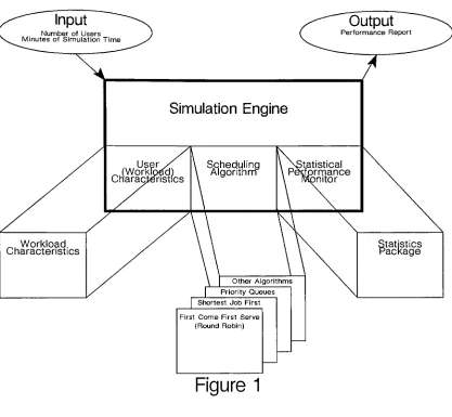
Project

Description

Input

NumberofUsers MinutesofSimulation Time

Output

Performance Report

Simulation

Engine

(Wortf>e._,

Characteristics

^,

Workload.

Characteristics

Scheduling

Algorithm

statistical

Performance ^nitor

Other Algorithms

PriorityQueues Shortest Job First

First Come First Serve (RoundRobin)

Figure

1

2.3.1.

The

Workload

Statistics Package

The

first

function

of the model

is

to generate an artificial workload that

simulates the

activity

of a specified number of users.

For

each user a series of "jobs"

must

be

generated which simulate the cycle of commands that a typical user

might

issue

(

edit,

list

files,

edit, compile, edit some

more, compile, run, print,

etc.).

The

workload

imposed

on the system will

be

controlled

by

adding

and

removing

"users"

and

examining

the variations

in

response time that occur.

Thus it

[image:27.529.46.463.93.478.2]

(28)

particular measurement

interval.

One

of the assumptions that the model makes

is

that user

behavior

is

homogeneous.

To

parameterize the

workload,

and

further define

the

behavior

of a typical

user,

data

was gathered

from

an

existing

time-sharing

user community.

A group

of

programmers

working

together on a software

development

project agreed to save

their "history"

files

which record the sequence of commands which

they

executed

during

their work session.

These

programmers are

working

on

Sun

Workstations,

which are

Motorola MC-68010 based

UNIX

system.

This

information

was gathered

by

having

each programmer provide a record of the system

load,

their

history

of

commands,

and the time

demands

of their work session.

This information

was

obtained

by

placing

several commands

in

the user's ".logout"

file.

The

"uptime" command

indicates

the number of users onthe system and the

relative

job

load.

This

command can

be

used to put a

time-stamp

on the

growing

master

history

file

and also

indicate

the number of users on the system as well as

the relative

job

load.

The

"history" command appends the

last

one

hundred

commands executed

by

each user

before

logging

off of the system.

The

"time"

command records the total amount of _user, system and real time utilized

by

that

user since the creation of their

login

shell.

From

this master collection of work

history

files

a

data

file

of typical

command execution sequences and relative

frequencies

was created.

This

listing

of

executed commands was analyzedto

determine

the relative

frequency

of occurence

of each command.

This

was

further

analyzedto plot the relative order of command

execution as atransition matrix.

If

the current

job is

"A",

what percent ofthe time

is

the subsequent

job

"B",

"C"

or

"D"? There

are typical sequences of commands

that users

frequently

execute.

For

example after

changing working

directories,

(29)

21

(

"Is"

in UNIX).

Similarly,

there are sequences of commands that are not

common.

A

user who

has just

completed compilation of a program

is

not

likely

to

recompile

immediately

without an

intervening

session of

further editing

or testing.

From

this analysis a

data file

was generated to represent these typical transitions.

This data file is

used

by

the

functions

which simulate

"typical

users"

to generate a

workload with a similar sequence and

frequency

of commands.

The

module that

generates the user workload exhibits

behavior

similar to the actual user

behavior,

as

just described.

One

of the

early

limitations

of

using

"history"

files

was that

only

the

last

twenty-five to

thirty

commands were

being

saved.

It

was

quickly

perceived that

there was a gradual evolution

in

the sequence of commands that a programmer

executes as the end of a work session

is

approached.

The

true sequence of

commands executed was not

being

captured

in

its

totality.

To

correct this problem

the users

later

maintained and reported a much

larger

personal

history

of one

hundred

commands.

When

a user's

job

is

created

by

the workload simulation module certain

things need to

be known

about that

job besides its

arrival time.

It

is

necessary

to

determine

the service requirements of this

job

based

on the

job

type.

To

parameterize this aspectof the simulated workload the

UNIX

"time"

function

was

used to measure the service requirements of a

large

sample of each of the

job

types that were

included

in

the

job

sequence and

frequency

database.

The

UNIX

"time"

function

returns the

following

information:

the amount of user

time,

system

time,

and real time used

in

the execution of _{the command; the} amount of

memory

used, the number of

I/O

interrupts;

and the amount of

paging

and

swapping

activity

associated with the timed process.

This

data

was recorded

for many

(30)

values allows typical service

demands

to

be

generated

for

each of the created user

jobs.

2.3.2.

The

"Simulation

Engine"

The

second

important

function

of the model could

be

called the

"simulation

engine".

The

overall control of the

simulation,

the

initialization

of _{the model,} and

the termination of the simulation are all controlled

by

this

"simulation

engine".

For

example,

the model

begins

by determining

how

many

users are to

be

simulated

in

this

iteration

and

how

many

minutes of simulated timethe model will continue to execute

before

printing

out the accumulated statistics.

The

simulation engine

has

to maintain a

"system

clock"

so that events can

be

scheduled, timed and recorded.

The

other major

responsibility

ofthis portion ofthe model

is

maintaining

and

manipulating

the

internal

queues of

jobs

in

various states which constitute the

inner

workings of the model.

The

first

of these

internal

queues contains the

"arriving

jobs" that are

being

submitted to our simulated processor

for

execution.

The

model must maintain a queue of

"future

events"

that will represent the

jobs

being

generated

by

the simulated users of the system.

The

module that simulates the user workload

is

responsible

for generating

the

jobs

that are entered

in

this queue.

The

second ofthese

internal

queues

is

the "ready-to-run" queue of

jobs

that

are

ready

and _waiting

for

cpu service.

Jobs

are moved

from

the queue of

"future

events"

into

the ready-to-run queue when their

designated

"arrival

time"

is

reached

by

the

inner

clock of the model which

keeps

track of simulated time.

The

job

to

be

scheduled

is

placed

into

the ready-to-run queue

according

to the

(31)

-23

-component of the model that

is easily

changed or exchanged to

implement

a

different

scheduling

algorithm.

The

"simulation

engine"

removes

jobs from

the ready-to-run queue and

"runs"

them.

As

jobs

move

from

one state to the next, time-stamps are

maintained

for

each

job

which allows the

gathering

of statistics

for

response

time,

execution

time,

and

waiting

time.

When

a

job finishes

running

these statistics are

gathered

from

the time-stamps

before

the

job

"leaves" the model.

The

termination

of a

job

will trigger the generation ofthe

"next

job"

for

that particular user which

is

then

be

placed

in

the queue of

future

events.

In

multi-process

time-sharing

computer systems

jobs

share the cpu with

other

jobs. When

a

job begins

service at the cpu

it does

not

necessarily finish

before

it

must give

up

use of the cpu to other

waiting jobs. The

quantum of time

allocated

by

the system

may

expire

before

the

job is

completed,

in

which case the

job

must

be

placed

back in

according

to the current

scheduling

algorithm.

The "simulation

engine"

is

responsible

for maintaining

this

sharing

of the cpu

time,

removing

jobs

from

the

running

state that

have

exceeded

the

designated

time quantum and are not yet

finished,

or are

blocked

waiting for

interactive keyboard input.

Jobs

in

the "blocked"

waiting

state are rescheduled as

future

events

due

to arrive at the time of their next calculated

"input".

The

first

scheduling

algorithm

implemented

is

a simple round-robin

scheduler where the

jobs

are placed

in

the ready-to-run queue on a

basis. The

second cpu

scheduling

algorithm

implemented

is

an optimal scheduler that can

be

represented

in

a model

but

not

in

reality

this

being

the shortest-remaining-time-first scheduler.

Since

time-stamps

are

being

maintained on each

job

it

will

be known

at all times what the

job's

total need

is,

(32)

would never

have in

a real computer

system,

it is

possible to schedule the

jobs in

order of their total unmet need

in

other words the shortest

job

first. A

third

algorithm to

be

examined maintains two ready-to-run

queues,

one

for "interactive

jobs"

and a second

for

"background" or "batch"

jobs. Interactive

jobs

will

be

run

first,

and when that queue

is empty jobs

will

be

run

from

the queue of

batch jobs.

The

flexibility

of the model allows

for

additional

scheduling

algorithms to

be

implemented

and tested with relative _ease,

but

shortest-job-first,

and

priority

queues are the three algorithms that will

be

analyzed

here.

2.3.3.

Coming

To Terms

The

model attempts to represent a user's perspective on the world.

Therefore

the performance parameter that this thesis

focuses

most

closely

on

is

system

response time.

I

am

using

response time to mean the elapsed time

from

the

job

submission time to

its

completion time.

I

believe

this

is

the

best

criterion

for

measuring

interactive

performance and most

closely

represents the user's

perception of system performance.

There

is

another

definition

of response time which measures the elapsed time

from

the submission of the

job

until the

first

appearance of response at the

terminal.

Often

the

first

appearance of a response will precede the completion of

the

job

by

a significant

interval. The first

appearance of response can

be very

reassuring

to the user that the system

is indeed

working

on the submitted

request,

particularly

when the

final

completion

may

take significant

fractions

of a minute or

longer. Some initial early

appearance of response

is reassuring

and

helps

prevent

impatient

users

from

re-submitting the

job

or

banging

on the

keys

to see

if

the

system

is

still

up

or responding.

I have

chosen not to use this second

definition

of

(33)

-25

In

the

inner

workings of the

model,

response time

is

measured as the

difference between

a

job's

arrival time and

its

departure

time.

A

job

is

assigned an

arrival time as

it is

placed

in

the

future-events

queue.

The

job

"arrives"

and

is

moved

into

the ready-to-run queue when the simulation clock

is

equal to or

greaterthan

its

scheduled arrival time.

If

a

job is

currently running

when the new

job is

scheduled to

arrive,

the

arriving

job

will

have

to wait until the

currently

active

job

completes

its

current cpu

burst.

Departure

time

is

marked when the

job

leaves

the cpu

for

the

last

time.

Departure

should occur when the total service

received

is

equal to the total service need that was

determined

when the

job

was

created

by

the

"User

and

Job

Demands

Module."

The

model also

keeps

track of cpu utilization and total throughput.

Total

cpu

utilization

is

the percentage of the total simulated time that the cpu was

actively

running

a user's

job.

Since

the system overhead associated with a user's

job is

combined with the usertime needed

for

a

job,

this cpu utilization

figure

could also

be

described

as the percentage of "non-idle" time.

The

throughput

is kept

as a

tally

of the total number of

jobs

completed

during

the period of simulation.

This

total can

be

divided

by

the number of minutes of simulation to arrive at a

jobs

completed per minute

figure. Throughput

and cpu utilization are good measures of

system performance,

however

response time

is

a

better indicator

of

how

the user

would experience or evaluate the system's

interactive

performance.

2.3.4.

Statistics

System

and

Job

of the model

is

to gather two categories of statistics.

Processor

utilization statistics are

kept

so that a system saturation workload

level

can

be

identified.

Statistics for

(or queues)

are maintained.

(34)

Histograms

describing

the population sizes of the ready-to-run queue

provide a _{graphical representation} _of _the _{size of}_the

waiting

queue overtime.

The

model

has been

designed

to report that

for

x amount of time there was one

job

waiting

to run, and

for

y

amount of time there were two

jobs

waiting

to _run,

etcetera.

The

model reports system population _statistics, so that a system

population of zero corresponds to the amount of time that the processor was

idle,

and a system population of one corresponds to those times when there was no

job

waiting

to run while a current

job

was

being

processed.

This

makes

it

possible to

calculate and report an average system population.

This

additional average system

population statistic

is

printed out

along

withthe

data

and

histogram

representations

of system population statistics.

The

second

namely interactive

jobs

such as

editing

),

and

what effect that optimization will

have

upon response times

for

other

job

types.

It

is

also

important

to

detect

whether

any

job

types are

being

starved out under

high

loads

with

any

of these algorithms.

In

the area of

job-related

statistics an additional measure of

job-related

system performance

is

reported.

Utilizing

average response times alone

does

not

allow meaningful comparisons to

be

made

between

the changes

in

response time

under

increasing

loads

of two

different

job

categories which

have

very

different

typical system demands.

For

example, an

editing

job

has

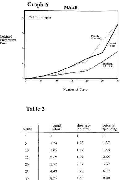
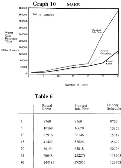
an average response time

of .042 seconds when there

is

a single user and

.261 seconds when there are

thirty

users on a system which utilizes round-robin scheduling.

How does

one compare

(35)

27

-averages

36.68

seconds

for

a single user and

increases

to

364.2

seconds when

there are

thirty

users

sharing

the system?

The difference

between

the system

demands

are so

different

for

these

job

categories that

it is

difficult

and perhaps

even meaningless to compare the

differential

changes

in

response time

between

these two

job

types on the

basis

of average response time.

While

average response time

is

still an

interesting

statistic to

look

_at,

weighted turn-around time

is

the measure of choice

for comparing

how jobs

of

different

types

fare

in

system performance.

[

Ferrari,

et. al.

1983

]

Weighted

turn-around time

is

the ratio

between

turn-around time and actual

processing

time.

On

a system with a single user this ratio should

be very nearly

equal to one

for

all

job

types.

The

time required

by

the system to process the

job is

divided into

the total turn-around time to yield a ratio that can

be

meaningfully

compared

across

job

categories.

These job

types

may differ widely in

the

demands

they

typically

place upon the system.

The

use of weighted turn-around time

is

of

further

help

in

diminishing

the

impact

of variations

in

system

demands

within a single

job

category.

All

compilations

do

not

have

the same

processing demands.

Weighted

turn-around

time yields a measure of system performance which takes these variations

in

processing demands into

account.

The

model reports statistics on weighted turn-around time.

When

the model

is

running

in

the

"verbose"

mode the weighted turn-around time

for

each

job is

reported as

it

completes execution.

The summary

job

statistics report

includes

the

mean weighted turn-around time

for

each

job

type.

The

mean weighted

turn-around time was

found

to

be

the most useful measure of system performance

for

the comparison of the

different scheduling

algorithms.

This

measure of system

(36)

performance of

scheduling

algorithms.

It

should

be

noted that weighted

turn-around time

is

particularly

sensitive to changes

in

shorter

duration

job

types.

2.4.

Limitations

of

the

Model

The

model

is

likely

to

be insensitive

to some of the

interactions

between

components of an actual computer system.

In

particular, the model will not

replicate some of the

thrashing

phenomena that

have

been

observed

in

paged

virtual

memory

computer systems as

they

approach saturation and there

is

a

dramatic increase

in

page

faults. The

present

design

of the model

does

not

directly

represent

memory

_contention,

swapping

or paging.

The

cpu overhead associated

with these activities

is

captured

in

the

"system

time"

component of the

UNIX

time

command that

is

being

used to calibrate this model.

So

while these activities are

not

directly

_represented, their

impact

upon system performance

is

taken

into

account.

The

model

does

not

separately

represent the

queuing

which occurs

for

disk

I/O.

The

times associated with this

queuing

are contained

in

the user and system

times generated

by

the

UNIX

time command.

The

model

factors

these

queuing

delays into

the total

delays

that the user perceives as response time.

Questions

about the

interaction between

a given cpu

scheduling

algorithm and the

intensity

of

I/O activity

cannot

be

answered

by

this model.

An

avenue

for future

exploration

and enhancement of the model might

be

to take

disk

I/O queuing into

account

directly.

It

would then

be

possible to examine

queuing

algorithms which give

differential treatment to

I/O bound

and compute

bound

jobs.

It is

likely

possible

that

further

control and

tuning

of response time could

be

obtained

by

differential

(37)

-29