THE TRANSFORM AND DATA COMPRESSION HANDBOOK K R RAO pdf

(1)

The Transform and Data Compression Handbook

Ed. K. R. Rao and P.C. Yip.

(2)

THE

TRANSFORM

AND DATA

COMPRESSION

(3)

THE ELECTRICAL ENGINEERING

AND SIGNAL PROCESSING SERIES

Edited by Alexander Poularikas and Richard C. Dorf

Handbook of Antennas in Wireless Communications

Lal Chand Godara

Propagation Data Handbook for Wireless Communications

Robert Crane

The Digital Color Imaging Handbook

Guarav Sharma

Handbook of Neural Network Signal Processing

Yu Hen Hu and Jeng-Neng Hwang

Handbook of Multisensor Data Fusion

David Hall

The Advanced Signal Processing Handbook:

Theory and Implementation for Radar, Sonar,

and Medical Imaging Real Time Systems

Stergios Stergiopoulos

The Transform and Data Compression Handbook

K.R. Rao and P.C. Yip

The Encyclopedia of Signal Processing

Alexander Poularikas

(4)

Boca Raton London New York Washington, D.C. CRC Press

THE

TRANSFORM

AND DATA

COMPRESSION

HANDBOOK

Edited by

K.R. RAO

University of Texas at Arlington

AND

(5)

This book contains information obtained from authentic and highly regarded sources. Reprinted material is quoted with permission, and sources are indicated. A wide variety of references are listed. Reasonable efforts have been made to publish reliable data and information, but the author and the publisher cannot assume responsibility for the validity of all materials or for the consequences of their use.

Neither this book nor any part may be reproduced or transmitted in any form or by any means, electronic or mechanical, including photocopying, microfilming, and recording, or by any information storage or retrieval system, without prior permission in writing from the publisher.

All rights reserved. Authorization to photocopy items for internal or personal use, or the personal or internal use of specific clients, may be granted by CRC Press LLC, provided that $.50 per page photocopied is paid directly to Copyright Clearance Center, 222 Rosewood Drive, Danvers, MA 01923 USA. The fee code for users of the Transactional Reporting Service is ISBN 0-8493-3692-9/00/$0.00+$.50. The fee is subject to change without notice. For organizations that have been granted a photocopy license by the CCC, a separate system of payment has been arranged.

The consent of CRC Press LLC does not extend to copying for general distribution, for promotion, for creating new works, or for resale. Specific permission must be obtained in writing from CRC Press LLC for such copying.

Direct all inquiries to CRC Press LLC, 2000 N.W. Corporate Blvd., Boca Raton, Florida 33431.

Trademark Notice: Product or corporate names may be trademarks or registered trademarks, and are used only for identification and explanation, without intent to infringe.

No claim to original U.S. Government works International Standard Book Number 0-8493-3692-9

Library of Congress Card Number 00-057149

Printed in the United States of America 1 2 3 4 5 6 7 8 9 0 Printed on acid-free paper

Library of Congress Cataloging-in-Publication Data

The transform and data compression handbook / editors, P.C. Yip, K.R. Rao. p. cm.--(Electrical engineering and signal processing series) Includes bibliographical references and index.

ISBN 0-8493-3692-9 (alk. paper)

1. Data transmission systems--Handbooks, manuals, etc.. 2. Data compression (Telecommunication)--Handbooks, manuals, etc. I. Yip, P.C. (Pat C.) II. Rao, K. Ramamohan (Kamisetty Ramamohan) III. Series

TK5105 .T72 2000

(6)

Preface

While this handbook is an exposition of different discrete transforms and their ever-expanding applications in the general area of signal processing, the overriding task is to maintain the continuity and connectivity among the chapters. This task is accom-plished by the common theme of data compression. The handbook seeks to provide the reader with a wealth of information regarding the transforms (some have been widely used while others have great potential) as well as a demonstration of their power and practicality in data compression. Such compression is a necessary and desirable ingredient in today’s world of massive data storage and data transmission. By providing a plethora of Web sites, ftp locations, and references to general review papers, the chapter authors have expanded the usefulness of this handbook for the common reader. The clear and concise presentations of the ideas and concepts, as well as the detailed descriptions of the algorithms, provide important insights into the applications and their limitations. With the understanding of these concepts, readers can apply the techniques presented in this handbook to their own areas of interest and improve on the performance by marrying this with their own expertise. We are confident that this handbook will be a valuable addition to the bookshelf of anyone actively engaged in or studying the art and science of signal processing.

(7)

(spa-tial/temporal) and multiquality (SNR) end products, subject to bandwidth limitation, processing power, and cost constraints.

Many international standards relating to audio, video, and data, such as JPEG, H.261, H.262, MPEG-1, MPEG-2, MPEG-4, HDTV, and JPEG-2000, utilize trans-forms in their overall compression schemes. A number of consumer and commercial products, such as video-CD, DVD, videophone, set-top boxes, digital TV, and digital camera/VCR, have been made possible because of signal compression. Other elec-tronic innovations, such as MP3, video-streaming, and wireless PCS, are completely dependent on the reduction of bit rates made possible by compression. It is not ex-aggerating to say that data compression is one of the main contributing factors in the explosive growth in information technology.

While different coding schemes can accomplish an amazing amount of compres-sion, the cornerstone is still undoubtedly the underlying transform. It is for this reason that the definitions and properties for each of the transforms dealt with in this hand-book are presented with such care and detail. The bibliography sections and Web sites provide further sources of information.

Outline of Chapters

Chapter 1 The Karhunen-Loève Transform

The first transform described in this handbook is the Karhunen-Loève transform (KLT). It takes its rightful place as the leadoff transform to be discussed. Dony does an excellent job of interpreting this statistically optimal transform. The simple and yet elegant explanation of rotation of axes in the data domain to achieve the “principal components” representation underscores the significant energy compaction provided by this transform. Other properties of the transform follow, and the chapter is rounded off with descriptions of applications in chest radiographs and other monochrome and color images. Web sites and software download locations are listed as well.

Chapter 2 The Discrete Fourier Transform

(8)

Chapter 3 Comparametric Transforms for Transmitting Eye Tap Video with Picture Transfer Protocol (PTP)

This is a unique, challenging, and provocative chapter written by Mann, the inven-tor of the wearable computer (WearComp), the Eye Tap camera, and reality mediainven-tor. This chapter takes us to the forefront of the multimedia revolution with a new compu-tational/communications device that subsumes the functionality of the videophone, digital camera, and other wireless personal electronics innovations. Mann’s invention functions as a true extension of the mind and body and causes the eye to function as if it were a camera. His invention has given rise to a whole new philosophical and mathematical approach to image compression and image storage, and it gives a refreshingly new definition of functionality in image transmission and processing. The new Eye Tap genre of video is best processed and compressed by comparametric equations, essentially equations representing projections and tone scale adjustments of images. Traditionally image compression has been directed to ensure a certain minimum quality or reliability (e.g., worst case scenario). The author instead makes a compelling argument in favour of “best case” scenario; Mann argues that being able to broadcast even intermittent still images to the Internet can provide a measure of security unmatched by conventional “robust” security systems. These arguments are based on a definition of “fear of functionality,” a completely novel approach to the idea of security. The author has set up a Web site from which computer programs can be freely downloaded. Such a generous spirit is to be commended. It is also inter-esting to note that this chapter was typeset using LaTex running on a small wearable computer designed and built by the author.

Chapter 4 Discrete Cosine and Sine Transforms

Next to the DFT, discrete cosine transform (DCT) is probably the most used trans-form in digital signal processing work. DCT is one of a family of trigonometric transforms including the discrete sine transform (DST). In this chapter, Britanak presents a unified treatment of the family of DCTs and DSTs starting with the def-initions, properties, and fast algorithms. This chapter is particularly relevant as the DCT has been adopted in several international standards for image/video coding. In modified form, both DCT and DST have been used in MDCT/MDST audio coding. Computer programs in C (listed in Sections 4.3 and 4.4) that can be implemented to perform the transforms are very useful in all signal processing applications. The chapter concludes with a specific application in a Joint Photographic Experts Group (JPEG) base line system (Fig. 4.3) using the standard test image of Lena.

Chapter 5 Lapped Transforms for Image Compression

(9)

described. Generalized versions of the lapped orthogonal transform (LOT), called GenLOT, are developed in Sections 5.6.3–4 while cosine-modulated LTs, otherwise known as MLT or ELT, are discussed in Section 5.8. To demonstrate the promise and potential for LTs in image coding, well known image compression algorithms are applied to standard test images, with DCT or the wavelet transform replaced by LTs. Comparative analysis shows the elimination of ringing and blocking artifacts that are characteristic of the DCT based coders and also performance rivaling that of the wavelet transforms.

Chapter 6 Wavelet-Based Image Compression

This is another highly valuable chapter as it addresses wavelet-based image com-pression. Wavelet-based transforms give a time-frequency decomposition of the sig-nal, which has multi-resolution characteristics. The transforms have superior energy compaction and compatibility with Human Visual System (HVS). They make possi-ble the embedded bit-stream coding corresponding to various subbands (the basis for fast browsing of images or databases over the Internet). Discrete wavelet transforms (DWT) and its variants have been adopted both by the FBI in the use of fingerprint image compression and the international standards groups (JPEG-2000 and MPEG-4 still frame image coding). It is highly possible that wavelets may eventually replace DCT in all the coders. Walker and Nguyen provide a clear explanation of the mul-tiresolution aspects of DWT and its implementation using a 2-channel filter bank. Some of the recent enhancements of the basic DWT, such as EZW, SPIHT, WDR, and ASWDR, are enumerated, followed by their implementation in image coding and subsequent evaluation. Various Web sites that provide software, literature, simulation results, and innumerable other details further strengthen the chapter’s utility.

Chapter 7 Fractal-Based Image and Video Compression

(10)

Chapter 8 Compression of Wavelet Transform Coefficients

The concluding chapter presents a philosophical and thoughtful argument for the effectiveness of transforms in general and wavelets in particular for bandwidth re-duction. The superiority of wavelet transform over others, including the widely used DCT, is clearly demonstrated by the characteristics of the DWT. From the chapter’s title, the reader may get a wrong impression of duplication with Chapter 6. On the contrary, this chapter complements the topics in Chapter 6 by a clear exposition of the superior performance of the DWT over other transforms. The subband decom-position inherent in dyadic wavelet transform, preservation of spatial signal features in subbands of different scales, and self similarities among subbands of the spatial orientation are some of the reasons for this superiority. These self-similarities are conducive to statistical context modeling and adaptive entropy coding of wavelet co-efficients. By a lucid presentation of these concepts aided by implementation on test images, Wu convincingly demonstrates the validity of the DWT adopted in JPEG-2000 and MPEG-4 and the bright future it has in other applications.

Acknowledgements

(11)

List of Acronyms

AFB Analysis filter bank

ASPEC Audio spectral perceptual entropy coding ASWDR Adaptively scanned wavelet difference reduction bpp Bits per pixel

CREW Compression by reversible embedded wavelets DCT Discrete cosine transform

DFT Discrete Fourier transform DPCM Differential pulse code modulation DSP Digital signal processing

DST Discrete sine transform DTFT Discrete time Fourier transform DWP Discrete wavelet packet DWT Discrete wavelet transform

ECECOW Embedded conditional entropy coding of wavelet ECG Electrocardiogram

ELT Extended lapped transform EZC Embedded zerotree coding EZW Embedded zerotree wavelet FAQ Frequently asked questions FFT Fast Fourier transform FIR Finite impulse response FLT Fast lapped transform FoF Fear of functionality

FPGA Field programmable gate array GenLOT Generalized LOT

GNU GNU’s Not Unix

GNUX GNU-Linux

H.261 Standard for compression of videotelephony and teleconferencing H.263 Standard for visual communication via telephone lines

HDTV High definition TV

HLT Hierarchical lapped transform HSI Hue, saturation, intensity HV Horizontal vertical HVS Human visual system

(12)

ISO International Standards Organization ITU International Telecommunication Union JBIG Joint Binary Image Group

JPEG Joint Photographic Experts Group JPEG-LS JPEG-Lossless

KLT Karhunen-Loève transform LBT Lapped bi-orthogonal transform LOT Lapped orthogonal transform

LT Lapped transform

LZC Layered zero coding MC Motion compensated

MDCT Modified discrete cosine transform MDST Modified discrete sine transform MIMO Multi-input multi-output MLT Modulated lapped transform MOS Mean opinion score

MP3 MPEG-Layer 3

MPEG Moving Pictures Expert Group MPEG-AAC MPEG advanced audio coder MSE Mean squares error

PAC Perceptual audio coder PCA Principal component analysis PIFS Partitioned iterated function systems PR Perfect reconstruction

PSD Personal safety device PSNR Peak signal to noise ratio PTM Polyphase transfer matrix PTP Picture transfer protocol

QCLS Quadratic-constrained least squares

QM Cute sound

QPIFS Quadtree partitioned iterated function systems RGB Red, green, and blue

RLC Run-length coding RLD Run-length decoder ROI Region of interest RTT Round trip time

SDF Symmetric delay factorization SFB Synthesis filter bank

SPIHT Set partitioning of hierarchical tree STW Spatial orientation tree wavelet SVD Singular value decomposition TDAC Time domain aliasing cancellation

TF Time-frequency

VLC Variable-length coding VLD Variable-length decoder VQ Vector quantization WDR Wavelet difference reduction

(13)

Contributors

Vladimir Britanak Institute of Control Theory and Robotics, Slovak Acad-emy of Sciences, Bratislava, Slovak Republic

Ricardo L. de Queiroz Digital Imaging Technology Center, Xerox Corpora-tion, Webster, New York

R.D. Dony School of Engineering, University of Guelph, Guelph, Ontario, Canada

Guojun Lu Gippsland School of Computing and Information Technology, Monash University, Churchill, Victoria, Australia

Steve Mann Department of Electrical and Computer Engineering, Univer-sity of Toronto, Toronto, Ontario, Canada

Truong Q. Nguyen Department of Electrical and Computer Engineering, Boston University, Boston, Massachusetts

Gerald Schuller Bell Labs, Lucent Technologies, Murray Hill, New Jersey

Ivan W. Selesnick Department of Electrical Engineering, Polytechnic Uni-versity, Brooklyn, New York

Trac D. Tran Department of Electrical and Computer Engineering, The Johns Hopkins University, Baltimore, Maryland

James S. Walker Department of Mathematics, University of Wisconsin-Eau Claire, Eau Claire, Wisconsin

(14)

The Transform and Data Compression Handbook

Ed. K. R. Rao and P.C. Yip.

(20)

Chapter 1 Karhunen-Loève Transform

R.D. Dony

University of Guelph

1.1 Introduction

The goal of image compression is to store an image in a more compact form, i.e., a representation that requires fewer bits for encoding than the original image. This is possible for images because, in their “raw” form, they contain a high degree of redun-dant data. Most images are not haphazard collections of arbitrary intensity transitions. Every image we see contains some form of structure. As a result, there is some cor-relation between neighboring pixels. If one can find a reversible transformation that removes the redundancy by decorrelating the data, then an image can be stored more efficiently. The Karhunen-Loève Transform (KLT) is the linear transformation that accomplishes this.

In Section 1.2 we show how pixels are correlated in typical images. With the pixel values forming the axes of a vector space, a rotation of this space can remove this correlation. The basis vectors of the new space define the linear transformation of the data. The basis vectors of the KLT are the eigenvectors of the image covariance matrix. Its effect is to diagonalize the covariance matrix, removing the correlation of neighboring pixels.

(21)

1.2 Data Decorrelation

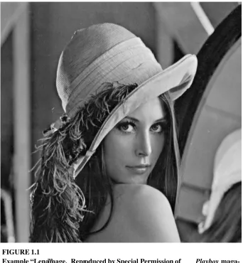
Data from neighboring pixels are highly correlated for most images.Fig. 1.1shows a typical gray scale image. The image is 512×512 pixels in size with each gray level brightness value of pixel being represented by an 8-bit value for a range of [0–255]. This particular image is commonly used in evaluations and is often referred to as the Lena image. Even with a large degree of detail in many regions, the gray level value of any given pixel tends to be similar to its neighboring pixels. To illustrate this relationship, one can plot the gray level values of pairs of adjacent pixels as shown inFig. 1.2. Each dot represents a pixel in the image with thexcoordinate being its gray level value and theycoordinate being the gray level value of its neighbor to the right. The strong diagonal relationship about thex =yline clearly shows the strong correlation between neighboring pixels.

If we were to block the image into nonoverlapping 1×2 pixel blocks as shown in

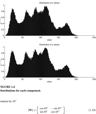
Fig. 1.3,we can represent an image by a collection of two-dimensional vectorsx_i. The scatter plot of this collection is equivalent toFig. 1.2.Looking at the distributions of the values for each of the two components as shown inFig. 1.4, we see that they are relatively wide and cover most of the 0–255 range. In fact, the distributions of each component would be quite similar to the overall distribution of individual pixels in the image.

Now, what would happen if we rotated the distribution shown in Fig. 1.2 by 45◦ about the center? The result is shown inFig. 1.5. The two components are now decorrelated, i.e., knowing the value of the first component does not help in estimating the value of the second. The distributions of the new components are shown inFig. 1.6. The first component, save for the shift and a scaling factor of√2, is still quite similar to the previous distributions — quite broad and covering most of the dynamic range of the original individual pixels. The second component, however, is quite different. It is much narrower, with a strong peak at 0. Because it has a smaller dynamic range, we could encode its value with fewer bits. So even with a decorrelation by a simple rotation of the axis, we can reduce the number of bits required for encoding an image. In general, a process is decorrelated when, for zero mean random variablesx_i and xj, the expectation of their product, the covariance, is zero ifi=j, i.e.,

Exixj=

0 i=j , σ2

i i=j , (1.1)

whereE(·)is the expectation operator. Using vector notations, we may define the vector of the values of an image block ofNpixels as

x=[x1x2 . . . xN]T . (1.2)

We can then define the covariance matrix as

[C]_x=E

(x−m) (x−m)T

(22)

[image:22.612.104.446.127.497.2]

FIGURE 1.1

wherem=E(x)is the mean. For notational convenience, we will assume zero mean input for the rest of this chapter. In practice, the mean can simply be removed from the data before processing.

We wish to find a linear transformation matrix,[W], whose transpose,[W]T, will rotatexto produce a diagonal covariance matrix for the transformed variabley,

y= [W]Tx. (1.4)

Each column vector,w_i, of[W]is a basis vector of the new space. So, alternatively, each element,y_i, ofyis calculated as

(23)

[image:23.612.159.488.135.470.2]

FIGURE 1.2

Scatter plot of adjacent pixel value pairs.

For simple rotations with no scaling, the matrix[W]must be orthonormal, that is

[W]T[W] = [I] = [W][W]T (1.6)

where[I]is the identity matrix. This means that the column vectors of the matrix are mutually orthogonal and are of unit norm. From Eq. (1.6), it follows that the inverse of an orthonormal matrix is simply its transpose, [W]T = [W]−1. The inverse transformation is then calculated as

(24)

[image:24.612.109.444.128.380.2]

FIGURE 1.3

Image blocking with1×2pixel nonoverlapping blocks.

Further, the total energy under the transformation is preserved

y2=yTy

=[W]Tx _T

[W]Tx

=xT[W][W]Tx

=xTx

= x2 ,

(1.8)

wherexis the norm of the vectorxdefined as

x =

xTx

=

N

i=1 x2

i .

(1.9)

(25)

[image:25.612.163.497.126.522.2]

FIGURE 1.4

Distributions for each component.

rotation by 45◦

[W] =

cos 45◦ −sin 45◦ sin 45◦ cos 45◦

. (1.10)

For an arbitrary covariance matrix, the problem of finding the appropriate transfor-mation is the orthonormal eigenvector problem. Since the covariance matrix is real and symmetric, we can find its real eigenvalues and corresponding eigenvectors. Let

[C]_ybe the desired diagonal covariance matrix of the transformed variableywhich will be of the form

[C]_y=   

λ1 0

...

0 λ_N

 

 , (1.11)

(26)

--

-

-FIGURE 1.5

Scatter plot of pixel value pairs rotated by 45◦.

matrix can be calculated from the original covariance matrix,[C]_x, as

[C]_y=E

yyT

=E[W]Tx [W]Tx _T

=E[W]T

xxT

[W]

= [W]T[C]_x[W],

(1.12)

or equivalently,

[image:26.612.104.437.117.481.2]

(27)

-FIGURE 1.6

Distributions for each component of the rotated pixel value pairs.

Since the desired[C]yis diagonal, Eq. (1.13) can be rewritten for each column vector,

w_i, of[W]as

[C]_xw_i =λ_iw_i . (1.14)

The solutions forλ_i andw_i withi =1, . . . , N in Eq. (1.14) are theN eigenvalue, eigenvector pairs of the matrix[C]_x of dimension N ×N. That is, each column vector of[W]is an eigenvector of the covariance matrix,[C]_x, of the original data. To ensure that[W]is orthonormal, Gram-Schmidt orthogonalization may be applied to the eigenvectors as they are obtained.

(28)

1.2.1 Calculation of the KLT

Estimation of Covariance

The calculation of the KLT is typically performed by finding the eigenvectors of the covariance matrix, which, of course, requires an estimate of the covariance matrix. If the entire signal is available, as is the case for coding a single image, the covariance matrix can be estimated fromndata samples as

[C]x= 1_n n

i=1

xixT_i , (1.15)

wherex_i is a sample data vector. If only portions of the signal are available, care must be taken to ensure that the estimate is representative of the entire signal. In the extreme, if only one data vector is used then only one nonzero eigenvalue exists, and its eigenvector is simply the scaled version of the data vector. For typical images, it is rarely the case that their covariance matrix has any zero eigenvalues. For a data vector of dimensionN, a good rule of thumb is that at least 10×N representative samples from the various regions within an image be used to ensure a good estimate if it is not feasible to use the entire image.

Calculation of Eigenvectors

While it is beyond the scope of this chapter to provide a detailed discussion of the algorithms for extracting the eigenvalues and eigenvectors, we will present a brief overview of the general methods commonly used. The reader is referred to [16, 28] for more detailed explanations. For actual implementations of the methods, many numerical packages such as LAPACK [22] (which is based on EISPACK [21] and LINPACK [23]), MATLAB [20], IDL [31], and Octave [11], and the routines in “cookbooks,” such as that by Press et al. [28], provide routines for the solution of eigensystems.

A simple approach is the Jacobi method. It develops a sequence of rotation matrices,

[P]_i, that diagonalizes[C]as

[D] = [V]T[C][V], (1.16)

where[D]is the desired diagonal matrix and[V] = [P]1[P]2[P]3· · ·. Each[P]_i

rotates in one plane to remove one of the off-diagonal elements. It is an iterative technique which is terminated when the off-diagonal values are close to zero within some tolerance. Upon termination, the matrix [D]contains the eigenvalues on the diagonals and the columns of[V]are the basis vectors of the KLT.

(29)

of this approach is that the factorization on the simplified tridiagonal matrix typically requires fewer iterations than the Jacobi method.

Recently, there has been some interest in iterative methods of principal components extraction that do not require the calculation of a covariance matrix [7, 14, 26]. These techniques update the estimate of the eigenvectors for each input training vector. One such method developed by Oja [25] is of the form

ˆ

w(t+1)= ˆw(t)+α

y(t)x(t)−y2(t)wˆ(t)

, (1.17)

wherexis an input vector,wˆ(t)is the current estimate of the basis vector,y=wTx

is the coefficient value, and α is a learning-rate parameter. Eq. (1.17) has been shown to converge to the largest principal component [14, 27]. This algorithm can be generalized through deflation to extract any or all of the principal components [7, 33]. Also, adaptive schemes have been based on this method [8]. While these algorithms have some advantages over covariance-based methods, there are still some concerns over stability and convergence [3, 4, 35].

Markov-1 Solution

The calculation of the eigenvectors for an arbitrary covariance matrix can still require a large number of computations. However, there is a special class of matrix that has an analytical solution for its eigenvectors and eigenvalues [29, 30]. If a process were to have a covariance function of the form

[C]_ij =σ2ρ|i−j|, (1.18)

whereρis the correlation coefficient such that 0< ρ <1, such a process is referred to as a first order stationary Markov process or simply Markov-1. The solution for theith element of thejth basis vector forN-dimensional data is given by

wij =

2

N+µj 1_/2

sin

rj

(i+1)−(N+1) 2

+(j+1)π 2

, (1.19)

whereµ_j is thejth eigenvalue calculated as

µj =

1−ρ2 1−2 cosr_j+ρ2

, (1.20)

andr_j is thejth real positive root of the transcendental equation

tan(Nr)= −

1−ρ2_sin_(r)

cos(r)−2ρ+ρ2_cos_(r) . (1.21)

(30)

Then, thei, jelement of thekth two-dimensional basis vector,w_ijk, is calculated as the product of the two:

wijk =wik(H)wjk(V ). (1.22)

As many images exhibit a Markov-1 structure, this solution to the KLT can be quite useful due to its ease of generation.

1.3 Performance of Transforms

On its own, an orthonormal transformation does not effect data compression. The blocks of pixels are simply transformed from one set of values to another and, for reversible transformations, back again on reconstruction. To reduce the number of bits for representing an image, the coefficients are quantized, incurring some irreversible loss, and then encoded for more efficient representation. By decorrelating the data before these steps using the KLT, more data compaction can be achieved.

To examine the effects of this extra efficiency, we can make use of Shannon’s information measures [34].

1.3.1 Information Theory

The information conveyed by an observation of some random process is related to its probability of occurrence. If an observation were all but certain to occur, i.e., its probability were close to 1, it would not be very informative. However, if it were quite unexpected, the observation would convey much more information. Shannon formalized this relationship between the probability of an event,P (x), and its information content,I (x), as

I (x)= −logP (x) . (1.23)

If the logarithm is taken with respect to base 2, the information,I (x), is measured in units ofbits.

A random variable, x, is a collection of all possible events and their associated probabilities. The average information for a random variable can be calculated as

H (x)= i

P (xi) I (xi)

= −

i

P (xi)logP (x_i) ,

(1.24)

(31)

Entropy is useful in determining theoretical performance measures of compression methods. Shannon showed that entropy gives a lower bound on the average number of bits required to encode the events of a random process without introducing error. In other words, one needs at least as many bits per event, on average, as the entropy to represent a set of observations.

However, these measures are not directly applicable to the coefficients of an arbi-trary transformation. They are defined for discrete events whereas the coefficients, since they are floating-point values, must be considered real-valued samples of con-tinuous distributions. Since the probability of any such real-valued sample is zero, the (discrete) entropy is undefined. Instead, we define thedifferential entropy[13] as

h(x)= −

_∞

−∞p(s)logp(s)ds . (1.25)

For simple distributions such as the Gaussian, uniform, or Laplacian distributions the differential entropy is of the form

h(x)=1

2logσ

2

x +k , (1.26)

whereσ_x2is the variance of the random variable andkis a distribution-dependent constant (e.g., for a Gaussian,k= 1₂log₂2πe) [1].

A good transformation, then, should minimize the sum of the differential entropies for the resulting coefficients. Due to the logarithmic term, this is equivalent to mini-mizing the product of the variances of the coefficients. However, recall that for any orthonormal transformation, the total energy is preserved, so the sum of the coeffi-cient variances is fixed. One measure of the efficiency of the transform is the coding gain [10] defined as the ratio between the algebraic mean of the variances, which is independent of the transform, and the geometric mean of the variances, which is transform dependent:

GW =

1 N

N

i=1 σ2

yi _N

i=1 σ2

yi

1/N . (1.27)

For the raw signal, before any transformation, all the variances are approximately equal giving a unity coding gain. Any increase in one of the coefficient variances must be matched by an equal decrease in one or more of the other variances for an orthonormal transform. The arithmetic mean is therefore the same, but the geometric mean decreases resulting in a coding gain of greater than one.

(32)

coefficient. Next, subject to the orthonormality constraint, maximize the variance of the second coefficient, and so on. This procedure is nothing more than extracting the principal components or, equivalently, generating the KLT. Therefore, the KLT, by decorrelating the data, produces a set of coefficients that minimizes the differential entropy of the data.

1.3.2 Quantization

In transform coding, the transform coefficients are quantized to effect the data reduction. While the transformation is reversible, quantization is not, and therefore introduces error. Letyˆ be the set of quantized coefficient values for a block. On reconstruction, the block is calculated as

ˆ

x= [W]ˆy. (1.28)

The squared error for the block is calculated as

ε2₌_x_ˆ₋_x2

=xˆ−xT xˆ−x

=[W]ˆy− [W]yT [W]ˆy− [W]y

=yˆ−yT [W]T[W]yˆ−y

=yˆ−yT yˆ−y

=yˆ−y2 .

(1.29)

So, the squared error on reconstruction is the same as the squared error of the coeffi-cients for orthonormal transformations.

The quantized coefficients are typically encoded using a lossless method, such as arithmetic coding or Huffman coding. These methods can, at best, reduce the average number of bits to the entropy of the quantized coefficients.

To illustrate the advantage of performing the KLT before quantization, we calculate the total entropy for a number of quantization intervals on both the original data and the transformed data. For this example, a midstep, uniform quantizer is used where the quantized value is calculated as

ˆ

y=qround(y/q) , (1.30)

based on the width of the quantization interval, q, where the function round(x) returns the nearest integer to the real valuex. The results are shown inFig. 1.7. For a given squared error due to quantization, the entropy in bits per pixel is less for the transformed data than for the original data.

1.3.3 Truncation Error

(33)

FIGURE 1.7

Plot of mean squared error (MSE) versus entropy in bits per pixel for a number of quantization widths.

Eε2 ₌ _E

1 N

N

i=1

yi− ˆyi2

= 1

NE  M

i=1

(yi−yi)2+ N

i=M+1

(yi−0)2



 (1.31)

= _N1E   N

i=M+1 y2

i  

= 1

N N

i=M+1 σ2

i .

(34)

Notice that the above minimization is valid for any transformation whoseMbasis vectors span theM-dimensional subspace defined by theMlargest principal compo-nents (eigenvectors for theMlargest eigenvalues). However, only the KLT ensures that the remaining coefficients can be coded with the minimum number of bits since it minimizes the differential entropy of the coefficients. To illustrate this point, let us generate the 64 KLT basis vectors for an 8×8 blocking of the test image and keep only the first four. The variances of the resulting coefficients are shown in the first column of Table 1.1. The MSE due to the removal of the 60 lowest variance coefficients is 96.1. Now, let us generate another set of 4 basis vectors by taking random linear combinations of the first 4 KLT basis vectors. The new set still spans the space defined by the original 4 KLT basis vectors. As a result, the MSE due to truncation and the sum of the remaining variances are identical to those of the KLT bases. However, the product of the variances is much higher, and, as a result, the coding gain is much smaller than for the KLT bases. This means that the representa-tion is less efficient and will require more bits to encode the coefficients for the same degree of distortion.

Table 1.1

Performance Differences Between First Four Basis Vectors of KLT and a Random Combination of Them

KLT bases Random span

σ2

1 113995 20876

σ2

2 6880 18236

σ2

3 2727 79310

σ2

4 1691 6873

4

i=1 σ2

i 125294 125294

64

i=5 σ2

i 6147 6147

Truncation MSE 96.1 96.1

4

i=1 σ2

i 3.6×1015 207.5×1015

Coding gain 4.04 1.47

1.3.4 Block Size

(35)

of arithmetic operations for the forward and inverse transformations increases linearly with the number of pixels in the block. Furthermore, the size of the covariance matrix is the square of the number of pixels. Not only does the calculation of the eigenvectors require more resources, but the number of samples to get a reasonable estimate of the covariance matrix increases significantly. As well, if the set of KLT basis vectors is to be kept with the image for reconstruction, the size of the basis set is also of concern. Therefore, there is a trade-off between computational requirements and the degree of decorrelation in determining the block size.

Fig. 1.8shows the coding gain as a function of block size for the test image. It clearly shows that the use of larger block sizes results in larger coding gains. For example, increasing the block size from 4×4 to 8×8 increases the gain from 27 to 39. However, the number of floating point operations per pixel increases by a factor of four from 32 to 128.

FIGURE 1.8

(36)

Of course, using a block the same size as the image results in a perfect coding gain since the entire image can be represented by a single component. Unfortunately, this representation is so image specific that the transform basis itself must also be included with the compressed image to enable reconstruction. Since the basis vector

isthe image, one is no further ahead. However, such full-frame transform coding may be appropriate for sequences or collections of similar images.

Interblock Correlation

The KLT produces decorrelated coefficients within the image blocks. There is no assurance, however, that the coefficients from block-to-block are also decorrelated. In fact, for most images there is a significant correlation between the first coefficients for adjacent blocks. For example,Fig. 1.9shows the scatter plot of adjacent pairs of the first coefficient for the 8×8 KLT of the test image. Note the strong correlation between the adjacent values. In contrast, Fig. 1.10shows little if any correlation between adjacent second coefficients.

A simple method of reducing such correlation is to encode only the difference between adjacent coefficients after initially encoding the first. This method is known as differential pulse code modulation (DPCM). The use of DPCM on the first coeffi-cients significantly increases the overall coding efficiency by reducing the variance of the coefficient. For example, performing DPCM on the first coefficient of the above 8×8 KLT coefficients reduces the variance from 113995 to 51676. The resulting scatter plot of the adjacent pairs of differences is shown in Fig. 1.11. The use of DPCM has removed the correlation between adjacent values of the first coefficient.

1.4 Examples

1.4.1 Calculation of KLT

To calculate the KLT of an image, the covariance matrix is first estimated. The estimate is calculated from the set of sequential nonoverlapping blocks for the image. For the following examples, blocks of 8×8 pixels are used. For the “Lena” image, this results in 4096 blocks. The eigenvalues and the corresponding eigenvectors are extracted from the covariance matrix. Because the matrix is symmetric, the eigenvalues and eigenvectors can be calculated using the tridiagonalization and QL factorization approach.

The resulting 64 basis vectors are shown in Fig. 1.12as two-dimensional basis images or blocks. The bases are in order from the largest variance at the top left to the lowest at the bottom right. Dark pixels represent negative values and light pixels represent positive values. The first basis is almost flat due to the similarity of pixel values within most blocks. As was the case for the two-dimensional scatter plot of

(37)

--

-

-FIGURE 1.9

Scatter plot of adjacent pairs of the first coefficient.

first component of the KLT tends to be constant or d.c. As the variance increases, the degree of variation, or frequency, increases. This relationship generally agrees with the form of the KLT solution for a Markov-1 process as shown in Eq. (1.19) where the frequency increases as the basis index increases. Again, as most images have an approximate Markov-1 structure, the form of the KLT bases are similar.

1.4.2 Quantization and Encoding

(38)

--

-

-FIGURE 1.10

Scatter plot of adjacent pairs of the second coefficient.

same quantization step size,q, is used for all coefficients, unlike the JPEG standard that varies the degree of quantization for each coefficient according to the visibility of error as judged by human observers. Each quantized coefficient is encoded first by a Huffman encoded value for the number of bits required by the coefficient followed by the minimum number of bits for the coefficient value itself. Zero-valued coefficients from adjacent blocks are run-length encoded for further compaction.

(39)

--

-

-FIGURE 1.11

Scatter plot of adjacent pairs of differences of the first coefficient.

As the bit-rate decreases, distortion increases. Table 1.2shows the distortion in two equivalent common measures [6]. The mean squared error (MSE) is defined as

MSE=Ex− ˆx2

, (1.32)

wherexis the original pixel value andxˆis the reconstructed value. The peak signal-to-noise ratio (PSNR) is a logarithmic measure of distortion given in decibels (dB) and is defined as

PSNR=10 log₁₀ (255)

2

Ex− ˆx2, (1.33)

(40)

FIGURE 1.12

KLT basis images for “Lena” image.

rate is shown inFig. 1.13. From rate-distortion theory, for a stationary memoryless Gaussian source, the bit rate,R, as a function of the squared error distortion,ε2, is given by [1]

R(ε)=

1 2log2

σ2_/ε2 ₀_≤_ε2_{< σ}2_,

0 σ2≤ε2. (1.34)

(41)

Table 1.2

Compression of “Lena” Image Using KLT

Quantizer File Size Bits/pixel Entropy MSE PSNR

Width (bytes) (bits) (dB)

2 139948 4.27 4.08 0.42 51.95

4 109141 3.33 3.11 1.42 46.62

8 78820 2.41 2.18 5.19 40.98

16 42245 1.29 1.28 15.01 36.37

24 27196 0.83 0.90 23.78 34.37

36 18375 0.56 0.64 36.27 32.54

48 13893 0.42 0.50 48.45 31.28

64 10548 0.32 0.39 64.70 30.02

92 7547 0.23 0.28 93.68 28.41

128 5492 0.17 0.21 130.19 26.98

192 3797 0.12 0.15 199.21 25.14

256 2831 0.09 0.11 273.42 23.76

512 1457 0.04 0.06 638.18 20.08

and the squared error is then simply the variance.

Fig. 1.14shows the reconstructed image after a compression of 10:1 (0.8 bits per pixel). Overall, very little distortion is visible. Areas of constant brightness, edges, lines, and textured regions are all reproduced quite faithfully. Even on closer examina-tion, little distortion is evident, as shown by comparingFigs. 1.15(a) and (b). At 10:1 compression, some minor distortion is seen as spurious texture in the background. As well, the lone feather piece in the center-left region is somewhat distorted. As the compression ratio increases, though, the distortion becomes more apparent, as shown byFigs. 1.15(c) and (d)for ratios of 20:1 and 40:1, respectively. The texture of the hat is lost in areas at 20:1, while artifacts in the background region are more pronounced. The edges of the hat, however, are still rather crisp and the textured region of the feathers on the brim does not seem as distorted as the hat texture. Because the set of bases is image specific, certain features, such as these, may be well represented and be somewhat resistant to distortion at moderate compression ratios. By 40:1, though, the image is quite distorted. This type of distortion is sometimes referred to as “block effect distortion” because the block boundaries used in block transform coding are visible.

1.4.3 Generalization

(42)

[image:42.612.105.450.122.412.2]

FIGURE 1.13

Plot of distortion (PSNR) versus bit rate showing both the entropy and actual coding rates.

matrix were to be calculated from randomly chosen blocks from arbitrary locations on the image, the data for generating the KLT would be different from the data used in encoding the image. Fig. 1.16shows the results for both the KLT generated from the sequential set of blocks and a set of 4096 randomly chosen blocks. While the transform generated from the same data to be coded performs better, the improvement is not significant.

(43)

FIGURE 1.14

1.4.4 Markov-1 Solution

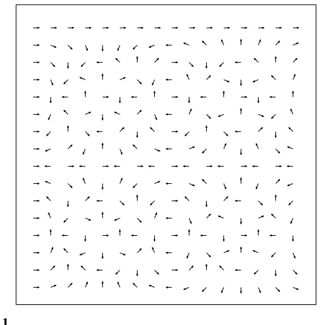
To compare the usefulness of the Markov-1 solution to the KLT, we first look at the autocorrelation of the image. As shown inTable 1.3, the autocorrelation does appear to follow the Markov-1 model of E[x_ix_j] =E[x2_]_ρ|i−j| _with_ρ

(44)

FIGURE 1.15

Details of image before and after 10:1, 20:1, and 40:1 compression. (a) Original, (b) Compressed 10:1, (c) Compressed 20:1, (d) Compressed 40:1. Reproduced by Special Permission ofPlayboymagazine. Copyright ©1972, 2000 by Playboy.

curves are almost identical, the savings in computational resources from having a closed form solution for the Markov-1 case incurs little if any cost in performance.

1.4.5 Medical Imaging

(45)

FIGURE 1.16

Plot of distortion versus bit rate for KLT calculated from both randomly chosen blocks and sequential blocks.

the use of lossless compression in this field; however, such an approach is of limited usefulness due to the theoretical limits on the maximum allowable compression.

(46)

FIGURE 1.17

Second test image, “Goldhill.”

(47)

FIGURE 1.18

Distortion versus bit rate for “Goldhill” image using KLT from both “Goldhill” image and “Lena” image.

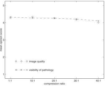
The results of evaluation are summarized inFig. 1.22which shows the plot of the mean opinion score for both scoring criteria. The figure shows that the MOS at the various degrees of compression remains quite close to that of the original. For image quality, the MOS for the original is 4.28 and drops only to 4.01 at 40:1. The MOS for the pathology visibility is 4.33 for the original and 4.10 for the 40:1 compression ratio. Therefore the use of a compression method based on the KLT results in usable images at even relatively high compression.

1.4.6 Color Images

(48)

Table 1.3

Correlation Between First 8 Neighboring Pixels on the Rows

E[x_ix_j] E[x_ix_j]/E[x_i₋1xj]

|i−j| =0 2657

-|i−j| =1 2589 0.9744

|i−j| =2 2472 0.9546

|i−j| =3 2338 0.9460

|i−j| =4 2223 0.9510

|i−j| =5 2111 0.9492

|i−j| =6 2010 0.9524

|i−j| =7 1914 0.9523

in different coordinate spaces [18]. Some, for example HSI, express the components in a form that follows more closely the human perceptions of color qualities such as hue, saturation, and intensity. Others, for example YIQ, attempt to decorrelate the chromatic and intensity information. For the following example, we will explore the use of the decorrelation property of the KLT on the raw RGB data.

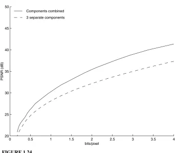
A simple approach to compression would be to treat each of the three RGB com-ponents as separate images. However, this method does not exploit the correlation between the three color values at each pixel. An alternative is to include all three component pixel values within a block. For example, an 8×8 block will contain 192 individual values. The KLT can then decorrelate the component values allowing improved coding.

(49)

FIGURE 1.19

KLT basis images for Markov-1 model,ρ=0.9543.

1.5 Summary

The Karhunen-Loève transform (KLT) is defined as the linear transformation whose basis vectors are the eigenvectors of the covariance matrix of the data. As it diagonal-izes the covariance matrix, it decorrelates the data. The resulting set of coefficients can be encoded with fewer bits for a given distortion than the raw data.

(50)

FIGURE 1.20

Plot of distortion (PSNR) versus bit rate for the KLT from the image covariance matrix and the KLT generated from the Markov-1 model.

the product of all the variances is minimized due to the energy preserving nature of any orthonormal transformation. Since the total differential entropy for the blocks increases with the product of the variances, the KLT minimizes the entropy thereby minimizing the bound on the bit rate.

(51)

FIGURE 1.21

Sample chest radiograph for medical image compression evaluation.

data with more than one component, such as the three RGB components in color images.

(52)

[image:52.612.106.446.126.407.2]

FIGURE 1.22

Mean opinion score across all images and evaluators.

FIGURE 1.23

[image:52.612.111.450.442.676.2]

(53)

[image:53.612.157.499.119.418.2]

FIGURE 1.24

Distortion versus bit rate for “Monarch” image for encoding the RGB compo-nents separately and together.

ratios, yet it is not accounted for in the distortion criteria. A full frame KLT is theoretically possible, but it is only practical for sets of quite small images.

References

[1] Berger, T.,Rate Distortion Theory,Prentice-Hall, Englewood Cliffs, NJ, 1971.

[2] Castleman, K.R.,Digital Image Processing,Prentice-Hall, Englewood Cliffs, NJ, 1996.

(54)

[4] Chen, T., Hua, Y., and Yan, W.-Y., Global convergence of Oja’s subspace algorithm for principal component extraction,IEEE Trans. Neural Networks,

9(1):58–67, 1998.

[5] Clarke, R.J.,Transform Coding of Images,Academic Press, San Diego, CA, 1985.

[6] Clarke, R.J.,Digital Compression of Still Images and Video,Academic Press, San Diego, CA, 1995.

[7] Diamantaras, K.I. and Kung, S.Y.,Principal Component Neural Networks: Theory and Applications,John Wiley & Sons, New York, 1996.

[8] Dony, R.D. and Haykin, S., Optimally adaptive transform coding,IEEE Trans. Image Processing,4(10):1358–1370, 1995.

[9] Dony, R.D., Haykin, S., Coblentz, C., and Nahmias, C., Compression of digital chest radiographs using a mixture of principal components neural network: an evaluation of performance,RadioGraphics,16, 1996.

[10] Gersho, A. and Gray, R.M., Vector Quantization and Signal Compression,

Kluwer Academic Publishers, Norwell, MA, 1992.

[11] GNU Octave,http://www.che.wisc.edu/octave.

[12] Gonzalez, R.C. and Woods, R.E.,Digital Image Processing,Addison-Wesley, Reading, MA, 1993.

[13] Gray, R.M.,Source Coding Theory,Kluwer Academic Publishers, Norwell, MA, 1990.

[14] Haykin, S.,Neural Networks: A Comprehensive Foundation,Macmillan, New York, 1994.

[15] Hotelling, H., Analysis of a complex of statistical variables into principal components,J. Educ. Psychol.,24:417–447, 498–520, 1933.

[16] Jolliffe, I.,Principal Component Analysis,Springer-Verlag, New York, 1986.

[17] Karhunen, K., Über lineare methoden in der wahrscheinlich-keitsrechnung.

Ann. Acad. Sci. Fennicea,Ser. A137, 1947. (Translated by Selin, I. in “On Linear Methods in Probability Theory,” Doc. T-131, The RAND Corp., Santa Monica, CA, 1960.)

[18] Levkowitz, H.,Color Theory and Modeling for Computer Graphics, Visual-ization, and Multimedia Applications,Kluwer Academic Publishers, Norwell, MA, 1997.

[19] Loève, M., Fonctions Aléatoires de second order, In Lévy, P., Ed.,Processus Stochastiques et Movement Brownien,Hermann, Paris, 1948.

[20] MathWorks,http://www.mathworks.com.

(55)

[22] Netlib Repository,http://www.netlib.org/lapack.

[23] Netlib Repository,http://www.netlib.org/linpack.

[24] Netravali, A.N. and Haskell, B.G.,Digital Pictures: Representation and Com-pression,Plenum Press, New York, 1988.

[25] Oja, E., A simplified neuron model as a principal component analyzer,J. Math. Biology,15:267–273, 1982.

[26] Oja, E., Neural networks, principal components, and subspaces,Int. J. Neural Systems,1(1):61–68, 1989.

[27] Oja, E. and Karhunen, J., On stochastic approximation of the eigenvectors and eigenvalues of the expectation of a random matrix,J. Math. Analysis and Applications,106:69–84, 1985.

[28] Press, W.H., Flannery, B.P., Teukolsky, S.A., and Vetterling, W.T.,Numerical Recipes in C: The Art of Scientific Computing,Cambridge University Press, Cambridge, UK, 1988.

[29] Rao, K.R. and Yip, P., Discrete Cosine Transform: Algorithms, Advantages, Applications,Academic Press, New York, 1990.

[30] Ray, W. and Driver, R.M., Further decomposition of the Karhunen-Loève series representation of a stationary random process,IEEE Trans. Information Theory,IT-16:663–668, 1970.

[31] Research Systems,http://www.rsinc.com.

[32] Rosenfeld, A. and Kak, A.C.,Digital Picture Processing,Vol. I & II, 2nd ed., Academic Press, San Diego, CA, 1982.

[33] Sanger, T.D., Optimal unsupervised learning in a single-layer linear feedfor-ward neural network,Neural Networks,2:459–473, 1989.

[34] Shannon, C.E., A mathematical theory of communication, The Bell System Technical J.,27(3):379–423, 623–656, 1948.

[35] Solo, V. and Kong, X., Performance analysis of adaptive eigenanalysis algo-rithms,IEEE Trans. Signal Processing,46(3):636–645, 1998.

[36] Wallace, G.K., The JPEG still image compression standard,Communications of the ACM,34(4):30–44, 1991.

(56)

Ivan W. Selesnick et al. "The Discrete Fourier Transform"

The Transform and Data Compression Handbook

Ed. K. R. Rao et al.

(57)

Chapter 2 The Discrete Fourier Transform

Ivan W. Selesnick

Polytechnic University

Gerald Schuller

Bell Labs

2.1 Introduction

The discrete Fourier transform (DFT) is a fundamental transform in digital signal processing, with applications in frequency analysis, fast convolution, image process-ing, etc. Moreover, fast algorithms exist that make it possible to compute the DFT very efficiently. The algorithms for the efficient computation of the DFT are collectively called fast Fourier transforms (FFTs). The historic paper by Cooley and Tukey [15] made well known an FFT of complexityNlog2N, whereNis the length of the data

vector. A sequence of early papers [3, 11, 13, 14, 15] still serves as a good reference for the DFT and FFT. In addition to texts on digital signal processing, a number of books devote special attention to the DFT and FFT [4, 7, 10, 20, 28, 33, 36, 39, 48]. The importance of Fourier analysis in general is put forth very well by Leon Co-hen [12]:

. . . Bunsen and Kirchhoff, observed (around 1865) that light spectra can be used for recognition, detection, and classification of substances because they are unique to each substance.

This idea, along with its extension to other waveforms and the invention of the tools needed to carry out spectral decomposition, certainly ranks as one of the most important discoveries in the history of mankind.

Thekth DFT coefficient of a lengthN sequence{x(n)}is defined as

X(k)=

N−1

n=0

(58)

where

WN =e−j2π/N =cos

2π

N

−j sin

2π

N

is the principalN-th root of unity. BecauseW_Nnk as a function ofkhas a period of

N, the DFT coefficients{X(k)}are periodic with periodN whenkis taken outside the rangek =0, . . . , N−1. The original sequence{x(n)}can be retrieved by the inverse discrete Fourier transform (IDFT)

x(n)= 1 N

N−1

k=0

X(k) W_N−kn, n=0, . . . , N−1.

The inverse DFT can be verified by using a simple observation regarding the principal

N-th root of unityW_N. Namely,

N−1

n=0 Wnk

N =N·δ(k), k=0, . . . , N−1,

whereδ(k)is the Kronecker delta function defined as

δ(n)=

1 n=0

0 n=0.

For example, withN =5 andk=0, the sum gives

1+1+1+1+1=5.

Fork=1, the sum gives

1+W5+W52+W 3 5 +W

4 5 =0

THE TRANSFORM AND DATA COMPRESSION HANDBOOK K R RAO pdf

The Transform and Data Compression Handbook

Ed. K. R. Rao and P.C. Yip.

THE

TRANSFORM

AND DATA

COMPRESSION

THE ELECTRICAL ENGINEERING

AND SIGNAL PROCESSING SERIES

Edited by Alexander Poularikas and Richard C. Dorf

Handbook of Antennas in Wireless Communications

Lal Chand Godara

Propagation Data Handbook for Wireless Communications

Robert Crane

The Digital Color Imaging Handbook

Guarav Sharma

Handbook of Neural Network Signal Processing

Yu Hen Hu and Jeng-Neng Hwang

Handbook of Multisensor Data Fusion

David Hall

The Advanced Signal Processing Handbook:

Theory and Implementation for Radar, Sonar,

and Medical Imaging Real Time Systems

Stergios Stergiopoulos

The Transform and Data Compression Handbook

K.R. Rao and P.C. Yip

The Encyclopedia of Signal Processing

Alexander Poularikas

THE

TRANSFORM

AND DATA

COMPRESSION

HANDBOOK

Edited by

K.R. RAO

University of Texas at Arlington

AND

Preface

Outline of Chapters

Acknowledgements

List of Acronyms

Contributors

Contents

The Transform and Data Compression Handbook

Ed. K. R. Rao and P.C. Yip.

Chapter 1

Karhunen-Loève Transform

1.1

Introduction

1.2

Data Decorrelation

--

-

-

1.2.1

Calculation of the KLT

1.3

Performance of Transforms

1.3.1

Information Theory

1.3.2

Quantization

1.3.3

Truncation Error

Table 1.1

1.3.4

Block Size

1.4

Examples

1.4.1

Calculation of KLT

--

-

-

1.4.2

Quantization and Encoding

--

-

--

-