Sufficient Dimension Reduction

(1)

Jingyue Lu

Primary Supervisor: Professor Alan Welsh

July 2017

A thesis submitted for the degree of Master of Philosophy

of The Australian National University

(2)

(3)

I, Jingyue Lu, declare that this thesis titled, ‘Sufficient Dimension Reduction’ and the

work presented in it are my own. I confirm that:

This work was done wholly or mainly while in candidature for a research degree at

this University.

Where I have consulted the published work of others, this is always clearly attributed.

Where I have quoted from the work of others, the source is always given. With the

exception of such quotations, this thesis is entirely my own work.

I have acknowledged all main sources of help.

Signed:

Date:

(4)

(5)

First and foremost, I would like to express my sincere gratitude to my supervisor, Professor

Alan Welsh, for his valuable comments, remarks and engagement through the learning

process of this master thesis. Alan has not only introduced me to the topic of the thesis,

but also helped me gain a deeper understanding of statistics through many insightful

conversations.

On a more personal level, I am thankful to my friend Xiaoyang Xu, for all the times he has

lifted my spirit with his healthy cooking and shared laughter. Last but not least, I want

to thank my parents for encouraging me in all my pursuits and inspiring me to follow my

dreams.

This research is supported by Australian Government Research Training Program

Fee-Offset Scholarship.

(6)

(7)

In regression analysis, it is difficult to uncover the dependence relationship between a

re-sponse variable and a covariate vector when the dimension of the covariate vector is high.

To reduce the dimension of the covariate vector, one approach is sufficient dimension

re-duction. Sufficient dimension reduction is based on the assumption that the response

variable relates to only a few linear combinations of the covariate vector. Thus, by

re-placing the covariate vector with these linear combinations, sufficient dimension reduction

achieves dimension reduction. The goal of sufficient dimension reduction is to estimate

the space spanned by these linear combinations of the covariate vector. We denote this

space by S.

In this thesis, we give an introductory review on three important sufficient dimension

reduction methods. They are Sliced Inverse Regression (SIR), Sliced Average Variance

Estimate (SAVE) and Principle Hessian Directions (pHd). Li proposed SIR in 1991. SIR

is a method that exploits the simplicity of the inverse regression. Given the univariate

response variable and the high dimensional covariate, it is much easier to regress the

covariate against the response variable than the other way around. Motivated by a theorem

that connects forward regression and inverse regression, SIR estimates S using inverse

regression lines. Since SIR uses first moments only, it fails when there exists symmetry

dependence between the response variable and the covariate. To make up for this defect,

Cook proposed SAVE in a comment on SIR in 1991. SAVE follows the general lines of

SIR but uses second moments as well as first moments to estimate S. pHd is also a second

moment method. Li developed pHd in 1992 based on the observation that the eigenvectors

for the Hessian matrices of the regression function are closely related to the basis vectors

of S. Therefore pHd provides an estimate of S by using these eigenvectors.

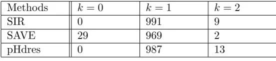
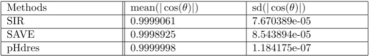
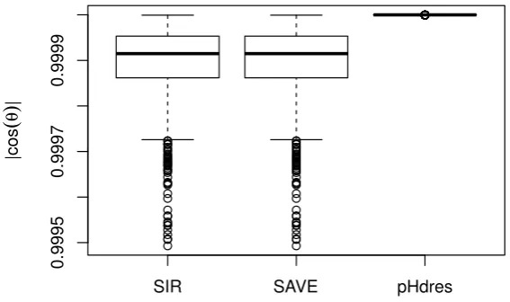
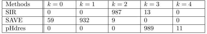
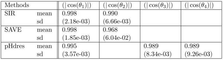
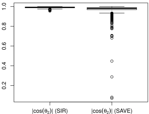
To compare these methods, a simulation study is presented at the end. From the simulation

results, SIR is the most efficient method and SAVE is the most time consuming method.

Since SIR fails when symmetry dependence exists, we recommend pHd when symmetry

dependence presents and SIR in other cases.

(8)

(9)

Declaration of Authorship iii

Acknowledgements v

Abstract vii

1 Introduction 1

1.1 Problem set up . . . 1

1.2 Project outline . . . 2

2 Elliptically contoured distributions 5 2.1 Definition and Characterisation . . . 5

2.2 Basic properties. . . 12

2.2.1 Density functions . . . 13

2.2.2 Moments . . . 15

2.2.3 Marginal distributions . . . 18

2.2.4 Conditional distribution . . . 19

3 Central subspaces 27 3.1 Conditional Independence . . . 27

3.2 Problem set up . . . 28

3.3 Dimension reduction subspaces . . . 30

3.4 Central subspaces. . . 32

3.5 Existence of the central subspace . . . 33

4 SIR and SAVE 41 4.1 Sliced Inverse Regression. . . 41

4.1.1 Inverse Regression Subspace. . . 42

4.1.2 Finding a connection betweenSy|x andSE(x|y) . . . 43

4.1.3 EstimatingS_E(_z|y) . . . 48

4.1.4 SIR Algorithm . . . 49

4.1.5 A method for choosing the dimensionS{Var[E(z|y˜)]} . . . 51

4.1.6 Comments on SIR . . . 58

4.1.6.1 Comment One: e.d.r. directions . . . 58

4.1.6.2 Comment Two: slices . . . 59

4.1.6.3 Comment Three: limitations of SIR . . . 59

4.2 SAVE . . . 60

4.2.1 A method for choosing the dimension ofS(Σsave) . . . 63

4.3 Conclusion . . . 67

(10)

5 pHd 69

5.1 Principal Hessian Directions . . . 69

5.1.1 Response based pHd . . . 70

5.1.2 Residual based pHd . . . 74

5.1.3 EstimatingSe|z . . . 79

5.1.3.1 Cook’s approach . . . 80

5.1.4 pHdres algorithm . . . 82

5.1.5 A method for choosing the dimension ofSezz . . . 83

6 Simulations 89 6.1 Example One: . . . 89

6.2 Example Two: . . . 92

6.3 Example Three: . . . 98

(11)

Introduction

With technological advances, datasets have grown in both size and complexity. One

con-sequence of increasing amounts of data is that we often need to relate a response variable

to a potentially large number of possible covariates. The high dimension of the

covari-ate space makes it difficult to uncover this relationship. To reduce the dimension of the

covariate space, two major approaches are developed based on different assumptions.

The first approach is variable selection. Variable selection is used when researchers believe

that among all available predictors, only a few have explanatory effect. Thus, variable

se-lection reduces the number of covariates by identifying and removing the covariates that

have non explanatory effect. The second approach is sufficient dimension reduction.

Suffi-cient dimension reduction, on the other hand, assumes that each covariate has explanatory

effect, but the explantory effect is only represented through a few linear combinations of

covariates. Therefore, sufficient dimension reduction aims to find these linear

combina-tions. By replacing the collection of covariates with these linear combinations, sufficient

dimension reduction achieve dimension reduction of the covariate space.

In this thesis, we focus on the second approach: sufficient dimension reduction.

1.1 Problem set up

Throughout the thesis, we denote the response variable asy∈Rand the covariate vector

asx= (x1, . . . , xp)T ∈Rp.

(12)

Given the assumption of sufficient dimension reduction, the main problem of sufficient

dimension reduction can be described by the model

y =f(β₁Tx, β₂Tx, . . . , βT_kx, ), (1.1)

whereβ’s are unknown column vectors of the matrix Φ := (β1, β2, . . . , βk),is independent

of x, andf is an arbitrary unknown function on Rk+1. If we can find Φ, we can replace

p dimensional covariatex withβ₁Tx, βT₂x, . . . , β_kTx. Sincekis typically much smaller than

p, we hence achieve dimension reduction.

However, Φ is not identifiable. LetS(A) be the space spanned by columns of an arbitrary matrix A. We observe that if (1.1) holds, then it also holds when we replace Φ with any

matrix A such thatS(A) = S(Φ). Therefore, it is appropriate to identify S(Φ) instead. We call a subspaceS(Φ) satisfying (1.1) adimension reduction subspace (DRS) (Li,1991). Because S(Ip) is by definition a DRS, DRS always exists and is not always unique.

To achieve maximum dimension reduction, we are interested in finding a minimum DRS.

A minimum DRS Smin is a DRS such that dim(Smin)≤dim(Sdrs) for all DRSs Sdrs. As

we will see in Chapter 3, a minimum dimension reduction subspace may not be unique,

leading to complications at later stages. In order to deal with this issue, we adopt Cook’s

idea (Cook, 2009) and introduce the concept of central dimension reduction subspaces

(or central subspaces), denoted as S_y|x. A central subspace, when exists, is the unique

minimum dimension reduction subspace. Since central subspaces exist under various

rea-sonable conditions (Cook, 1994a, 1996), we restrict ourselves to the class of regressions

for which the central subspace exist to ensure the uniqueness of the minimum dimension

reduction subspace. Thus, we conclude the goal of sufficient dimension reduction is to find

the central subspace of a problem of interest. More details are provided in Chapter 3.

1.2 Project outline

The purpose of this thesis is to provide readers with an introductory review on three

sufficient dimension reduction (SDR) methods, which are Sliced Inverse Regression (SIR)

(Li,1991), Sliced Average Variance Estimation (SAVE) (Cook and Weisberg,1991), and

Principal Hessian Directions (pHd) (Li,1992;Cook,1998). In particular, we want to see

how we can use these methods to at least partially recover the central subspace Sy|x to

(13)

The rest of the thesis is organized in the following way. Chapter 2 is a preparation chapter.

It gives a short introduction to elliptically contoured distributions and their properties.

Since elliptically contoured distributions are closely related to the prerequisites of many

SDR methods, studying them should help us gain a better understanding of SDR methods

later.

Chapter 3-6 are about SDR methods. Chapter 3 sets up a theoretical framework for

our studies of SDR methods. It studies central subspaces in detail by addressing the

key questions: What are central subspaces? Why do we need central subspaces? And

when do central subspaces exist? Discussions of the SDR methods SIR, SAVE and pHd

are contained in Chapter 4 and Chapter 5. For each method, we not only examine the

theoretical foundations, but also provide a step by step algorithm for estimating the central

subspaceSy|x. Since each method has its advantages and disadvantages, a simulation study

for testing and comparing the SDR methods SIR, SAVE and pHd is presented in the final

(14)

(15)

Elliptically contoured distributions

Before we delve into specific sufficient dimension reduction (SDR) methods, we first

in-troduce elliptically contoured distributions, which, as we will show in later chapters, are

closely related to the key prerequisites required for most SDR methods to work.

Ellipti-cally contoured distributions are a natural generalization of Gaussian distributions. When

the covariate has an elliptically contoured distribution, many SDR methods are able to

exploit the nice properties of elliptically contoured distributions inherited from Gaussian

distributions to attain neat and compact results. In this chapter, we examine the basic

but essential properties of elliptically contoured distributions.

2.1 Definition and Characterisation

Despite being a generalization of Gaussian distributions, elliptically contoured

distribu-tions are generally treated as an extension of spherical distribudistribu-tions. In this section, we

adopt this way of classifying them and start by introducing spherical distributions

follow-ing the ideas ofKelker (1970) and Frahm(2004).

Definition 2.1(Spherical distribution). LetXbe ap-dimensional random vector. Xhas a p-dimensional spherical distribution if and only if, for all Rp×p orthonormal matrices Γ,

X and ΓX have the same distribution such thatX =dΓX.

Spherical distributions are also referred to as radial distributions. To better understand

this definition, we first note that when a random vector X satisfies X =d ΓX for any p

(16)

byporthonormal matrix Γ,X is rotationally symmetric. As a result, the above definition can be equally stated as follows.

Let X be a p-dimensional random vector. X has ap-dimensional spherical distribution if and only if it is rotationally symmetric.

Recall that if we let U(p) be a p-dimensional random vector that is uniformly distributed on the unit sphere

Sp−1:={x∈Rp :kxk2= 1},

and assume R is a nonnegative random variable independent of U(p), then every p -dimensional random vector Y with the form ofY :=RU is rotationally symmetric. Since spherical distributions and rotationally symmetric distributions are identical, Y is spher-ically distributed. Hence, we have found an explicit form that ensures a random vector

follows a spherical distribution. A question arises naturally: can any spherically

dis-tributed random vectorX be written in the form of RU? If this is the case, the analysis of spherical distributions can be conducted in a straightforward manner, as we can work

withU and R directly instead.

In order to answer this question, we consider a spherically distributedp-dimensional ran-dom vector X. Because X is, by definition, rotationally symmetric, for any t∈ _Rp_{, the}

equality

cos(](t, X)) =dcos(](v, U(p))) =dvTU(p) (2.1)

holds for every v∈Sp−1 and random vector U(p) uniformly distributed on Sp−1 (Frahm,

2004). Here, ](t, X) measures the angle between p-dimensional vector t and the random vectorX and we have used the fact thattTX =ktk₂· kXk₂·cos(](t, X)). As a result of this equality, the characteristic function of cos(_](t, X)) satisfies

t7−→ϕ_cos(](t,X))(s) =ϕ_vT_U(p)(s)

:= E{exp(isvTU(p))}= E{exp(i(sv)TU(p))}

=ϕ_U(p)(sv)

(2.2)

wherev∈Sp−1 is arbitrary andϕ_U(p) is the characteristic function ofU(p). This

(17)

as follows

t7−→ϕX(t) = E{exp(itTX)}= E{exp(i· kXk2· ktk2·cos(](t, X)))}.

Then applying the law of total expectations to derive that

t7−→ϕX(t) = EX[E{exp(i· kXk2· ktk2·cos(](t, X)))| kXk2=r}]

=

Z ∞

0

E{exp(i·rktk₂cos(](t, X)))}dFkXk2(r)

=

Z ∞

0

ϕ_cos(](t,X))(rktk2)dFkXk2(r),

whereFkXk2 is the cumulative distribution function (c.d.f) ofkXk2. Then by the

relation-ship (2.2), we have

t7−→ϕX(t) = Z ∞

0

ϕ_cos(](t,X))(rktk₂)dFkXk2(r)

=

Z ∞

0

ϕ_U(p)(rktk2·

t

ktk₂)dFkXk2(r).

Here, we have replaced the v in (2.2) witht/ktk2∈Sp−1. Finally, we obtain

t7−→ϕX(t) = Z ∞

0

ϕ_U(p)(rktk2·

t

ktk₂)dFkXk2(r)

=

Z ∞

0

ϕ_U(p)(rt)dF_k_X_k₂(r)

=

Z ∞

0

ϕ_rU(p)(t)dFkXk2(r)

for anyr ≥0. We note that the last line of above equation can be viewed as the charac-teristic function of the random vector RU(p), where R is a nonnegative random variable independent ofU(p)and having the same distribution askXk2. We thus have successfully

shown that any spherical distributedp-dimensional random vectorX has the representa-tion X=dRU(p). Once pis given, U(p) is fully determined and the spherical distribution

ofX is completely decided by the non-negative random variable R. Therefore,Ris often called “generating random variable” or “generating variate” of X (Frahm,2004).

Remark 2.2. From the definition of spherical distributions, we see that a spherical

distribu-tion is invariant under rotadistribu-tion. This implies that spherical distribudistribu-tions are distribudistribu-tions

that are centered about zero. Thus, when the expectation of a spherical distribution exists,

the expectation has be to 0. We can prove this statement by using either the definition or

(18)

Assume a p-dimensional random vector X is spherically distributed and its mean exists. We first show E(X) = 0 by definition. Let Γ1 6= Γ2 be orthonormal matrices. SinceX =d

Γ1X =dΓ2X, E(X) = E(Γ1X) = E(Γ2X). That is E((Γ1−Γ2)X) = (Γ1−Γ2)E(X) = 0.

Because we know that (Γ1−Γ2)6= 0, we conclude that E(X) = 0. On the other hand, we

have shown that X has the representation X =d RU(p). Since R is independent of U(p)

and E(U(p)) = 0, we also derive that E(X) = E(R)·E(U(p)) = 0.

Remark 2.3. Given the fact that every spherical distribution has the representationX =d

RU(p), we can easily deduce the generating variable for standard normal distributions. Assume X ∼ Np(0, Ip) and has the representation X =d RU(p) as defined above. Then

we have

χ2_p =dXTX=R2U(p)TU(p)=a.s.R2.

It follows that the generating variable of a standard normal distribution isqχ2

p, the square

root of a random variable with a chi-squared distribution with pdegrees of freedom.

In addition to the generating random variable R, we can also find the characteristic generator function of a spherically distributed random vectorX by closely examining the characteristic function ϕX and exploring theRU(p) representation. The key observation

to make is that, for the characteristic functionϕ_U(p) ofU(p), we can always find a function

φ_U(p) such that ϕ_U(p)(sv) = φ_U(p)(s2) for every s ∈ R. As mentioned in (2.2), we note

that, given that the point v is arbitrary, ϕ_U(p)(sv) only depends on s. In addition, since

ϕ_U(p)((−s)v) =ϕ_U(p)(s(−v)), ϕ_U(p)(sv) is independent of the sign of sand hence can be

treated as a function of s2. We thus obtain

t7−→ϕX(t) = Z ∞

0

ϕ_rU(p)(t)dFR(r)

=

Z ∞

0

ϕ_U(p)(rt)dFR(r)

=

Z ∞

0

ϕ_U(p)(rktk₂·

t

ktk₂)dFR(r)

=

Z ∞

0

φ_U(p)(r2ktk2₂)dFR(r).

(2.3)

Consequently, ϕX can be equally represented through

s7−→φX(s) := Z ∞

0

φ_U(p)(r2s)dFR(r) s≥0 (2.4)

with

(19)

Moreover, we observe that if ap-dimensional random vectorX has characteristic function

ϕ(t) satisfying ϕ(t) = φ(tTt) for some function φ, then X is spherically distributed by definition, as the characteristic function implies thatX=dΓXfor all orthonormal matrices

Γ∈_Rp×p_.

Combining previous results, we conclude a random vectorX belongs to the class of spheri-cal distributions if and only if the equality (2.5) holds. As a result,φX is generally referred

to as “characteristic generator” ofX(Schmidt,2002). We point out that the characteristic generator captures all the information contained inR.

Remark 2.4. It is easy to deduce that the characteristic generator of a random vector X

with standard normal distribution isφX(s) = exp(−s/2) given thatϕX(t) = exp(−tTt/2)

and φX(tTt) =ϕX(t).

We now extend our discussions to elliptically contoured distributions. As we mentioned

at the beginning, elliptical contoured distributions are a generalization of spherical

dis-tributions. To be more specific, we will see shortly that every affine transformation of

a spherically distributed random vector follows an elliptically contoured distribution and

the converse is also true. Before we give proofs for these statements, we first give a formal

definition of elliptically contoured distributions.

Definition 2.5 (Elliptically contoured distributions). LetX be ap-dimensional random vector. X is said to be “elliptically distributed” or just “elliptical” if and only if there exits a constant vector µ∈ _Rp_{, a symmetric positive semidefinite matrix Σ}_∈

Rp×p, and

a function φ :R+ → R such that the characteristic function ϕX−µ(t) of X−µ satisfies

ϕX−µ(t) = φ(tTΣt). We write X ∼ ECp(µ,Σ, φ), where EC is short for elliptically

contoured.

Thus, to show that every affinely transformed spherical random vector is elliptically

dis-tributed, it is sufficient to find the characteristic function of the transformed random vector

and check the existence of the functionφ, satisfyingϕX−µ(t) =φ(tTΣt). Based upon this

idea, we have the following proposition.

Proposition 2.6. Let X be a k-dimensional spherically distributed random vector with characteristic generator φX. Also assume Λ∈Rp×k is an arbitrary matrix and µ∈Rp is an arbitrary vector. Then Y :=µ+ ΛX has the characteristic function

(20)

where Σ := ΛΛT_{. Consequently,} _Y _{is elliptically distributed.}

Proof. We prove this proposition by directly computing the characteristic function of Y. We have

t7−→ϕY(t) = E(exp(itT(µ+ ΛX))) = exp(itTµ)·ϕX(ΛTt)

= exp(itTµ)·φX((ΛTt)T(ΛTt)) = exp(itTµ)·φX(tTΣt).

It follows

t7−→ϕY−µ(t) =ϕX(ΛTt) =φX(tTΣt),

soY has an elliptically contoured distribution by definition.

Remark 2.7. In fact, this proposition partly motivates the definition of elliptically

toured distribution above and, to some extent, serves as a basis to define elliptically

con-toured distributions with a focus on the characteristic generators. Further, we emphasize

thatY need not necessarily have the same dimension asX.

For the other direction, to show that every elliptically contoured distribution is an affinely

transformed spherical distribution, we use the stochastic representation theorem. We recall

that every spherically distributed random vector X has the representation X =d RU(k).

The stochastic representation theorem proves the statement by showing that, under certain

conditions, every Y ∼ECp(µ,Σ, φ) has the stochastic representation Y =d µ+RΛU(k),

which is just the affine transformation of the spherically distributed random vectorRU(k). Theorem 2.8 (Stochastic representation theorem). Let Y be p-dimensional random vec-tor. Then Y ∼ECp(µ,Σ, φ) with rank(Σ) =kif and only if

Y =dµ+RΛU(k)

whereRis a nonnegative random variable,U(k) _is_k_{-dimensional random vector uniformly} distributed on Sk−1 that is independent of R, µ∈_Rp _and_Λ_∈

Rp×k with rank(Λ) =k.

Proof. We have proved the “if” direction in the proposition above. To show the “only

if” direction, we note that every rank k symmetric positive semidefinite matrix Σ can be decomposed as Σ = ΛΛT where Λ∈_Rp×k_{. Then, define the random vector}

(21)

where Λ† := (ΛT_Λ)−1_ΛT _{is the Moore-Penrose pseudoinverse of Λ. Calculating the}

char-acteristic function of X, we obtain

t7−→ϕX(t) =ϕY−µ((Λ†)Tt) =φ(tTΛ†Σ(Λ†)Tt)

=φ(tT(ΛTΛ)−1ΛT(ΛΛT)Λ(ΛTΛ)−1t) =φ(tTt), t∈Rk.

(2.6)

This implies thatXis spherically distributed with the characteristic generatorφ(tTt) and can be represented asX=dRU(k). HenceY =µ+ΛX=dµ+RΛU(k)∼ECp(µ,Σ, φ).

We make some important comments about the stochastic representations of elliptically

contoured distributions.

• Firstly, although each elliptically contoured distributed random vector can be

formu-lated in stochastic representation, it should be emphasized that this representation

is not unique. To be more specific, a stronger statement has been proved by

Cam-banis et al. (1981). It states that, given X is nondegenerate, if X ∼ECp(µ,Σ, φ)

andX ∼ECp(µ0,Σ0, φ0), then there exists a constantc >0 such that Σ0=cΣ and

φ0(·) =φ(c−1·) whileµ=µ0. It is possible for Σ andφ to be different from Σ0 and

φ0 but the differences are up to a constant.

• Secondly, we note that an elliptically distributed random vector X ∼ECp(0, Ip, φ)

withµ= 0 and Σ =Ipis spherically distributed asX= 0+RIpU(p)=RU(p). Using

the same line of reasoning, we also find that affine transformations of elliptically

dis-tributed random vectors are also elliptically disdis-tributed. ConsiderY ∼ECp(µ,Σ, φ)

with stochastic representation Y =d µ+RΛU(k) where Λ ∈ Rp×k and ΛΛT = Σ.

Further, let α ∈Rm and A ∈Rm×p. Assume the random vector W is transformed

from Y by

W =α+AY.

Then we obtain

W =dα+A(µ+RΛU(k)) = (α+Aµ) +RAΛU(k),

which implies W ∼ ECm(α+Aµ, AΣAT, φ). That is, W is elliptically distributed

withϕW−(α+Aµ)(t) =φY(tTAΣATt). In conclusion, the class of elliptical contoured

(22)

• Finally, the stochastic representation of an elliptically contoured distribution is

gen-erally preferred to its characteristic representation. Not only does the stochastic

representation give a straightforward geometric interpretation of an elliptically

dis-tributed random vector X (µ determines the location of X, R specifies the shape, especially the tailedness of the distribution while Λ andU(k) together produces den-sity surface), but also the explicit representations facilitate the simulation process

of X (Frahm,2004).

Remark 2.9. Multivariate normal distributions are a special case of elliptically contoured

distributions. To see this, let X∼Np(µ,Σ) be a random vector with multivariate normal

distribution, where µ ∈ Rp and Σ ∈ Rp×p is positive definite with the decomposition

Σ = ΛΛT with Λ∈_Rp×k_{. Then from remark}_2.3_{, we can derive that}

X=dµ+ q

χ2 kΛU

(k)

and hence X is elliptically distributed. In addition, from Remark 2.4, we have the char-acteristic functionϕX−µ of X−µsatisfiest7−→ϕX−µ(t) = exp(tTΣt).

So far, we have introduced elliptically contoured distributions as an extension of spherical

distributions. We have also shown that elliptically contoured distributions have stochastic

representations, that is they can be represented as an affine transformation of a spherical

distributionRU(k). With this explicit expression for elliptically contoured random vectors, we can easily develop the basic properties of this class of distributions, covered in the

following section.

2.2 Basic properties

In this section, we study the density functions, marginal distribution and conditional

distributions of elliptically contoured distributions. The main focus will be on the

condi-tional distributions as their properties are the key for most sufficient dimension reduction

(23)

2.2.1 Density functions

Adopting the same analysing procedure as that used above, to find the density function of

the elliptically contoured distributions, we first derive the density function of the spherical

distributions.

Theorem 2.10 (Spherical distributions). Let X be a p-dimensional random vector with stochastic representationX =dRU(p) where the c.d.f ofR is absolutely continuous. Then the c.d.f of X is given by

x7−→fX(x) =

Γ(p₂) 2πp/2 · kxk

−(p−1)

2 ·fR(kxk2), x∈Rp\ {0},

where fR is the p.d.f ofR.

Proof. To start, we recall that the density function of a p-dimensional random vector uniformly distributed on the unit hypersphere Sp−1 is Γ(

p 2)

2πp/2 and that U

(p) _and _R _are

independent. Thus, given that the c.d.f of R is absolutely continuous, we have that the density function of the pair (r, u) is

(r, u)7−→f₍_R_,U(p)₎(r, u) =

Γ(p₂)

2πp/2 ·fR(r), r >0, u∈S p−1_.

In order to find the density function of X =d RU(p), we define the transformation h :

(0,∞)×Sp−1 →_Rp_{\ {}₀_} _by _h₍_{r, u}_{) =}_ru_{. Clearly,} _h _{is injective. We thus have the p.d.f}

of X as

x7−→fX(x) =fR,U(p)(h−1(x))· |J_h|−1, x∈_Rp\ {0}, (2.7)

where Jh is the Jacobian determinant of ∂ru/∂(r, u)T. Since for any u∈Sp−1,kuk= 1,

it follows thatkruk=r. As a result,h−1₍_x_{) = (}_k_x_k

2, x/kxk2). When the Jacobian Jh is

considered, direct calculation gives us

|Jh|=det( 



1 0

0 rIp−1 

) =rp

−1 ₌_k_x_kp−1

2 .

Here we have used the fact that∂ru/∂r has unit length and is orthogonal to∂ru/∂uT on

(24)

Substituting the above results into (2.7), we have derived the p.d.f. ofX as:

x7−→fX(x) =fR,U(p)(kxk2, x/kxk2)· kxkp₂−1

= Γ(

p 2)

2πp/2 · kxk −(p−1)

2 ·fR(kxk2), x∈Rp\ {0}.

(2.8)

Remark 2.11. We can apply this theorem to derive the density function of a standard

normally distributed random vector X∼Np(0, Id). Given that the p.d.f ofχ2p is

t7−→f(t) = t

p

2−1·exp(−t 2)

2p/2_·_Γ(p 2)

, t≥0,

and R=qχ2

p, we get

t7−→fR(t) = 2t·f(t2).

Then it follows from the above theorem, the density function of X is

x7−→fX(x) =

Γ(p₂) 2πp/2 · kxk

−(p−1)

2 ·2kxk2·f(x T_x₎

= Γ(

p 2)

2πp/2 · kxk −(p−1)

2 ·2kxk2·

(xTx)p2−1·exp(−x

T_x

2 )

2p/2_·_Γ(p 2)

= 1

(2π)p/2 ·exp(−

xTx

2 ).

The result for spherical distributions can be easily extended to elliptically contoured

dis-tributions with a positive definite Σ.

Theorem 2.12 (Elliptically contoured distributions). LetX ∼EC(µ,Σ, φ) whereµ∈_Rp andΣ∈_Rp×p_{is symmetric positive definite. Equivalently, we can write}_X_{in its stochastic} representation X =dµ+RΛU(p) where ΛΛT = Σ and Λ∈Rp×p. Assume the c.d.f of R is absolutely continuous, then the p.d.f of X is given by

x7−→fX(x) =|det(Σ)|−1/2·gR((x−µ)TΣ−1(x−µ)), x−µ∈SΛ\ {0}

where

t7−→gR(t) :=

Γ(p₂) 2πp/2 ·

√

t−(p−1)·fR(

√

(25)

Proof. From the theorem above, the density function ofY :=RU(p) _is

y7−→fY(y) =

Γ(p₂) 2πp/2 · kyk

−(p−1)

2 ·fR(kyk2).

To derive the density function ofX, we introduce the transformationh:Rp\{0} →SΛ\{0}

with h(y) = Λy. We note that h(y) =x−µ and h is injective as Λ is invertible , so we have

x7−→fX(x) =fY(h−1(x−µ))· |Jh|−1.

Since h−1(x−µ) = Λ−1(x−µ) and ∂(µ+ Λy)/∂yT = Λ implies that|Jh|=|det(Λ)|, we

hence conclude the p.d.f of X is: for x−µ∈SΛ\ {0}

x7−→fX(x) =fY(Λ−1(x−µ))· |det(Λ)|−1

=|det(Λ)|−1· Γ(

p 2)

2πp/2 · kΛ

−1₍_x₋_µ₎_k−(p−1)

2 ·fR(kΛ

−1₍_x₋_µ₎_k 2).

(2.9)

Finally as

|det(Λ)|=|det(Σ)|1/2

(Λ−1)TΛ−1 = (ΛT)−1Λ−1 = (ΛΛT)−1= Σ−1,

we can replace|det(Λ)|−1 _with_|_det_(Σ)_|−1/2 _and_k_Λ−1₍_x₋_µ₎_k 2 with

p

(x−µ)T_Σ−1₍_x₋_µ₎

respectively. The desired result is thus obtained.

From the theorem above, we see that when elliptically contoured distributions have a

positive definite Σ, their density functions can be expressed in terms of the density function

of the generating random variableR.

2.2.2 Moments

We can also use stochastic representations to find the mean and covariance of a p -dimensional elliptical random vectorX. Assume theX has the stochastic representation

X =dµ+RΛU(k) withR,U(k) defined as above and Λ∈Rp×k, µ∈Rk. Then the mean

of X is

E(X) = E(µ+RΛU(k)) =µ+ ΛE(R)·E(U(k)),

(26)

When the covariance of X is considered, we compute

Cov(X) = E((RΛU(k))(RΛU(k))T) = E(R2)·ΛE(U(k)U(k)T)ΛT. (2.10)

Here we require that E(R2₎ _< _∞_{. To derive the explicit formula for Cov(}_X_{), we thus}

need to obtain the explicit expressions for E(R2_{) and E(}_U(k)_U(k)T_{) respectively.}

We start with the simpler calculation: E(U(k)U(k)T). Since the distribution of U(k) is known, E(U(k)U(k)T) is a fixed number. Thus, by letting R be

q

χ2

k distributed, we can

derive its value by using familiar facts of normal and chi-square distributions. We recall

that from previous remarks, we have concluded that

q

χ2 kU

(k)_∼_N

k(0, Ik). It follows that

Ik= E(( q

χ2 kU

(k)₎₍q_χ2 kU

(k)₎T_{) = E(}_χ2

k)·E(U(k)U(k)T) =k·E(U(k)U(k)T),

which impliesE(U(k)_U(k)T_{) =}_I k/k.

To obtain the value forE(R2_{), we need the following theorem proved by}_{Cambanis et al.}

(1981).

Theorem 2.13. Let X ∼ ECp(µ,Σ, φ). Further, assume X is nondegenerate and has stochastic representation X =d µ+RΛU(k) where Σ = ΛΛT. Then E(R2) exists if and only if the right hand-side derivative of φ(u) at u = 0, denoted as φ0(0), exists and is finite. Moreover,

E(R2_{) =}₋₂_kφ0₍₀₎_.

Proof. We observe that if we let U₁(k) be the first component of U(k), then it is direct to see that E(R2₎ _< _∞ _{if and only if E((}_RU(k)

1 )2) < ∞ as E(R2) =k·E((RU (k)

1 )2). Thus

to prove the existence part of the theorem, we only need to show that φ0(0) exists if and only if E((RU₁(k))2)<∞.

Since, from previous discussions, we know thatRU(k) _{has the characteristic function}_t_7−→

φ(tTt), t∈_Rk_{, it follows that}_RU(k)

1 has the characteristic function

φ

RU1(k)

(27)

We first assume E((RU₁(k))2) exists. It follows that φ_RU(k) 1

is twice differentiable. Using

this result, we can derive the following key equality

E((RU₁(k))2) =−φ00

RU₁(k)(0) =−hlim→0

φ(h2)−2φ(0) +φ((−h)2)

h2

=−2 lim

h→0

φ(h2₎₋_φ₍₀₎

h2 =−2φ 0

(0)<∞.

As a result, the existence of E((RU₁(k))2) guarantees the existence and finiteness of φ0(0) and E((RU₁(k))2_{) =}₋₂_φ0₍₀₎_.

For the other direction, let φ0(0) exist and be finite. We want to show that

E((RU₁(k))2) =

Z ∞

−∞

x2dH(x)<∞, (2.12)

whereH is the distribution function ofRU₁(k). To show this inequality, we first note that

x2 = 2 lim

h→0

1−coshx

h2 . (2.13)

In addition, due to the relationship (2.11), for h6= 0, we have

1−φ(h2)

h2 =

−φ_RU(k) 1

(h) + 2φ_RU(k) 1

(0)−φ_RU(k) 1

(−h) 2h2

=

Z ∞

−∞

−(coshx+isinhx) + 2−(coshx−isinhx)

2h2 dH(x)

=

Z ∞

−∞

1−coshx

h2 dH(x).

(2.14)

Substituting the results of (2.13) and (2.14) into (2.12) and applying Fatou’s lemma, we

obtain

E((RU₁(k))2) = 2

Z ∞

−∞

lim

h→0

1−coshx h2 dH(x)

≤2 lim

h→0 Z ∞

−∞

1−coshx h2 dH(x)

= 2 lim

h→0

1−φ(h2)

h2 =−2φ

0₍₀₎_<_∞_.

(2.15)

(28)

With the discussions above, we have successfully evaluated both E(U(k)_U(k)T_{) and E(}_R2₎

under the assumption that the covariance of X exists. As a result, the covariance of X is

Cov(X) = E(R2)·ΛE(U(k)U(k)T)ΛT

=−2kφ0(0)·Λ(Ik/k)ΛT =−2φ0(0)Σ.

(2.16)

At last, we note that we can always find a representation such that Cov(X) = Σ by multiplyingR with (−2φ0(0))−1/2.

2.2.3 Marginal distributions

To study the marginal distributions of elliptically contoured distributions, we adopt Hult

and Lindskog’s idea (Hult and Lindskog,2002) and introduce matricesPk∈ {0,1}k×p(k≤

p), such that Pk only contains 0 or 1 entries and PkP T

k =Ik. The Pk matrices are also

referred to as “permutation and deletion” byFrahm(2004), asPk affects a p-dimensional

random vector X by permuting k components of X and deleting the remaining p−k

components of X. In terms of stochastic representations, we observe that: given X ∼

ECp(µ,Σ, φ) withX =dµ+RΛU(k) and Y :=PkX,

Y =dPk(µ+RΛU(k)) =Pkµ+RPkΛU(k). (2.17)

This implies that,Y, as an affine transformation ofX, is also elliptically distributed with

Y ∼ECp(Pkµ, PkΣP_kT, φ).

With this observation, a direct application of “permutation and deletion” matrices can

give us the marginal distribution of a random variable. For example, consider again the

p-dimensional random vector X∼ECp(µ,Σ, φ) and partition the arrays as

X =   X1 X2 

 and µ=





µ1

µ2 

 with dimensions 



k×1 (p−k)×1



,

Σ =





Σ11 Σ12

Σ21 Σ22 

with dimensions 



k×k k×(p−k) (p−k)×k (p−k)×(p−k)



.

Then by setting

P1 =

Ik 0k×(p−k)

P2 =

0(p−k)×k Ip−k

(29)

we have P1X =X1 and P2X =X2. As a result, the distribution ofX1 is ECp(µ1,Σ11, φ)

and the distribution of X2 is ECp(µ2,Σ22, φ).

Moreover, from the analyses above, another important observation to make is that for

elliptically contoured distributions, the characteristic function of the parent distribution

always has the same functional form as the characteristic function of the marginal

distri-bution. For example, if a marginal density of an elliptical random vector X is a normal density, then X is normally distributed. In fact, to show that an elliptically distributed random vectorX ∼ECp(µ,Σ, φ) is normally distributed, Kelker (1970) showed that it is

sufficient to check that the matrix Σ is diagonal and the components ofXare independent. Lemma 2.14. Let X ∼ECp(µ,Σ, φ). If Σ is a diagonal matrix and the components of

X are independent, then X is normally distributed.

Proof. Without loss of generality, we assume µ= 0. Since Σ is diagonal and the compo-nents of X are independent, we have

φ(σ11t21+σ22t22+· · ·+σppt2p) = p Y

i=1

φ(σiit2i).

The above equation is also known as Hamel’s equation and has the solutionφ(x) =ecx_for

some constantc,c≤0, asφ is a characteristic function. Since the characteristic function of X takes the form φ(tT_Σ_t_{) = exp(}_ctT_Σ_t_),_X _{is normally distributed.}

For more results on the independence and correlation of components of random vectors,

we refer interested readers to Johnson(1987).

2.2.4 Conditional distribution

Lastly and most importantly, we introduce some key results on conditional distributions,

which are essential to the development of some sufficient dimension reduction methods.

In order to study marginal distributions of elliptically contoured distributions, we adopt

the methodology developed byCambanis et al.(1981): we start by analysing the marginal

distributions of a random vector uniformly distributed on a hypersphere and then use the

stochastic representations of random vectors to find the explicit form of the conditional

(30)

Theorem 2.15(Cambanis et al.(1981)). For any positive integerk, letU(k) _{be uniformly} distributed on the unit hypersphere Sk−1 := {x ∈ _Rk _:_k_x_k

2 = 1}. Then, given U(k) and any partition of U(k) with m := dim(U₁(k)), we have (U(k))T = {(U₁(k))T,(U₂(k))T} =d

{β(U(m))T,(1−β2)1/2(U(k−m))T}, where β, U(m), U(k−m) are independent and

β2 ∼Beta(m 2,

k−m

2 ).

Proof. To start, assume X = (X₁T, X₂T)T ∼ Nk(0, Ik) with dim(X1) = m. Clearly, X1

and X2 are independent. We also observe that since the mapping x7−→(kxk2, x/kxk2) is

Borel measurable on Rk− {0}, we obtain that, given thatX=dRU(k),

(kXk₂, X/kXk₂) =d(R, U(k)). (2.18)

Because X1 and X2 are independent and the equality (2.18), it follows that _k_X1X1_k₂,_k_X2X2_k₂,

kX1k2,kX2k2 are jointly independent and

X1

kX1k2

=dU(m),

X2

kX2k2

=dU(k−m), (2.19)

kX1k2 =d p

χ2

m, kX2k2 =d q

χ2_k₋_m. (2.20)

Let

{(U₁(k))T,(U₂(k))T}T ₌_U(k)₌ d

X

kXk2

= ( X

T 1

kXk2

, X

T 2

kXk2

)T. (2.21)

To derive the distribution of _kX1_X_k

2 and

X2

kXk2, we define

β := kX1k2

kXk2

= kX1k2 (kX1k22+kX2k22)1/2

. (2.22)

Given (2.19), (2.20) and the independence betweenkX1k2,kX2k2,β2has the Beta(m₂,k−₂m)

distribution. In addition, since β can be seen as a function of kx1k2 and kx2k2 and we

know that _k_X1X1_k

2, X2

kX2k2,kX1k2,kX2k2 are jointly independent, β, X1 kX1k2 and

X2 kX2k2 are

independent as well. As a result, we derive that

X1

kXk =

X1

kX1k

·kX1k

kXk =dβU

(m)_, _(2.23)

(31)

We now follow the proofs given byFrahm(2004) to obtain explicit stochastic

representa-tions of conditional distriburepresenta-tions with the help of the above theorem.

Theorem 2.16. LetX ∼ECp(µ,Σ, φ), whereΣ∈Rp×p is positive definite with rank(Σ) =

r. We partitionX asX= (X₁T, X₂T)T with dim(X1) =k≤r andµ= (µT1, µT2)T. Further assume that

C =





C11 0

C21 C22 

with dimensions 



k×k k×(r−k) (p−k)×k (p−k)×(r−k)





is the generalized Cholesky root of Σ. Then a regular conditional distribution of X2 given

X1=x1 is the elliptical distribution that has the stochastic representation:

(X2|X1 =x1) =dµ∗+R∗C22U(r−k), (2.24)

where

• U(r−k) is uniformly distributed on Sr−k−1

• R∗ ₌

d(R

√

1−β|R√βU(k)=C₁₁−1(x1−µ1)) withβ ∼Beta(k₂,r−₂k)

• µ∗=µ2+C21C₁₁−1(x1−µ1).

Proof. By Theorem 2.15, we have

U(r) =





U₁(r) U₂(r)



=d 



√

β·U(k)

√

1−β·U(r−k)



. (2.25)

Substituting this result into the stochastic representation of X, we get

X= (X₁T, X₂T)T =d 



µ1+C11R

√

βU(k) µ2+C21R

√

βU(k)+C22R

√

1−βU(r−k)



. (2.26)

Since X1=x1, we have x1 =µ1+C11R

√

βU(k) and consequently R√βU(k)=C₁₁−1(x1−

µ1). As a result,

µ∗ =µ2+C21R p

βU(k)=µ2+C21C11−1(x1−µ1)

and

R∗ =d(R p

(32)

Remark 2.17. In fact, we do not need to calculate the Cholesky root of the matrix Σ to find

the conditional distributions as they can be expressed directly through the components of

Σ. We adopt the same notation used in the theorem above. Let

Σ =





Σ11 Σ12

Σ21 Σ22 

 with dimensions 



k×k k×(p−k) (p−k)×k (p−k)×(p−k)



.

We observe that

C21C11−1 = (C21C11T )(C11T−1C −1

11) = Σ21Σ−111 (2.27)

and

C22C22T =C21C21T +C22C22T −C21C21T

= (C21C21T +C22C22T)−(C21C11T)(CT −1

11 C

−1

11)(C11C21T)

= Σ22−Σ21Σ−111Σ12.

(2.28)

Given these two equalities, we can replace components of the Cholesky root C with that of Σ. Hence, (X2|X1=x1)∼ECp−k(µ∗,Σ∗, φ∗) with

µ∗=µ2+ Σ21Σ11−1(x1−µ1)

Σ∗= Σ22−Σ21Σ−111Σ12

(2.29)

while φ∗ corresponds to the characteristic generator ofR∗_U(r−k)_.

To facilitate future discussions, we also summarise the mean and covariance results of

(X2|X1 =x1) in the following corollary.

Corollary 2.18. Beginning as in Theorem 2.16, we have

E(X2|X1 =x1) =µ2+ Σ21Σ−111(x1−µ1),

and

Var(X2|X1 =x1) =w(x1)(Σ22−Σ21Σ−₁₁1Σ12),

where w(x2) is a function of x1 through the quadratic form (x1−µ1)TΣ−₁₁1(x1−µ1).

Proof. Based on our previous discussions about moments of elliptically contoured

(33)

Remark 2.19. For the formula of Var(X2|X1 =x1), Kelker (1970) showed that w is

con-stant if and only ifX = (X₁T, X₂T)T is normally distributed.

The reason that we are interested in conditional distributions of elliptically distributed

random vectors is that their conditional distributions enjoy several nice properties. To

close this section, we introduce the most important result of this chapter, proved by

Eaton(1986), about the expected value of conditional distributions of elliptically contoured

distributions.

Theorem 2.20. Assume the random vector X in Rp has a mean vector. Suppose v 6= 0 is an arbitrary p-dimensional vector. Then, for any vector u that is orthogonal to v,

E(uTX|vTX) = 0, (2.30)

if and only if X is spherical.

Proof. Let ϕ(t) = E{exp(itTX)}be the characteristic function ofX. We note that given that the mean vector ofX exists, the gradient of ϕexists and

∇ϕ(t) =iE{Xexp(itTX)}. (2.31)

To prove the statement, we first assume that (2.30) holds. Then because

EE{uTXexp(ivTX)|vX}= E{exp(ivTX)E(uTX|vTX)}=E[0] = 0 (2.32)

for all u such thatuTv= 0 and (2.31),

uT∇ϕ(v) = 0. (2.33)

Now consider a smooth curve c : (0,1) 7−→ {x| kxk = r} such that, for any Γ in the orthogonal group Op, c(z1) =t and c(z2) = Γt for some z1, z2 ∈ (0,1). As kc(z)k2 = r2

for all z∈(0,1), we have

(34)

The vector of derivatives ˙c is perpendicular toc at any z∈(0,1). Combining the results of (2.33) and (2.34), we derive that

d

dzϕ(c(z)) = ( ˙c(z))

T_∇_ϕ₍_c₍_z_{)) = 0}_. _(2.35)

Hence, the characteristic functionϕis constant over the whole curve c and consequently,

ϕ(t) =ϕ(Γt), ∀Γ∈Op,

which indicates that X is spherically distributed.

For the other direction, we consider the random vector Y := (u, v)TX = (uTX, vTX)T. SinceX is spherically distributed with E(X) = 0,Y, as a linear transformation ofX, has an elliptical distributionY ∼EC(0,Σ, φ), where

Σ = (u, v)T(u, v) =





uTu 0 0 vTv



.

Finally, a direct application of Corollary2.18 gives the desired result.

We note that the theorem above can be generalised to matrices. Let Φ be an arbitrary

k×p matrix, with k≤p. Define PΦ to be the projection operator for the column space

of Φ and QΦ = Ip−PΦ. Then by the same line of reasoning, we can easily show that

E(QΦx|ΦTx) = 0 for all Φ if and only if the random vector X is spherically distributed.

Furthermore, because the expected value operator E is linear, it can also be derived that,

for all Φ,

E(x|ΦTx) = E(PΦx+QΦx|ΦTx) = E(PΦx|ΦTx) + E(QΦx|ΦTx) =PΦx, (2.36)

if and only if the random vectorX is spherically distributed.

Finally, when elliptically contoured distributions are considered, we observe that since

elliptically contoured distributions are simply affine transformations of spherically

dis-tributed random vectors, the equality (2.36) implies that

(35)

This is an important property of elliptically distributed random vectors. We will frequently

refer back to this property when we study sufficient dimension reduction methods in later

(36)

(37)

Central subspaces

We start investigating sufficient dimension reduction (SDR) methods from this chapter

onwards. In the introduction, we mentioned that we are interested in finding a minimum

dimension reduction subspace. However, as we will see shortly, such a minimum dimension

reduction subspace may not be unique. This will lead to complications and misleading

results when we apply SDR methods. To facilitate our discussions of SDR methods, it

is important that we deal with the issue of non-uniqueness first. One possible solution,

proposed by Cook (2009), is to introduce the concept of central dimension reduction

subspaces (or central subspaces). A central dimension reduction subspace is the unique

minimum dimension reduction subspace when it exists. Cook suggested that we should

restrict ourselves to the class of regressions for which the central subspace exists to ensure

the uniqueness of the minimum dimension reduction subspace. In this chapter, we focus

on studying central subspaces. To understand the need of central subspaces, we will

carefully study the abtract mathematical problem of sufficient dimension reduction and

dimension reduction subspaces. Then, we will closely examine the conditions that ensure

the existence of the central dimension reduction subspace. We need to determine whether

these conditions are weak enough for Cook’s idea to be relevant in practice.

3.1 Conditional Independence

To facilitate our studies of sufficient dimension reduction, we first present some useful

results on conditional independence, which will be needed in the following discussions.

(38)

Proposition 3.1. Let U, V, W be random vectors. Then, U ⊥⊥ V|W if and only if

U ⊥⊥(V, W)|W.

Proposition 3.2. Let U, V, W be random vectors and assume U∗ is a function of U. Then, if U ⊥⊥V|W,

1. U∗ ⊥⊥V|W, 2. U ⊥⊥V|(W, U∗).

Proposition 3.3 (conditional independence). Assume U, V, W and Z are random vec-tors. Then the following two conditions are equivalent:

• U ⊥⊥W|(Z, V) and U ⊥⊥V|Z ,

• U ⊥⊥(V, W)|Z.

For the purpose of this chapter, we omit the proofs for these propositions. Conditional

independence is an important but challenging area of statistics and its results often play

essential roles in helping us understand large data sets. For detailed proofs of the

propo-sitions above and background knowledge on conditional independence in general, we refer

interested readers to Basu and Pereira (1983),Dawid(1979a), Dawid(1979b).

3.2 Problem set up

We start by setting up a mathematical framework of sufficient dimension reduction.

Sup-pose y is a univariate response and x is a p-dimensional vector of explanatory variables. We have briefly mentioned in the introduction that the key assumption of sufficient

di-mension reduction methods is that there exist p-dimensional vectors β1, . . . , βk such that

there is no loss of information when we regress the response variable y on βT

1x, . . . , βkTx

instead of x. In other words, the relationship between y and x can be described by the following model:

y =f(β₁Tx, β₂Tx, . . . , βT_kx, ), (3.1) wheref is an arbitrary unknown function onRk+1 and is independent ofx. When k is

(39)

At first sight, it feels that we need to find Φ := (β1, . . . , βk) in order to reduce the dimension

of x. However, the problem is that Φ is not identifiable. To see it, let S(Φ) denotes a subspace that is spanned by column vectors of Φ and letB = (b1, . . . , bq) be a basis matrix

of the subspaceS(Φ). Becauseb1, . . . , bq are basis vectors, we can write eachβ1,. . . ,βkas

a linear combinations ofb1, . . . , bq. As the result, we can equally state (3.1) as

y=g(bT₁x, . . . , bT_qx, ) (3.2)

for some functiongonRq+1 and we derive a solution forB instead. In fact, the argument

holds for any matrix B such that S(B) = S(Φ). Since it is impossible to solve for a particular matrix Φ, in sufficient dimension reduction, we are interested in identifying the

subspaceS(Φ). The subspace S(Φ) is called a dimension reduction subspace (DRS). Before we carefully study dimension reduction subspaces, we point out that models other

than (3.1) have been used in the literature of SDR methods. For instance,Cook(1994a,b,

1996) suggested that we can summarise the relationship betweenyandxusing conditional independence. That is,

y⊥⊥x|ΦTx, (3.3)

where Φ := (β1, . . . , βk) and ⊥⊥ means independent of. Since we have assumed that all

regression information is contained within ΦTx, y should be independent of x once we are given ΦT_x_{. Furthermore, we can represent the underlying assumption of sufficient}

dimension reduction with conditional distribution functions:

Fy|x(a) =Fy|ΦT_x(a) for all a∈_R. (3.4)

The conditional distribution function ofygiven ΦTx is the same as the conditional distri-bution function of y givenx (Ma and Zhu,2013;Zeng and Zhu,2010).

Although models (3.1), (3.3) and (3.4) are different in formulations, they are in fact

equivalent to each other.

Lemma 3.4 (Zeng and Zhu(2010)). Assume the response variable y is one dimensional and x ∈ Rp is a vector of explanatory variables. Then models (3.1), (3.3) and (3.4) are equivalent.

Proof. Model (3.3) is equivalent to model (3.4) by the definition of conditional

(40)

model (3.3) are equal.

First, we assume (3.1) holds. We observe that, given ΦTx, y depends ononly. Sincexis independent of ,xis independent of ygiven ΦT_x_{. Thus, (}_3.3_{) holds. The other direction}

is more involved and to prove it, an appropriate measure needs to be introduced. We omit

the proof of this direction and refer interested readers to (Zeng and Zhu,2010).

In the following discussions, we will mainly use the formulation (3.3). There are two main

reasons for this choice. Firstly, we observe that, apart from vectorsβ1, . . . , βk, formulation

(3.1) requires an arbitrary link function f on Rk+1 and an independent error . In some

applications, conceiving a link functionfor a meaningful independent random error can be an obstacle. For instance,Cox and Snell(1968) showed that it is not possible to construct

an independent error based on just y and ΦTx when y is a binary variable, taking values 0 and 1 with probability depending on ΦTx. Formulation (3.3) avoids this drawback by using conditional independence instead of introducingf and. Secondly,Basu and Pereira

(1983) proved several useful properties of conditional independence (some are covered in

section 3.1). Since these properties play an important role in the analysis of SDR methods,

adopting formulation (3.3) will greatly facilitate our discussions on SDR methods in later

chapters.

Remark 3.5. We point out that there is an underlying limitation of all sufficient dimension

reduction models. Since SDR approach assumes that the explanatory effect of x about

y is manifested through a few linear combinations of covariates, SDR models restrict parsimonious characterizations of y|x to linear manifolds. Therefore, even for simple nonlinear manifolds, we may need to take all of Rp to characterize them (Cook, 2009).

For instance, the only way to describe y ⊥⊥x|kxk with SDR models is to let Φ =Ip and

S(Φ) =Rp.

3.3 Dimension reduction subspaces

Given a univariate response variable y and x of p-dimensional covariates, we want to identify dimension reduction subspaces (DRS) for y|x. Recall that a subspace S(Φ) is called a dimension reduction subspace if

(41)

holds.

We first note that a DRS always exists. Because y ⊥⊥x|x is always true, we can find a DRS by letting Φ = Ip. For the same reason, a dimension reduction subspace need not

be unique. For example, if there exists a matrix B 6= Ip such that y ⊥⊥ x|BTx holds,

then both S(B) and S(Ip) are valid dimension reduction subspaces. Because our goal is

to maximally reduce the dimension of x, what we are really interested in is identifying a DRS with minimum dimension among all possible DRSs. A subspace S is said to be a minimum DRS for y|x if S is a DRS and dim(S) ≤dim(Sdrs) for all DRSs Sdrs (Cook,

1994a,b, 2009). Hence, we have narrowed down the subspaces of interest to minimum

DRSs. A minimum dimension reduction subspace always exists by definition. To better

understand minimum DRSs, we look at the following property of minimum DRSs.

Proposition 3.6 (Cook (2009)). Let S(Φ) be a minimum dimension reduction subspace for the regression of y on x and assume A∈_Rp×p _{is an arbitrary full rank matrix. Then} if z=ATx, S(A−1Φ) is a minimum dimension reduction subspace for the regression of y

onz.

S(A−1Φ) is a DRS fory|z by definition. Next, suppose there exists a DRS S(C) for y|z

such that dim{S(C)} ≤dim{S(A−1Φ)}. Sincey⊥⊥ATx|CTATx implies y⊥⊥x|(AC)Tx,

S(AC) is a DRS fory|x. Because Ais full-rank and dim{S(C)} ≤dim{S(A−1Φ)}, it fol-lows that dim{S(AC)} ≤dim{S(Φ)}, which contradicts the fact that S(Φ) is a minimum DRS. Thus, S(A−1Φ) is a minimum dimension reduction subspace for the regression ofy

on z.

This property gives a clear formula for a minimum DRS when the predictors are linearly

transformed with full-rank matrices. With the help of this property, we can derive a

mini-mum DRS fory|xby standardizing the predictors first. Then, we identify a minimum DRS for the regression of y on the standardised predictors z. Finally, a linear transformation of the minimum DRS for y|z gives us the desired result. Because it is often easier to deal with standardized variables, we will use this strategy frequently in the following chapters

(42)

3.4 Central subspaces

Although a minimum DRS exists for all regressions, minimum DRSs are not generally

unique. To see this, we consider the following example provided by Cook (2009).

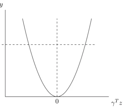
Example 3.1. Let p = 2. Assume that x = (x1, x2)T distributed uniformly on the unit circle kxk= 1. The true model is

y|x=x2₁+,

where the random error is independent of x. We observe that, since x2₁+x2₂ = 1,

y|x=x2₁+= (1−x2₂) +.

Thus, both S((1,0)T) and S((0,1)T) are dimension reduction subspaces. Because both of them are one dimensional subspaces, S((1,0)T) andS((0,1)T) are minimum DRSs.

The non-uniqueness of minimum dimension reduction subspaces could lead to erroneous

conclusions at later stages when we attempt to recover such minimum dimension reduction

subspaces. For instance, in the paper ofChiaromonte and Cook(2002), it is mentioned that

when using sliced inverse regression (Li, 1991) to recover minimum dimension reduction

subspaces for the example above, we often take the minimum dimension reduction subspace

as the intersection of S((1,0)T) and S((0,1)T), which is {0}. As a result, x and y are wrongly concluded to be independent.

To deal with the issues caused by non-uniqueness of minimum dimension reduction

sub-spaces, we adopt Cook’s idea (Cook, 1994a,b, 1996,2009). Cook introduced a new type

of space called central dimension reduction subspaces. When a regression has a central

dimension reduction subspace, the regression can only have a unique minimum DRS. Cook

suggested that we can avoid the problem of non-unique minimum DRSs by restricting our

attention to regressions for which the central dimension reduction subspace exists. We

give the formal definition of central dimension reduction subspaces below.

Definition 3.7(Central dimension reduction subspace). A subspaceSis a central dimen-sion reduction subspace (or central subspace for short) for the regresdimen-sion ofy on x ifS is a dimension reduction subspace and S⊆Sdrs for all dimension reduction subspaces Sdrs.

We denote the central dimension-reduction subspace by Sy|x orSy|x(Φ) when a matrix Φ

(43)

When a central subspace exists, it is the unique minimum DRS by definition. We can

formally prove this statement by contradiction. AssumeS1is a second minimum dimension

reduction subspace for an arbitrary regression with a central subspaceS_y|x. Then, because

Sy|x ⊆ S1 and dim(Sy|x) = dim(S1), we much have Sy|x = S1. Therefore, the central

subspace is the unique minimum DRS when it exists.

Nevertheless, it should be noted that a central subspace does not necessarily exist even

when there is a unique minimum dimension reduction subspace. To see this, we consider

a similar example but with p= 3.

Example 3.2. Let x∈_R3 _{be uniformly distributed on a unit sphere so that} _k_x_k_{= 1}_{. We} assume that

y|x=x2₁+.

For this example, the unique minimum direction reduction subspace S1 is spanned by the vector (1,0,0)T. However, since

y|x=x2₁+= 1−x2₂−x2₃+,

another possible dimension reduction subpsace S2 is spanned by vectors (0,1,0)T and

(0,0,1)T. The intersection of these two dimension reduction spaces is the origin.

In this case, the central subspace does not exist and the unique minimum dimension

reduction subspace is not a central subspace.

3.5 Existence of the central subspace

To follow Cook’s idea, it is important to identify conditions that ensure the existence of

the central subspace for regression problems. Apart from enabling us to decide whether

the results based on central subspaces are applicable to the regression problems of interest,

investigating these conditions also allow us to determine whether the class of regression

problems for which the central subspace exists is large enough for Cook’s idea to be of

practical use.

In order to study the existence conditions of the central spaces, we start by looking at a

(44)

Example 3.3. Letx∈_R3 _{be uniformly distributed on a unit sphere so that}_k_x_k_{= 1}_{. This} time, we modify the Example 3.2 slightly by letting

y|x=x2₁+x1+.

In this case, the central subspace exists and it is spanned by the vector (1,0,0)T. As the sign of x1 cannot be determined by x2 and x3, all possible dimension reduction subspaces must include the vector (1,0,0)T. Since the space spanned by (1,0,0)T is a dimension reduction subspace, it is by definition a central subspace.

This and Example3.2in the previous section show that the existence of a central subspace

depends on the conditional distribution of y|x and on the marginal distribution ofx. To further explore the conditions that affect the existence of a central subspace, we assume

that a problem of interest has a minimum dimension reduction subspace Sm(Φ) and we

also letSdrs(B) be an arbitrary dimension reduction subspace. Then, by the definition of

DRS, we have

y⊥⊥x|x, y⊥⊥x|ΦTx, y⊥⊥x|BTx.

Since BTx can be seen as a function of x and we know that y ⊥⊥x|ΦTx, Proposition 3.2

shows that

y⊥⊥x|(ΦTx, BTx).

Due to the equivalence between formulations (3.3) and (3.4), we thus have

Fy|x(a) =Fy|ΦT_x,BT_x(a) =F_y_|_ΦT_x(a) =F_y_|_BT_x(a), ∀a∈_R. (3.5)

The above equality is important because it helps us uncover essential relationships for

studying central subspaces. We observe that, given the equality(3.5), for alla∈R,

F_y|ΦT_x(a) =F_y_|_BT_x(a)

=E_ΦT_x_|_BT_x[F_y_|_ΦT_x,BT_x(a)] (by defn of conditional expectation)

=E_ΦT_x_|_BT_x[F_y_|_ΦT_x(a)].

(3.6)

Thus, the fact that Sm(Φ) and Sdrs(B) are dimension reduction subspaces implies that

F_y|ΦT_x(a) = E_ΦT_x_|_BT_x[F_y_|_ΦT_x(a)]. In other words, S_m(Φ) and S_drs(B) being dimension

(45)

F_y_|_ΦT_x(a) is constant with probability 1. So, no further information is supplied toF_y_|_ΦT_x(a)

by BTx given ΦTx.

The equality clearly holds when Sm(Φ) is a central subspace. That is Sm(Φ)⊂Sdrs(B).

However the equality (3.6) may hold under other conditions. If we can identify these

con-ditions, we may be able to force the existence of a central subspace by imposing restrictions

so that the equality (3.6) holds only when Sm(Φ) is a central subspace.

To explore different conditions for the equality (3.6), we start by assuming that Sm(Φ)

is not a central subspace. Without loss of generality, let S(C) := Sm(Φ)∩Sdrs(B) and

also letS(Φ1) =S(C)⊥S(Φ) andS(B1) =S(C)⊥S(B). Here, S(C)⊥S means the orthogonal

complement to S(C) in S. Since Sm(Φ) is not central, S(Φ1) and S(B1) are nontrivial

subspaces. Then, intuitively, the equality (3.6) implies that the information provided by

S(Φ1) to the response variable is the same as that provided byS(B1). To be more specific,

if the information about the response variable contained in S(Φ1) is contributed via a

function offΦ(ΦT1x), then there exists a functionfB(B1Tx) such thatfB(B1Tx) =fΦ(ΦT1x).

fΦ(ΦT1x) can be replaced by fB(BT1x).

Example 3.4. To better understand this statement, we recall Example 3.2. Let x ∈ _R3 be uniformly distributed on a unit sphere so that kxk= 1. We assume that

y|x=x2₁+.

In this case, Sm(Φ) = S((1,0,0)T), Sdrs(B) = S((0,1,0)T,(0,0,1)T) and S(C) = {0}. We also note that

fΦ(ΦT1x) =fΦ(ΦTx) = (ΦTx)2 =x21.

Moreover, since x follows a spherical distribution, we easily observe that by defining

fB(B1Tx) as

fB(B1Tx) =fB(BTx) := 1−x22−x23,

we can replace fΦ(ΦT1x) with fB(B1Tx). Here, we tie the regression function to the dis-tribution of x and thereby achieve the equality (3.6) without forcing the centrality. The possibility of replacement hence precludes the existence of a central subspace.

As a result, to ensure the existence of a central subspace, we have to eliminate the

(46)

fB(B1Tx), both functions fΦ and fB should be trivial. In order to enforce this

require-ment, we follow Chiaromonte and Cook (2002)’s approach and introduce a lemma from

real analysis first.

Lemma 3.8. Let Ω⊆_Rp _{be an open set, and} _g_:

Rp →R1 an analytic function. Also, let

PS be the orthogonal projection operator onS with respect to the standard inner product. Assume S1 and S2 are any two subspaces of Rp. Then if

g(x) =g(PS1x) =g(PS2x), ∀x∈Ω, (3.7)

we have

g(x) =g(PS1∩S2x), ∀x∈Ω. (3.8)

Proof. Let T =S1∩S2. In addition, let T1 =T⊥S1 and T2 =T⊥S2. T1 is the orthogonal

complement of T of the subspace S1 and T2 is the orthogonal complement of T of the

subspaceS2. Then for anyx∈Ω, we can decompose PS1x andPS2x as follows:

PS1x=PTx+PT1x,

PS2x=PTx+PT2x.

Here, we note thatPT1x and PT2xare linearly independent by the way they are defined.

Now, we recall the defining property for an analytic function g is that, for any a ∈ _Rp_,

one can write

g(z) =b0+ ∞ X

k1,...,kp=1

bk1,...,kp(z1−a1)k1. . .(zp−ap)kp (3.9)

where z is in the neighbourhood of a and b0, bk1,...,kp are constants. Leta =PTx. Then

by this property, we have

g(PS1x) =b0+ ∞ X

k1,...,kp=1

bk1,...,kp(u1)k1. . .(up)kp

and

g(PS2x) =b0+ ∞ X

k1,...,kp=1