Rochester Institute of Technology
RIT Scholar Works
Theses Thesis/Dissertation Collections
5-2015
Investigating the Effect of Color Gamut Mapping
Quantitatively and Visually
Anupam Dhopade
Follow this and additional works at:http://scholarworks.rit.edu/theses
This Thesis is brought to you for free and open access by the Thesis/Dissertation Collections at RIT Scholar Works. It has been accepted for inclusion
in Theses by an authorized administrator of RIT Scholar Works. For more information, please [email protected].
Recommended Citation
Investigating the Effect of Color Gamut Mapping Quantitatively and Visually
by Anupam Dhopade
A thesis submitted in partial fulfillment of the requirements for the degree of Master of Science in Print Media
in the School of Media Sciences in the College of Imaging Arts and Sciences
of the Rochester Institute of Technology
May 2015
Primary Thesis Advisor: Professor Robert Chung
School of Media Sciences Rochester Institute of Technology
Rochester, New York
Certificate of Approval
Investigating the Effect of Color Gamut Mapping Quantitatively and Visually
This is to certify that the Master’s Thesis of Anupam Dhopade
has been approved by the Thesis Committee as satisfactory for the thesis requirement for the Master of Science degree
at the convocation of May 2015 Thesis Committee:
__________________________________________
Primary Thesis Advisor, Professor Robert Chung
__________________________________________
Secondary Thesis Advisor, Professor Christine Heusner
__________________________________________
Graduate Director, Professor Christine Heusner
__________________________________________
iii
ACKNOWLEDGEMENT
I take this opportunity to express my sincere gratitude and thank all those who have supported me throughout the MS course here at RIT. Without you, I would have never been able to successfully complete the requirements of my MS degree.
To my thesis advisor, Prof. Robert Chung, I sincerely appreciate the endless support from you during my thesis and throughout my MS course at RIT. It was a pleasure to learn from you. You have always been available whenever I required your guidance. Thank you very much Prof. Chung!
To my thesis guide, Franz Sigg, who has been a constant source of guidance, encouragement, and inspiration throughout my MS course at RIT. I have learned so many things from you, not limited to studies, but also about life. I will cherish several
discussions I have had with you, your unconditional support, and your selfless attitude that you practiced since I have ever known you. Thank you so much Franz!
I would also like to thank Prof. Christine Heusner, who stepped in as my new secondary thesis advisor, guided me and helped coordinate the necessary actions with everyone in the committee so as to get my thesis completed. Thank you Prof. Heusner!
iv
you pappa! I would also like to thank my elder sister Pranita, and my brother in law Prakash for always encouraging me. I would also like to thank my dear wife, Preeti, for always standing by me, with her unconditional support through the good and bad.
v
Table of Contents
ACKNOWLEDGEMENT ... iiv
List of Tables ... vii
List of Figures ...viii
Abstract ... ix
Chapter 1: Introduction ... 1
Statement of the Problem ... 1
Significance of the Topic... 4
Reason for Interest in the Topic ... 4
Glossary of Terms ... 4
Chapter 2: Literature Review ... 9
Conceptual Stages of Gamut Mapping ... 9
GMA Building Blocks ... 10
Gamut Mapping Complexities ... 13
Chapter 3: Research Questions and Limitations of This Research ... 16
Research Questions ... 16
Limitations of this Research ... 17
Chapter 4: Methodology ... 18
Methodology for Research Question 1 ... 18
vi
Chapter 5: Results ... 28
Results for Research Question 1 ... 28
Results for Research Question 2 ... 37
Chapter 6: Summary and Conclusions ... 39
Future Research ... 40
BIBLIOGRAPHY ... 42
Appendix A: Monaco Profiler 5.0 Analysis...A1
vii List of Tables
Table 1: Most notable observations for differences in perceptual rendering intent for the two profiling applications ... 33 Table 2: Most notable observations for differences in colorimetric rendering intents for the
two profiling applications ... 35 Table 3: Most notable observations for differences in saturation rendering intent for the
viii List of Figures
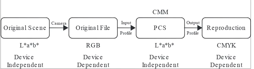
Figure 1: Workflow for color managed printing of an original scene seen by an eye...2
Figure 2: Sigg’s graphic test results for one of the hue slices for Saturation Intent...12
Figure 3: Sample Testform from real world colors for gamut mapping...20
Figure 4: Sample L*C* graph showing gamut mapping...21
Figure 5: Sample a*b* graph showing gamut mapping...22
Figure 6: Sample Gray axis plot...23
Figure 7: CIELab SCID images stacked into a block in Adobe Photoshop...24
Figure 8: CIELab SCID image blocks paired besides each other per rendering intent...25
Figure 9: Sample L*C* graphs for eight hue angles 45º for 'PM_Def_PaperGr_Classic_Np.ICC' from Gretagmacbeth Profile Maker 5.0...29
ix Abstract
With the advent of various color management standards and tools, the print media industry has seen many advancements aimed towards quantitatively and qualitatively acceptable color reproduction. This research attempts to test one of the most fundamental and integral parts of a standard color management workflow, the profile. The gamut mapping techniques implemented by the ICC profiles created using different profiling application programs were tested for their congruity to the theoretical concepts, standards, and definitions documented by International Color Consortium (ICC). Once these
profiling software applications were examined, the significance of the possible
discrepancies were tested by establishing a visual assessment of pictorial images using these profiles.
In short, this research assessed the implementations of the ICC color rendering intents in a standard or a commonly used color managed workflow, and then described the significance of these discrepancies in terms of interoperability. For this research, interoperability was defined the assessment of different ICC profiles in producing similar results, i.e., quantitatively and visually.
x
1 Chapter 1
Introduction
Statement of the Problem
The International Color Consortium (ICC) was established in 1993 with an aim to standardize the color management process and promote standardization of cross platform and vendor neutral files used in a color managed workflow. They developed a protocol for color definition between device values and the device-independent color called ‘profiles’ which allowed linking cross-platform devices in a single workflow and hence increase the efficiency of color management workflows.
2
Figure 1: Workflow for color managed printing of an original scene seen by an eye.
As clearly visible from the workflow, the scene is captured by a camera (a scanner is used in cases where the original is a photograph or a tangible flat surface) and converted to ‘device digital information’ and this device-dependent information is embedded with an input profile that helps the color management module or the ‘engine’ understand the nature of the color information. In other words, the engine is able to convert the device-dependent color information to device-independent color information in the profile connection space (PCS), which acts as a hub for color transformation.
The L*a*b* color space was introduced as the PCS, as it was larger than any color space that a device could have and was also considered to be visually uniform by the ICC. ICC laid out a simple framework for an open loop color management workflow, which was readily accepted by the print media industry and has been used for the last two decades.
Although ICC’s framework for open loop color management was simple, the process of gamut mapping is still complex. When mapping color from a larger gamut
pendent
Device
Independent IndDeepveincedent DeDpeevnidceent
ICC ColorManagement Workflow for printing from an originalscene
OriginalScene Camera OriginalFile Input PCS Reproduction
Profile
Output
Profile
L*a*b* RGB L*a*b* CMYK
CMM
Device
3
(e.g., RGB) to a smaller gamut (e.g., CMYK), clipping and compressing of the gamut is necessary. This can be done in different ways and is up to the color scientist to design the algorithms for the color mapping program that do these conversions in a way that
optimizes a specific color rendering intent between original and reproduction.
Recognizing this situation, ICC laid the framework and the general outline of the process, but did not define the specific algorithm thereby allowing individual programmer’s creativity in the form of trade secrets. ICC introduced four rendering intents which defined the end results for different image categories. But ICC entirely left it to the profiling application program designer’s choice to achieve the required results and what principle to be used. This also means there is not necessarily a correct or an incorrect way of doing gamut mapping.
There are many possible gamut mapping solutions. The user who may be a print operator, or a color expert does not really know what is under the hood and needs to rely on the vendors of the application programs required for creating the ICC profiles.
Moreover vendors do not reveal or document the entire logic of their programs. Several interesting questions arise such as:
• What are the different ways of handling the out of gamut colors?
• If the paper base has a color, how is it accounted for in different rendering intents?
• Is the gamut compressed linearly or non- linearly?
• During compression or clipping, is the lightness of the color preserved?
4
So there is no clear and easy method to identify how these differences may impact the quality of the printed products. Any user may want to know the answers to such questions before investing in a profiling application.
Significance of the Topic
A user spends approximate $3,000 to $5,000 for buying a profiling program of his choice, and similarly upgrading these programs costs more money. But he or she may not know if that particular program is better than the others for a given application. Due to all the above mentioned reasons and questions, it would be interesting to understand what really happens in the gamut mapping process.
Reason for Interest in the Topic
Being a student and having access to different profiling programs, it is possible to carry out the tests of interest and do a systematic comparison that the people in the print industry may not be able to do.
Glossary of Terms
5
Color Gamut
“Solid in a colour space, consisting of all those colours that are present in a specific scene, artwork, photograph, photomechanical or other reproduction; or are capable of being created using a particular output device and/or medium"(ISO 12640-3, 2005).
Color Gamut Mapping
“The process of converting colors from one color space to another is called as gamut mapping” (Sharma, 2003).
Gamut Mapping Algorithms (GMA)
“An algorithm for assigning colours from the reproduction medium to colours from the original medium or image (Morivic & Luo, 1997).
Color Management Module (CMM)
“The CMM, often called the engine, is the piece of software that performs all the calculations needed to convert the RGB or CMYK values” (Sharma, 2000).
Profile Connection Space (PCS)
6
Profile
“File containing data between device space and PCS in the form of matrix or look up tables (LUT). Profiles are classified as input and output based on the devices, or source and destination based on their roles in the workflow” (Chung, 2010).
Forward device characterization model
A forward transformation that takes device digital counts (e.g. a display's RGB or a printer's CMYK) and transforms it into a colorimetric description for specific viewing conditions (Morovic, 2008). Also known as A2B mapping when mapping to profile connection space.
Inverse device characterization model / Inverse Routine
An inverse transformation takes the colorimetric description for a specific viewing condition and transforms it back into destination device digital counts (Morovic, 2008). Also known as B2A mapping when mapping from profile connection space.
Rendering Intent
7
Perceptual Rendering Intent
“This rendering intent is useful for general reproduction of pictorial images, typically includes tone scale adjustments to map the dynamic range of one medium to that of another, and gamut warping to deal with gamut mismatches” (ICC specifications ver.2).
Saturation Rendering Intent
“This rendering intent is useful for images which contain objects such as charts or diagrams, usually involves compromises such as trading off preservation of hue in order to preserve the vividness of pure colours.” (ICC specifications ver.2).
Absolute Colorimetric Rendering Intent
"Absolute colorimetric differs from relative colorimetric and maps source white to destination white. Absolute colorimetric rendering from a source with a bluish white to a destination with yellowish-white paper puts cyan ink in the white areas to simulate the white of the original” (ICC specifications ver.2).
Media Relative Colorimetric Rendering Intent
8
Measurement and Perception of Color
A color is usually measured spectrally using a spectrophotometer. This device provides a reading every 5nm or 10nm, generally from 380nm to 730nm and this data can be
repurposed to calculate other data. The phenomenon of sensation of color depends on the object, illuminant and observer. The perception of color, on the other hand, heavily depends on various factors such as the spectral distribution of illuminant, the ambient lighting, the surrounding, surface characteristics, psychological and cultural influence etc. Hence a certain color object appears differently under different conditions. This
sometimes results in cases where considerable quantitative differences in measurements render just noticeable visual differences, while minute quantitative discrepancies
9 Chapter 2
Literature Review
The primary focus of this research was to visualize and illustrate to an average user what the profiling programs actually do in terms of gamut mapping. Therefore it does not involve color scientific discussions but simple language and easy to understand graphics. This literature review summarizes the previous relevant research related to gamut mapping. The issues included in this review were:
1) Conceptual stages of gamut mapping
2) Gamut Mapping Algorithm building blocks / Conditions for gamut mapping 3) Gamut mapping complexities
4) Real world gamut of surface colors. ISO 12640-3
Conceptual Stages of Gamut Mapping
Identifying several problems in the gamut mapping algorithm, the CIE has established a technical committee ‘CIE:TC8-03 Gamut Mapping’ under the supervision of Jan Morovic (2004). CIE TC08-03 has been established based on the work of Morovic where he surveyed more than 90 gamut mapping algorithms and provided a greater understanding of the intricacies involved in the gamut mapping process. Morovic and his committee members have been pursuing the aim of developing a universal gamut
10
and a critical part of any color management system by stating “Gamut mapping takes place in the context of a color reproduction process that can be implemented by means of a color management system..there are a variety of color management architectures that implement the conceptual stages of color reproduction in different ways, but that all of them need to provide gamut mapping functionality in at least one place” (p.90).
Morovic (2008) described color gamut mapping as having three conceptual stages where the first stage is the prediction of the visual appearance of the original
(characterization); the second stage, making changes to the original to compensate for the inevitable changes expected in destination color space (conversion to PCS); and final stage, predicting destination device’s color values (inversion routine).
Morovic’s experiment offers a wide range of areas worth researching. For this thesis, the scope of experiments will be limited to only the second stage mentioned above.
GMA Building Blocks
11
process by incorporating an optimized color transformation matrix, and reiterating the objective function a number of times.
Morovic explains that there are several aspects for consideration and
complexities involved in decision making while designing a gamut mapping algorithm. He shows how different designers may come up with different solutions while none are right or wrong. According to Morovic (2008: 105), there might be several gamut mapping algorithms available based on different principles and rules, including but not limited to single dimension mapping, mapping towards the point on lightness axis, or off lightness axis, mapping towards predetermined properties, interpolating or morphing, linear mapping, non-linear mapping, tetrahedral or distance weighted morphing, and numerous other considerations.
The argument presented by Nakauchi (1999) is: can the algorithm produce color accurately and pleasantly through all scenarios? The question implies that different algorithms are capable of producing excellent results in some applications while they might not produce the same quality of results for others. Therefore, the profiling program designers must modify or tweak to make it more adaptable by providing different settings. When a user selects one of the given settings in the program he/she might be
implementing different rules of mapping.
12
ranks them. However, Sharma does not focus on the reasons causing the differences. The author leads the reader to think more about the profiles which are the only variable in the workflows tested.
[image:23.612.199.451.335.550.2]On the other hand, Sigg (2005) details the differences in how the colors are mapped and leaves it to the reader to observe and conclude based on detailed graphs. For instance, the graph shown in Figure 2 presents a profile from a well-known profiling software implementing ‘saturation rendering intent’ does almost the opposite than what the theory says.
Figure 2: Sigg’s graphic test result for one of the hue slices for Saturation Intent
13
nonlinearly; and (3) the reproducible colors are not forced to the gamut boundaries, but darkened and desaturated. In theory, colors outside the gamut must be clipped and the ones inside the gamut must be forced towards the boundary of the gamut. This research identifies such issues and investigates the gamut mapping algorithms using graphs and simple language.
Identifying the need of such research and tests, ISO 12640-3 compiled a set of standard digital images and a list of real world colors that would be useful for:
1. Evaluating the color reproduction of imaging systems 2. Evaluating color image output devices
3. Evaluating the effect of image processing algorithms applied to the images 4. Evaluating the coding technologies necessary for the storage and transmission of
high-definition image data
This provides an idea of what the gamut of the original could be and how much compression or clipping would be required and an overview of the original color values. Using the color data list from this ISO 12640-3 standard would provide this research a strong base to start with, and using graphs such as shown in Figure 4, it would be easy to help the reader understand different complexities involved in the gamut mapping process.
Gamut Mapping Complexities
14
and considered as problems as they produce mathematical complexities in the gamut mapping computational process (Rosen, 2009). Some are:
Concavity of the gamut hull confuses the gamut mapping algorithms and often produces
wrong values or duplicate values for adjacent numbers. In such case, the matrices are algebraically inflated to compensate for; but this requires a lot of assumptions and is not desirable.
Overlapping of slices/hulls is also undesirable since the same input value is computed for
differently and produces two different values. (Usually a gamut is divided into sectors or slices at different hue angles, for making the computations simpler and then merged again).
Method of compression is one of the most challenging issues that needs to be handled.
Would a linear compression, be preferable or a bilinear compression, to preserve the saturation levels of most colors? When calculating the compression should L* be
15
16 Chapter 3
Research Questions and Limitations of This Research
Research Questions
Usually, a typical press operator using color management techniques seldom understands all the computations executed in a color managed workflow, including under the hood of a profiling application. In addition, since there is no correct or incorrect method of executing the gamut mapping, it becomes not only interesting but also necessary to exemplify different ways being used, explain the logic implemented, and determine if these procedures result in visually noticeable differences in the printed product. This research focused on the following questions:
Q1) How different are the selected profiling application programs in B-to-A
mapping for a given CMM under perceptual rendering intent? How different are the
profiling applications in B-to-A mapping under absolute, relative and saturation
rendering intents?
17
However, quantitative color difference displayed by the method above may not translate to visual color difference. This leads to the second research question:
Q2) Even if there are quantitative color differences due to different color mapping,
are the color differences visually noticeable in pictorial samples?
By answering the second research question with the use of SCID images in CIELAB color space, it will be clear to the reader that existence of several different methods of gamut mapping techniques might lead to different visual appearances.
Limitations of this Research
• A single CMM, CHROMiX ColorThink’s CMM, is used in the experiment
• The round-trip (B-to-A-to-B) is used to implement the gamut mapping with the assumption that the A-to-B conversion, which takes place after the gamut mapping, is colorimetrically accurate.
18 Chapter 4
Methodology
Methodology for Research Question 1
Q1) How different are the selected profiling applications in B-to-A mapping for a
given CMM under perceptual rendering intent? How different are the profiling
applications in B-to-A mapping under absolute, relative and saturation rendering intents? To obtain a clear explanation for the first research question, the following
19
The procedure for testing is as follows:
1) It must be understood that a large amount of gamut compression and clipping is preferable. Since this study is about understanding gamut clipping and
compression, the destination gamut selected should be of a smaller size so as to make the effect of gamut compression and clipping more evident. In doing so, this will amplify the effects of gamut mapping, and make it easy for the observer to draw inferences and conclusions. To achieve maximum compression and clipping, the profiling testform could be printed on an uncoated grayish paper with a low whiteness and brightness value, such as newsprint paper. But this introduces several variables such as mottle and poor repeatability of the process. Instead, a standard characterization data set for newsprint paper were used to create the profiles using the profiling software. ‘ISOnewspaper26v4.icc’ data set will be acquired from ‘World Association of Newspapers and News Publishers’ website – ‘www.wan-ifra.com’, for this purpose. This eliminates all the variables related to printing the profiling test target and therefore provides more reliability to the procedure.
20
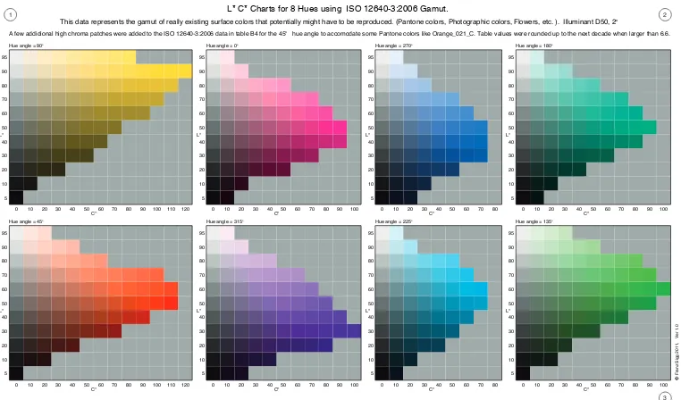
Figure 3: Sample Testform from real world colors for gamut mapping.
3) The testform shown in the Figure 3 with eight hue slices 45° apart, created by Franz Sigg, will be used for testing the profiles. The testform contains only ‘real world colors’ as stated by ISO 12640-3. The colors in this testform were defined in the CIELab space (PCS) and hence it is device independent color information. 4) The data from this testform was then converted by the profiles which were created
using different profiling programs using CHROMiX ColorThink Pro 3.0 with its CMM. The conversion returns in device L*a*b* color values.
5) The obtained device L*a*b* values were then compared with input L*a*b* values from the testform. By the end of step 4, a round-trip conversion was obtained, where the inversion (B-to-A) and the forward (A-to-B) routines were performed with gamut mapping as an integral part of these steps.
L* C* Charts for 8 Hues using ISO 12640-3:2006 Gamut.
This data represents the gamut of really existing surface colors that potentially might have to be reproduced. (Pantone colors, Photographic colors, Flowers, etc. ). Illuminant D50, 2o
Franz Sigg 2011, Ver 1.0
A few addidional high chroma patches were added to the ISO 12640-3:2006 data in table B4 for the 45o hue angle to accomodate some Pantone colors like Orange_021_C. Table values were rounded up to the next decade when larger than 6.6.
1 2 3 L* 5 10 20 30 40 50 60 70 80 90 95
0 10 20 30 40 50 60 70 80 90 100110120 C*
Hue angle = 90o
L* 5 10 20 30 40 50 60 70 80 90 95
0 10 20 30 40 50 60 70 80 90100 C*
Hue angle = 0o
L* 5 10 20 30 40 50 60 70 80 90 95
0 10 20 30 40 50 60 70 80 C*
Hue angle = 270o
L* 5 10 20 30 40 50 60 70 80 90 95
0 10 20 30 40 50 60 70 80 90 100 C*
Hue angle = 180o
L* 5 10 20 30 40 50 60 70 80 90 95
0 10 20 30 40 50 60 70 80 90 100110120 C*
Hue angle = 45o
L* 5 10 20 30 40 50 60 70 80 90 95
0 10 20 30 40 50 60 70 80 90100 C*
Hue angle = 315o
L* 5 10 20 30 40 50 60 70 80 90 95
0 10 20 30 40 50 60 70 80 C*
Hue angle = 225o
L* 5 10 20 30 40 50 60 70 80 90 95
0 10 20 30 40 50 60 70 80 90 100 C*
21
[image:32.612.225.422.313.473.2]6) From the two profiles, the converted data sets for all the four rendering intents were plotted on an L*C* graph, a*b* graph, tone reproduction graph, and gray axis graph as shown in Figure 4, Figure 5, and Figure 6 respectively. These graphs show how the gamut mapping is applied to the eight different hue slices. From the sample graphs shown in Figure 6, and Figure 7, it can be easily seen how the real world colors converge from a larger gamut to a smaller gamut. The L*C* graphs will be generated for eight different hue angles, as mentioned previously, revealing the specifics of the gamut mapping algorithm.
22
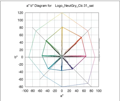
Figure 5: Sample a*b* graph showing gamut mapping.
The a*b* graph in Figure 5, shows the original gamut and the destination gamut and also shows the colors at the eight hue angles, giving a clear idea about the gamut of the saturated colors. This graph also shows that the fully saturated colors, moving from the white point to the black point for each hue angle do not
necessarily maintain a constant hue angle. Each color is shown using closest hue and darkness in the graph, therefore darker lines represent colors with low L* values, while lighter lines represent colors with higher L* values.
a* b* Diagram for Logo_NeutGry_Clc 31_sat
-80 -60 -40 -20 0 20 40 60 80 100 120
b*
Fr
anz Sigg 2
004, Ver 3
.7, Lice
nsed
user: Not Valida
ted
a*
23
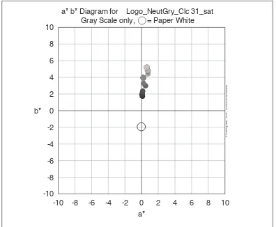
Figure 6: Sample Gray axis plot
In addition to this, the gray axis will also be plotted as shown in Figure 6 which displays the axis shift or the whitepoint shift.
7. To list significant quantitative color differences from the observations off the graphs and the available quantitative data.
Methodology for Research Question 2
Q2) Even if there are quantitative color differences due to different color mapping,
are the color differences noticeable when examining the samples visually? The objective of answering question 2 is to verify if a systematic analysis of
subjective responses would substantiate a conclusive finding. Employing simulation at all stages was one of the objectives to not only reduce the cost of this research but also to consistently retain use of printing standards throughout the research and offer more
a* b* Diagram for Logo_NeutGry_Clc 31_sat Gray Scale only, = Paper White
-10 -8 -6 -4 -2 0 2 4 6 8 10
b*
Franz Sigg 2004, Ver 3.7, Licensed user: Not Validated
a*
24
flexibility. As a part of the preparation for the experiment, the following steps were followed:
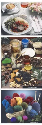
[image:35.612.283.365.254.495.2]1) Three pictorial images from the group of ISO CIELab SCID images were selected which covered most hues and also had intricate details that would be affected due to gamut size. The selected images were 'N3_16_LAB_r', 'N4_16_LAB_r', and 'N7_16_LAB_r', as shown in Figure 7.
Figure 7: CIELab SCID images stacked into a block in Adobe Photoshop 2) The selected CIELab SCID pictorial images were opened in Photoshop and a
block of all three images was created as shown in Figure 7 above.
25
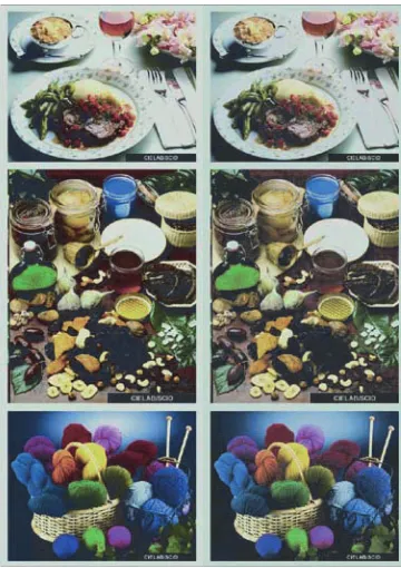
[image:36.612.233.413.198.453.2]4) Each image was converted to Adobe RGB, with absolute rendering intent, in order to produce a common comparing color space but also preserve the gamut compressions and clippings caused by the respective profiles and rendering intents.
Figure 8: CIELab SCID image blocks paired besides each other per rendering intent 5) In MS PowerPoint 2007, a comparison set of two blocks from both the profiling
applications for each rendering intent was assembled, resulting in four
comparison sets. Each comparison set (as shown in Figure 8) consisted of two blocks of the three CIELab images converted to profiles from Monaco Profiler and Gretagmacbeth ProfileMaker.
6) Such assemblies when displayed on an ISO 12646 compliant monitor, such as an Eizo display, makes it very easy to compare and evaluate the tonality,
26
7) In the experiment, the observers were instructed to evaluate visual color
differences between the color image pairs. The questions were limited to be very basic and simple to understand so as not to confuse the observer.
8) The observers were shown the paired blocks for all four rendering intents one pair at a time. Each pair was shown to the observer as shown in Figure 8, twice and randomly sequenced without the knowledge of having been repeated or having known that there were only four distinct pairs.
9) All observers were instructed to “Pick one, block of images from the pair, that is
visually more chromatic/saturated colors than the other.”
10)The questions were conceived in such a way that the answers would help either to corroborate or refute the conclusion from question 1. Any ambiguity in the
answers could mislead the research into meaningless information and conclusions. 11)The observer would be considered consistent only when he/she picked the same
image block as one with visually more pleasing colors twice. This enabled the data from inconsistent observers to be identified and filtered out.
27
28 Chapter 5
Results
Results for Research Question 1
Q1) How different are the selected profiling application programs in B-to-A
mapping for a given CMM under perceptual rendering intent? How different are the
profiling applications in B-to-A mapping under absolute, relative and saturation
rendering intents?
In order to answer Q1, the following quantitative differences can be observed
based on the graphs produced by ‘Sigg’s Profile Analysis Tool version 45.’ The differences may not necessarily refer to significantly noticeable color differences, but may refer to observations that show unique rules /methods implemented by the profiling applications that influence the profile’s color conversions differently in each application. Before delving into the data, the most notable observations based on the ‘summary of profile analysis’ from ‘Sigg’s Profile Analysis Tool version 45’ are mentioned.
CHROMiX ColorThink Pro 3’s worksheet feature was used for converting the real world colors from ISO 12640-3 to the respective profiles. The following differences in Figure 9 are listed for CHROMiX ColorThink’s CMM which was used while
29
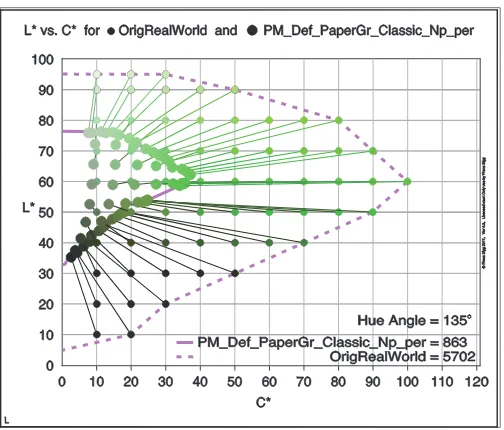
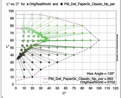
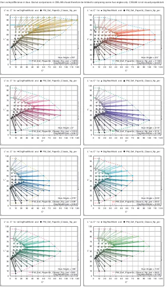
Figure 9: Sample L*C* graphs for eight hue angles 45º for
29
Figure 9: Sample L*C* graphs for eight hue angles 45º for
'PM_Def_PaperGr_Classic_Np.ICC' from Gretagmacbeth Profile Maker 5.0
CIELAB Data from LC_11U-6.6.EPS chart with ISO-WD 12640-3.4 colors was taken, and the PM_Def_PaperGr_Classic_Np.ICC profile was applied using ColorThink, first converting Lab to CMYK using Perceptual color rendering intent. Then, to simulate printing, this CMYK data file was converted back to Lab, using the same profile back to Lab using the same profile with Absolute rendering. The L*C* charts below show this data compared against the original Lab data from LC_11U-6.6.EPS. Note: The indicated gamut size numbers are in terms of L*C* CIELAB area units. It is well known that a step difference in yellow is visually less significant than a step difference in blue. Gamut comparisons in CIELAB should therefore be limited to comparing same hue angles only. CIELAB is not visually equidistant.
Perceptual Rendering, PM_Def_PaperGr_Classic_Np.ICC,
L 0 10 20 30 40 50 60 70 80 90 100
Franz Sigg 2011, Ver 4.3, Licensed user: Only use by Franz Sigg
0 10 20 30 40 50 60 70 80 90 100 110 C*
L* vs. C* for OrigRealWorld and PM_Def_PaperGr_Classic_Np_per
L*
120 Hue Angle = 90o
OrigRealWorld = 6280 PM_Def_PaperGr_Classic_Np_per = 1229
L 0 10 20 30 40 50 60 70 80 90 100
Franz Sigg 2011, Ver 4.3, Licensed user: Only use by Franz Sigg
0 10 20 30 40 50 60 70 80 90 100 110 C*
L* vs. C* for OrigRealWorld and PM_Def_PaperGr_Classic_Np_per
L*
120 Hue Angle = 45o
OrigRealWorld = 6301 PM_Def_PaperGr_Classic_Np_per = 1133
L 0 10 20 30 40 50 60 70 80 90 100
Franz Sigg 2011, Ver 4.3, Licensed user: Only use by Franz Sigg
0 10 20 30 40 50 60 70 80 90 100 110 C*
L* vs. C* for OrigRealWorld and PM_Def_PaperGr_Classic_Np_per
L*
120 Hue Angle = 0o
OrigRealWorld = 5351 PM_Def_PaperGr_Classic_Np_per = 1010
L 0 10 20 30 40 50 60 70 80 90 100
Franz Sigg 2011, Ver 4.3, Licensed user: Only use by Franz Sigg
0 10 20 30 40 50 60 70 80 90 100 110 C*
L* vs. C* for OrigRealWorld and PM_Def_PaperGr_Classic_Np_per
L*
120 Hue Angle = 315o
OrigRealWorld = 5726 PM_Def_PaperGr_Classic_Np_per = 574
L 0 10 20 30 40 50 60 70 80 90 100
Franz Sigg 2011, Ver 4.3, Licensed user: Only use by Franz Sigg
0 10 20 30 40 50 60 70 80 90 100 110 C*
L* vs. C* for OrigRealWorld and PM_Def_PaperGr_Classic_Np_per
L*
120 Hue Angle = 270o
OrigRealWorld = 4252 PM_Def_PaperGr_Classic_Np_per = 539
L 0 10 20 30 40 50 60 70 80 90 100
Franz Sigg 2011, Ver 4.3, Licensed user: Only use by Franz Sigg
0 10 20 30 40 50 60 70 80 90 100 110 C*
L* vs. C* for OrigRealWorld and PM_Def_PaperGr_Classic_Np_per
L*
120 Hue Angle = 225o
OrigRealWorld = 4351 PM_Def_PaperGr_Classic_Np_per = 663
L 0 10 20 30 40 50 60 70 80 90 100
Franz Sigg 2011, Ver 4.3, Licensed user: Only use by Franz Sigg
0 10 20 30 40 50 60 70 80 90 100 110 C*
L* vs. C* for OrigRealWorld and PM_Def_PaperGr_Classic_Np_per
L*
120 Hue Angle = 180o
OrigRealWorld = 5126 PM_Def_PaperGr_Classic_Np_per = 691
L 0 10 20 30 40 50 60 70 80 90 100
Franz Sigg 2011, Ver 4.3, Licensed user: Only use by Franz Sigg
0 10 20 30 40 50 60 70 80 90 100 110 C*
L* vs. C* for OrigRealWorld and PM_Def_PaperGr_Classic_Np_per
L*
120 Hue Angle = 135o
30
Figure 9 provides a sense of how some of the graphs appeared. Several other
graphs were used to deduce observations. The entire quantitative analysis summary of
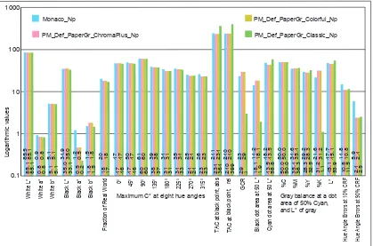
profiles is shown graphically in Figure 10 below. The full set, of these graphs, is shown
in the appendix.
Figure 10: Graphic summary of all three profiles from Gretagmacbeth Profile Maker 5.0,
and one profile from Monaco Profiler 5.0
It is known that CIELAB is not visually uniform (Hill et al.; 1997), hence step
differences for a certain hue can be visually less significant than step differences for
another hue, for ex. yellow and blue. Therefore, gamut comparisons in CIELAB in this
research are always limited to comparing same hue angles only. 0.1
1 10 100 1000
White L* White a* White b* Black L* Black a* Black b*
Fraction of Real World
Û Û Û Û Û Û Û Û
TAC at black point, abs TAC at black point, rel
GCR
Black dot area at 50 L* Cyan dot area at 50 L*
Hue Angle Errors at 10% CRF Hue Angle Errors at 90% CRF
Monaco_Np
PM_Def_PaperGr_ChromaPlus_Np
PM_Def_PaperGr_Colorful_Np
PM_Def_PaperGr_Classic_Np
%C %M %Y %K L*
Logarithmic values
Maximum C* at eight hue angles Gray balance at a dot area of 50% Cyan, and L* of gray
85.5 0.9 5.1 34.9 1.2 1.5 20 47 50 61 39 34 35 25 26 241 240 23 14.2 48.2 50.0 34.6 29.2 21.6 47.7 14.8 5.9
85.1 0.8 5.1 35.0 0.5 1.8 18 47 47 60 38 31 34 24 23 234 240 29 18.1 43.5 50.0 35.4 28.3 31.2 45.1 10.8 2.4
85.1 0.8 5.1 35.0 0.5 1.8 18 47 47 60 38 31 34 24 23 234 240 29 18.1 43.5 50.0 35.4 28.3 31.2 45.1 10.8 2.4
85.1 0.8 5.1 33.1 0.2 1.5 17 46 46 60 37 31 33 24 23 364 399 3 1.9 58.8 50.0 36.3 32.5 1.1 53.9 11.5 2.5
Fig . XX Summar y of Profiles per
[image:41.612.116.535.216.493.2]31
The most notable observations inferred from the two applications (Monaco Profiler 5.0 and Gretagmacbeth ProfileMaker 5.0) obtained from the graphical summary of profiles as shown in Figure 10 are:
a. White points for all the profiles were virtually the same.
b. Monaco Profiler had a slightly more red, but very negligibly different, black point as compared to that of ProfileMaker.
c. Even though the same data set was used to create the two profiles which result in the same gamut size for both profiles as per CHROMiX
ColorThink Pro, Sigg’s Profile Analysis Tool showed that Monaco Profiler had slightly greater reproducible percentage of real world colors. It was determined that the gamut size differences arise because the data set used to make the profiles (IT8-7.3) and the data set used for Sigg's Profile Analysis Tool are different, and therefore the gamut mapping algorithms have to interpolate, which they do differently.
d. For the same reason, Monaco Profiler showed an equal or slightly greater saturation (C*) of maximum saturated colors for all hue angles as
compared to ProfileMaker profiles.
32
defaults from the application. GCR in ProfileMaker’s Classic workflow is comparatively lower. It also uses a higher TAC.
f. Similarly, K component in GCR and K dot area at 50L* are significantly lower in the ProfileMaker Classic workflow.
g. With these observations, it is clear that the two profiling applications are different in various areas, although the three profiling workflows from ProfileMaker were similar to each other in most areas, except for GCR. Some of the L*C* graphs show some abrupt changes at the gamut
boundary which are assumed to be rounding problems due to the fact that the sampling steps for the L* and C* axes are relatively high at 10 units. They are not investigated any deeper, hence it is not conclusive whether there are complexities such as concavity, overlapping of colors (arising due to overlapping of gamut slices/hulls), and other erratic unexplainable behaviors.
h. On the basis of these observations, it was decided to pick the ProfileMaker ‘Classic’ workflow for comparisons with Monaco Profiler to answer both the parts of question Q1. Moreover, the remaining two profiling
workflows from ProfileMaker were quite similar, and hence would not add much to the understanding of the differences between the profiles. i. Considering the small magnitude of the differences in the two profiles, it
is possible to say that the two profiles can interoperate to produce the
33
The following differences are listed for CHROMiX ColorThink’s CMM, which was used while obtaining the round-trip L*a*b* data for the real world color test target using the profiles in the research.
The most notable observations inferred for the two applications (Monaco Profiler vs. ProfileMaker) for B-to-A mapping with respect to how the color conversions differ for perceptual rendering intent, were:
Table 1: Most notable observations for differences in perceptual rendering intent for the two profiling applications
Factors in comparison
Monaco Profiler ProfileMaker Classic
a. Chroma All eight hues have more chromaticity. Greens, yellows, oranges, and violets are significantly more saturated.
Lighter hues in highlights in blues, oranges, violets, cyan and green have more chromaticity. Hence, lighter colors will appear cleaner and more vivid.
b. Gamut
Compression and clipping with respect to L*
Lesser gamut
compression. All colors at 60<L*<70 retain same L* post clipping.
More gamut compression is notable. Gamut
[image:44.612.144.542.318.701.2]clipping for all hues above the cusp is smooth. Severe concavity (gamut complexity) is apparent in all the hues for colors below the cusp. (See Figure 9 or appendix.) c. Similarities within
application to other rendering intents.
Perceptual rendering intent is unique but relative colorimetric is same as saturation, which defies the definitions of the rendering intents as per the ICC specifications.
Perceptual is same as saturation, which defies the definitions of the rendering intents as per the ICC specifications.
d. Hue angle
34
most deviating and scattered. CRF curve of hue angle accuracy shows +/- 20 degrees deviation at 80% of real world colors. See Figure 10.
to be better retained. No considerable scattering is visible in any hues. High hue angle faithfulness is apparent. Up to 80% of real world colors only deviate by +/- 10 degrees, in the CRF curve.
e. Gray Reproduction Grays appear to be
approximately equidistant in a line.
Grays appear to show slight hooking at extreme low L* values, which may not contribute to any notable differences. f. Other observations Several colors are group-forced to same notable points
with same L* values on the gamut boundary (resulting in no color difference). This occurs even when the uncompressed colors have greater L* differences as compared to other colors that are mapped to discrete points on the gamut boundary.
In summation, the Monaco Profiler appears to sacrifice hue angle accuracy but preserves chromaticity, whereas ProfileMaker sacrifices chromaticity and retains maximum hue angle accuracy. Monaco Profiler produces a larger reproducible gamut than ProfileMaker, but it is difficult to state if hue angle accuracy is inversely
proportional to chromaticity. Therefore, it may be inferred that Monaco Profiler prioritizes more saturated colors over accurate colors whereas ProfileMaker prioritizes accuracy of colors over other gamut mapping parameters.
Next, the profiles for Monaco Profiler vs. ProfileMaker Classic will be discussed. The most notable observations from the two applications for B-to-A mapping are
35
Table 2: Most notable observations for differences in colorimetric rendering intents for the two profiling applications
Comparison for Absolute and
Relative Colorimetric
Monaco Profiler ProfileMaker Classic
a. Chroma All eight hues have
greater chromaticity. Hues have slightly lesser chromaticity. b. Hue Angle
accuracy Hues at each angle deviate in a random wavy pattern, which is of concern. Such an instant would be approvable only in cases where the profiling measurements used were randomly deviating (which they are not). Hue angle errors: at 10% CRF = -14.8 90% CRF = 5.9
Hues at each angle consistently show
minimum deviation from the ideal angle. Hue angle errors: at 10% CRF = -11.5
90% CRF = 2.5
c. Gamut
complexities in boundaries
More abrupt stepping is visible in the colors above the cusp, in all gamut slices
Concavities (an undesired gamut surface complexity) is consistently visible above the cusp, in all gamut slices
d. Profile settings (Black Point, TAC, GCR)
Slightly redder black point. TAC’s limited to 241%. GCR% used is 23%.
Darkest black point (33.1 L*). TAC’s sum up all the way to 399% for relative, and maximum GCR% used is only 3%.
Interestingly, the default ProfileMaker Classic black settings are similar to older conventional offset printing practices, which may be the reason why it is named “Classic” workflow. Monaco has greater gamut in darker areas.
36
[image:47.612.146.542.293.423.2]Table 3 presents the comparative analysis for saturation rendering intent. Interestingly, both profiling applications for saturation rendering intent appear to deviate from the definition as per ICC Specification Version 2 and have gamut mapping algorithms implemented based on customized definitions.
Table 3: Most notable observations for differences in saturation rendering intent for the two profiling applications
Comparison for Saturation Intent
Monaco Profiler ProfileMaker Classic
Unique
observations and conclusion
Saturation intent is the same as relative colorimetric rendering intent. Hence, it does not increase the saturation of within-gamut colors.
Saturation intent is the same as perceptual rendering intent. Hence, it does not increase the saturation of within-gamut colors, but preserves the
inter-relationship of all the colors.
37 Results for Research Question 2
Q2) Even if there are quantitative color differences due to different color
mapping, are the color differences noticeable when examining the samples visually?
Based on quantitative findings, the graphical data for the profile from Monaco Profiler displayed slightly more saturation than ProfileMaker. Whether a set of subjective responses produced a similar evaluation was of paramount interest. The results are
[image:48.612.104.531.376.650.2]presented in Table 4. The observations deliberately were not categorized per rendering intent, to avoid complex classifications and inability to draw meaningful conclusions.
Table 4: Total 80 observations from 20 observers twice for 4 rendering intents
C
onsi
ste
nt O
bse
rv
ati
on
s
Mon
ac
o
P
rof
il
er
5.
0
Observers to consistently pick Monaco Profiler 5.0 image
block, out of 4 image blocks, as one with 'visually more
chromatic/saturated colors'
12
G
ret
agm
ac
b
et
h
P
rof
il
eMak
er
5.
0 Observers to consistently pick Gretagmacbeth
ProfileMaker 5.0 image block, out of 4 image blocks, as
one with 'visually more chromatic/saturated colors'
09
Inc
ons
is
te
nt
O
bs
er
vati
ons
Inconsistent observers to pick both ProfileMaker and
Gretagmacbeth ProfileMaker 5.0 image blocks as ones
with 'visually more pleasing colors' for the same images,
when the same images were shown twice
38
With these findings, the outcome of the visual comparisons failed to substantiate any differences between the two. Almost 75% of observers were unable to choose one block of images over the other and hence were categorized as 'inconsistent'. From the remaining approximate 25% of the observations, it was not conclusive if the observers favored either Monaco Profiler or ProfileMaker. Since most color-aware observers could not discern the color difference consistently in the psychometric experiment, we conclude that there is no real visual differences among the samples represented by different gamut mapping and profiling software packages. With such findings, it was deemed
39 Chapter 6
Summary and Conclusions
The quantitative data revealed that Monaco Profiler produces slightly more saturated colors than Profile Maker. However, the question of interest is whether this could be confirmed by an analysis of subjective visual responses. The answer was no. The subjective responses revealed that the observations were not conclusive enough to corroborate the finding that the images color managed by Monaco Profiler were more chromatic or more saturated. The observers were not able to consistently pick the same images, which may be due to the fact, that visually, there were no significant color differences between the samples.
40
The answer to question Q1 indicates that there are small measurable differences in gamut sizes, inter-relationship between L* and hue angles for input colors and
compressed colors, default total ink limits, and default GCR settings. However, the answer to question Q2 suggests that those differences were visually insignificant. The two profiles are interoperable when evaluated visually.
Readers should benefit from this research as it displays how a seemingly
impenetrable topic can be investigated without delving too much into the cores of physics and mathematics. The graphical representation of the data is quite detailed and
informative, and may help readers to use these graphing techniques in their research. Lastly, readers will benefit by having the insight of where this research was able to evaluate differences between profiles, and where there were shortcomings.
Future Research
41
42
BIBLIOGRAPHY
Braun, G.J. & Fairchild, M.D. (2000). General-purpose gamut-mapping algorithms: Evaluation of contrast-preserving rescaling functions for color gamut mapping. Journal of Imaging Science and Technology, 44, 4, 343-350.
Chung, R. & Yoshikazu, S. (2001). Quantitative analysis of pictorial color image difference. In 2001 TAGA Proceedings, (pp. 381-398).
Dugay, F, Farup, I, Hardeberg, J. Y. (2008). Perceptual evaluation of color gamut mapping algorithms. Color Resolution & Application, 33, 470-476.
Fairchild, M. (1998). Color Appearance Models. , Reading, MA: Addison–Wesley.
Hunt, R.W.G. (2004). The Reproduction of Colour, 6th Ed. Chichester, England: Wiley, 2004.
ICC (2003-09). International Color Consortium. Specification ICC.1:2004-10 (Profile version 4.2.0.0). Image technology colour management — Architecture, profile format, and data structure [REVISION of ICC.1:2003-09].
ISO 12640-3 Graphic technology — Prepress digital data exchange — Part 3: CIELAB standard colour image data (CIELAB/SCID). First edition, Reference number ISO/IEC
43
Kang, B.H., Cho, M.K.,Choh, H.K. & Kim, C.Y. (2005). Perceptual gamut mapping on the basis of image quality and preference factors. In (editor?) Society of
Photographic Instrumentation Engineers Proceedings, 2058, 2005.
Kang, B.H., Morovic, J., Ronnier Luo, M., & Cho, M.S. (2003). Gamut compression and extension algorithms based on observer experimental data, Electronics &
Telecommunication Research Institute, 25, 158-168.
Kolas, O., & Farup, I. (2007). Efficient hue-preserving and edge-preserving spatial color gamut mapping. In 15th color imaging conference; color science and engineering systems, technologies and applications (pp 207-212). Springfield, VA, USA: Society for Imaging Science and Technology.
Kotera, H., Suzuki, M., Mita, T., & Saito, R. (2002). Image-dependent color mapping for pleasant image renditions. Society of Photographic Instrumentation Engineers Proceedings, 4421: p.461-464, 2002.
Lee, C.S., Lee, C.H., and Ha, Y.H. (2000). Parametric gamut mapping algorithms using variable anchor points. Journal of Imaging Science & Technology, 44,1, 68- 89.
MacDonald, L., Morovic, J. & Xiao, K. (2001). Evaluation of a Colour Gamut Mapping Algorithm, Association Internationale de la Couleur Proceedings, 4421: p.452-459, 2001.
Montag, E.D., and Fairchild, M.D. (1998). Gamut mapping: Evaluation of chroma clipping techniques for three destination gamuts. Imaging Science & Technology: Color & Imaging Conference 6, p.57-61.
44
Morovic, J. (2008). Color gamut mapping. Chichester, England: John Wiley & Sons.
Morovic, J., and Luo, M.R. (1998). Verification of gamut mapping algorithms in CIECAM97s using various printed media. Imaging Science & Technology: Color &
Imaging Conference 6, 53-56.
Nakauchi, S., Hatanaka, S., Usui, S. (1999). Color gamut mapping based on a perceptual image difference measure. Color Resolution & Application., 24, 280-291.
Ploumidis, D. (2005). Device link profiling. Test Targets 5.0, (pp.1 8-25). Accessed from http://scholarworks.rit.edu/books/73
Rosen, M., (2009). Color Gamut Mapping, Course Notes of RIT’2009: Color Systems, College of Imaging Science, Rochester Institute of Technology, USA.
Ridder, H., & Blommaert, F.J.J. (1995). Naturalness and image quality: chroma and hue variation in color images of natural scenes. Society of Photographic
Instrumentation Engineers Proceedings,, 2411, p.51-61.
Sharma G. (2003). Digital color handbook. Boca Raton, FL : CRC Press.
Sharma, A., & Fleming P. (2002, April). Evaluating the quality of commercial ICC color management software, WMU ICC Profiling Review 1.1.Presented at TAGA Technical Conference, North Carolina.
Sharma A., & Fleming, P. (2002). Measuring the quality of ICC profiles and color
45
Western Michigan University, WMU ICC Profiling Review 1.2. Retrieved from http://www.aldertech.com/pdfs/WMU_Profiling_Review_2.0.pdf
Sharma, A., & Fleming, P. (2002). Evaluating the quality of commercial ICC color management software, WMU ICC Profiling Review 1.3. Seybold Report, 2, (19) 3-9..
Sigg, F. (2005). Comparing performance of output profile making programs: A look at performance of different color mapping algorithms for rendering intents. Retrieved from Sigg, F.
Stone, M.C., Cowan, W.B., & Beatty, J.C. (1998). Color gamut mapping and the
printing of digital color images. ACM Transactions on Applied Perception proceedings, 7, 4, 249-292, 1988.
Wolski, M., Allebach, J.P., & Bouman, C.A. (1994). Gamut mapping: Squeezing the most out of your color system. Imaging Science & Technology: Color & Imaging Conference 2, p.89-91.
46
CIELAB Data from LC_11U-6.6.EPS chart with ISO-WD 12640-3.4 colors was taken, and the Monaco_Np.ICC profile was applied using ColorThink, first converting Lab to CMYK using Relative color rendering intent. Then, to simulate printing, this CMYK data file was converted back to Lab, using the same profile back to Lab using the same profile with Absolute rendering. The L*C* charts below show this data compared against the original Lab data from LC_11U-6.6.EPS.
Note: The indicated gamut size numbers are in terms of L*C* CIELAB area units. It is well known that a step difference in yellow is visually less significant than a step difference in blue. Gamut comparisons in CIELAB should therefore be limited to comparing same hue angles only. CIELAB is not visually equidistant.
Relative Rendering, Monaco_Np.ICC,
XR 0 10 20 30 40 50 60 70 80 90 100
Franz Sigg 2011, Ver 4.3, Licensed user: Only use by Franz Sigg
0 10 20 30 40 50 60 70 80 90 100 110 C*
L* vs. C* for OrigRealWorld and Monaco_Np_rel
L*
120 Hue Angle = 90o
OrigRealWorld = 6280 Monaco_Np_rel = 1467
XR 0 10 20 30 40 50 60 70 80 90 100
Franz Sigg 2011, Ver 4.3, Licensed user: Only use by Franz Sigg
0 10 20 30 40 50 60 70 80 90 100 110 C*
L* vs. C* for OrigRealWorld and Monaco_Np_rel
L*
120 Hue Angle = 45o
OrigRealWorld = 6301 Monaco_Np_rel = 1448
XR 0 10 20 30 40 50 60 70 80 90 100
Franz Sigg 2011, Ver 4.3, Licensed user: Only use by Franz Sigg
0 10 20 30 40 50 60 70 80 90 100 110 C*
L* vs. C* for OrigRealWorld and Monaco_Np_rel
L*
120 Hue Angle = 0o
OrigRealWorld = 5351 Monaco_Np_rel = 1226
XR 0 10 20 30 40 50 60 70 80 90 100
Franz Sigg 2011, Ver 4.3, Licensed user: Only use by Franz Sigg
0 10 20 30 40 50 60 70 80 90 100 110 C*
L* vs. C* for OrigRealWorld and Monaco_Np_rel
L*
120 Hue Angle = 315o
OrigRealWorld = 5726 Monaco_Np_rel = 819
XR 0 10 20 30 40 50 60 70 80 90 100
Franz Sigg 2011, Ver 4.3, Licensed user: Only use by Franz Sigg
0 10 20 30 40 50 60 70 80 90 100 110 C*
L* vs. C* for OrigRealWorld and Monaco_Np_rel
L*
120 Hue Angle = 270o
OrigRealWorld = 4252 Monaco_Np_rel = 642
XR 0 10 20 30 40 50 60 70 80 90 100
Franz Sigg 2011, Ver 4.3, Licensed user: Only use by Franz Sigg
0 10 20 30 40 50 60 70 80 90 100 110 C*
L* vs. C* for OrigRealWorld and Monaco_Np_rel
L*
120 Hue Angle = 225o
OrigRealWorld = 4351 Monaco_Np_rel = 849
XR 0 10 20 30 40 50 60 70 80 90 100
Franz Sigg 2011, Ver 4.3, Licensed user: Only use by Franz Sigg
0 10 20 30 40 50 60 70 80 90 100 110 C*
L* vs. C* for OrigRealWorld and Monaco_Np_rel
L*
120 Hue Angle = 180o
OrigRealWorld = 5126 Monaco_Np_rel = 892
XR 0 10 20 30 40 50 60 70 80 90 100
Franz Sigg 2011, Ver 4.3, Licensed user: Only use by Franz Sigg
0 10 20 30 40 50 60 70 80 90 100 110 C*
L* vs. C* for OrigRealWorld and Monaco_Np_rel
L*
120 Hue Angle = 135o
OrigRealWorld = 5702 Monaco_Np_rel = 1124
CIELAB Data from LC_11U-6.6.EPS chart with ISO-WD 12640-3.4 colors was taken, and the Monaco_Np.ICC profile was applied using ColorThink, first converting Lab to CMYK using Absolute color rendering intent. Then, to simulate printing, this CMYK data file was converted back to Lab, using the same profile back to Lab using the same profile with Absolute rendering. The L*C* charts below show this data compared against the original Lab data from LC_11U-6.6.EPS.
Note: The indicated gamut size numbers are in terms of L*C* CIELAB area units. It is well known that a step difference in yellow is visually less significant than a step difference in blue. Gamut comparisons in CIELAB should therefore be limited to comparing same hue angles only. CIELAB is not visually equidistant.
Absolute Rendering, Monaco_Np.ICC,
XR 0 10 20 30 40 50 60 70 80 90 100
Franz Sigg 2011, Ver 4.3, Licensed user: Only use by Franz Sigg
0 10 20 30 40 50 60 70 80 90 100 110 C*
L* vs. C* for OrigRealWorld and Monaco_Np_abs
L*
120 Hue Angle = 90o
OrigRealWorld = 6280 Monaco_Np_abs = 1599
XR 0 10 20 30 40 50 60 70 80 90 100
Franz Sigg 2011, Ver 4.3, Licensed user: Only use by Franz Sigg
0 10 20 30 40 50 60 70 80 90 100 110 C*
L* vs. C* for OrigRealWorld and Monaco_Np_abs
L*
120 Hue Angle = 45o
OrigRealWorld = 6301 Monaco_Np_abs = 1495
XR 0 10 20 30 40 50 60 70 80 90 100
Franz Sigg 2011, Ver 4.3, Licensed user: Only use by Franz Sigg
0 10 20 30 40 50 60 70 80 90 100 110 C*
L* vs. C* for OrigRealWorld and Monaco_Np_abs
L*
120 Hue Angle = 0o
OrigRealWorld = 5351 Monaco_Np_abs = 1308
XR 0 10 20 30 40 50 60 70 80 90 100
Franz Sigg 2011, Ver 4.3, Licensed user: Only use by Franz Sigg
0 10 20 30 40 50 60 70 80 90 100 110 C*
L* vs. C* for OrigRealWorld and Monaco_Np_abs
L*
120 Hue Angle = 315o
OrigRealWorld = 5726 Monaco_Np_abs = 794
XR 0 10 20 30 40 50 60 70 80 90 100
Franz Sigg 2011, Ver 4.3, Licensed user: Only use by Franz Sigg
0 10 20 30 40 50 60 70 80 90 100 110 C*
L* vs. C* for OrigRealWorld and Monaco_Np_abs
L*
120 Hue Angle = 270o
OrigRealWorld = 4252 Monaco_Np_abs = 658
XR 0 10 20 30 40 50 60 70 80 90 100
Franz Sigg 2011, Ver 4.3, Licensed user: Only use by Franz Sigg
0 10 20 30 40 50 60 70 80 90 100 110 C*
L* vs. C* for OrigRealWorld and Monaco_Np_abs
L*
120 Hue Angle = 225o
OrigRealWorld = 4351 Monaco_Np_abs = 928
XR 0 10 20 30 40 50 60 70 80 90 100
Franz Sigg 2011, Ver 4.3, Licensed user: Only use by Franz Sigg
0 10 20 30 40 50 60 70 80 90 100 110 C*
L* vs. C* for OrigRealWorld and Monaco_Np_abs
L*
120 Hue Angle = 180o
OrigRealWorld = 5126 Monaco_Np_abs = 894
XR 0 10 20 30 40 50 60 70 80 90 100
Franz Sigg 2011, Ver 4.3, Licensed user: Only use by Franz Sigg
0 10 20 30 40 50 60 70 80 90 100 110 C*
L* vs. C* for OrigRealWorld and Monaco_Np_abs
L*
120 Hue Angle = 135o
OrigRealWorld = 5702 Monaco_Np_abs = 1151
CIELAB Data from LC_11U-6.6.EPS chart with ISO-WD 12640-3.4 colors was taken, and the Monaco_Np.ICC profile was applied using ColorThink, first converting Lab to CMYK using Perceptual color rendering intent. Then, to simulate printing, this CMYK data file was converted back to Lab, using the same profile back to Lab using the same profile with Absolute rendering. The L*C* charts below show this data compared against the original Lab data from LC_11U-6.6.EPS.
Note: The indicated gamut size numbers are in terms of L*C* CIELAB area units. It is well known that a step difference in yellow is visually less significant than a step difference in blue. Gamut comparisons in CIELAB should therefore be limited to comparing same hue angles only. CIELAB is not visually equidistant.
Perceptual Rendering, Monaco_Np.ICC,
XR 0 10 20 30 40 50 60 70 80 90 100
Franz Sigg 2011, Ver 4.3, Licensed user: Only use by Franz Sigg
0 10 20 30 40 50 60 70 80 90 100 110 C*
L* vs. C* for OrigRealWorld and Monaco_Np_per
L*
120 Hue Angle = 90o
OrigRealWorld = 6280 Monaco_Np_per = 1404
XR 0 10 20 30 40 50 60 70 80 90 100
Franz Sigg 2011, Ver 4.3, Licensed user: Only use by Franz Sigg
0 10 20 30 40 50 60 70 80 90 100 110 C*
L* vs. C* for OrigRealWorld and Monaco_Np_per
L*
120 Hue Angle = 45o
OrigRealWorld = 6301 Monaco_Np_per = 1313
XR 0 10 20 30 40 50 60 70 80 90 100
Franz Sigg 2011, Ver 4.3, Licensed user: Only use by Franz Sigg
0 10 20 30 40 50 60 70 80 90 100 110 C*
L* vs. C* for OrigRealWorld and Monaco_Np_per
L*
120 Hue Angle = 0o
OrigRealWorld = 5351 Monaco_Np_per = 1143
XR 0 10 20 30 40 50 60 70 80 90 100
Franz Sigg 2011, Ver 4.3, Licensed user: Only use by Franz Sigg
0 10 20 30 40 50 60 70 80 90 100 110 C*
L* vs. C* for OrigRealWorld and Monaco_Np_per
L*
120 Hue Angle = 315o
OrigRealWorld = 5726 Monaco_Np_per = 714
XR 0 10 20 30 40 50 60 70 80 90 100
Franz Sigg 2011, Ver 4.3, Licensed user: Only use by Franz Sigg
0 10 20 30 40 50 60 70 80 90 100 110 C*
L* vs. C* for OrigRealWorld and Monaco_Np_per
L*
120 Hue Angle = 270o
OrigRealWorld = 4252 Monaco_Np_per = 617
XR 0 10 20 30 40 50 60 70 80 90 100
Franz Sigg 2011, Ver 4.3, Licensed user: Only use by Franz Sigg
0 10 20 30 40 50 60 70 80 90 100 110 C*
L* vs. C* for OrigRealWorld and Monaco_Np_per
L*
120 Hue Angle = 225o
OrigRealWorld = 4351 Monaco_Np_per = 804
XR 0 10 20 30 40 50 60 70 80 90 100
Franz Sigg 2011, Ver 4.3, Licensed user: Only use by Franz Sigg
0 10 20 30 40 50 60 70 80 90 100 110 C*
L* vs. C* for OrigRealWorld and Monaco_Np_per
L*
120 Hue Angle = 180o
OrigRealWorld = 5126 Monaco_Np_per = 844
XR 0 10 20 30 40 50 60 70 80 90 100
Franz Sigg 2011, Ver 4.3, Licensed user: Only use by Franz Sigg
0 10 20 30 40 50 60 70 80 90 100 110 C*
L* vs. C* for OrigRealWorld and Monaco_Np_per
L*
120 Hue Angle = 135o
OrigRealWorld = 5702 Monaco_Np_per = 1045