City, University of London Institutional Repository
Citation
:
Allefeld, C. ORCID: 0000-0002-1037-2735 and Bialonski, S. (2007). Detecting
synchronization clusters in multivariate time series via coarse-graining of Markov chains.
Physical Review E, 76(6), doi: 10.1103/PhysRevE.76.066207
This is the accepted version of the paper.
This version of the publication may differ from the final published
version.
Permanent repository link:
http://openaccess.city.ac.uk/id/eprint/22838/
Link to published version
:
http://dx.doi.org/10.1103/PhysRevE.76.066207
Copyright and reuse:
City Research Online aims to make research
outputs of City, University of London available to a wider audience.
Copyright and Moral Rights remain with the author(s) and/or copyright
holders. URLs from City Research Online may be freely distributed and
linked to.
arXiv:0707.2479v4 [physics.data-an] 20 Dec 2007
Carsten Allefeld1,∗
and Stephan Bialonski2, 3
1
Department of Empirical and Analytical Psychophysics,
Institute for Frontier Areas of Psychology and Mental Health, Wilhelmstr. 3a, 79098 Freiburg, Germany
2
Department of Epileptology, Neurophysics Group, University of Bonn, Sigmund-Freud-Str. 25, 53105 Bonn, Germany
3
Helmholtz Institute for Radiation and Nuclear Physics, University of Bonn, Nussallee 14–16, 53115 Bonn, Germany
Synchronization cluster analysis is an approach to the detection of underlying structures in data sets of mul-tivariate time series, starting from a matrixRof bivariate synchronization indices. A previous method utilized the eigenvectors ofRfor cluster identification, analogous to several recent attempts at group identification using eigenvectors of the correlation matrix. All of these approaches assumed a one-to-one correspondence of domi-nant eigenvectors and clusters, which has however been shown to be wrong in important cases. We clarify the usefulness of eigenvalue decomposition for synchronization cluster analysis by translating the problem into the language of stochastic processes, and derive an enhanced clustering method harnessing recent insights from the coarse-graining of finite-state Markov processes. We illustrate the operation of our method using a simulated system of coupled Lorenz oscillators, and we demonstrate its superior performance over the previous approach. Finally we investigate the question of robustness of the algorithm against small sample size, which is important with regard to field applications.
PACS numbers: 05.45.Tp, 05.45.Xt, 02.50.Ga, 05.10.-a
Keywords: clustering, synchronization, correlation, eigenvalue decomposition, Markov process
I. INTRODUCTION
Studying the dynamics of complex systems is relevant in many scientific fields, from meteorology [1] over geophysics [2] to economics [3] and neuroscience [4, 5]. In many cases, this complex dynamics is to be conceived as arising through the interaction of subsystems, and it can be observed in the form of multivariate time series where measurements in dif-ferent channels are taken from the difdif-ferent parts of the sys-tem. The degree of interaction of two subsystems can then be quantified using bivariate measures of signal interdepen-dence [6, 7, 8]. A wide variety of such measures has been proposed, from the classic linear correlation coefficient over frequency-domain variants like magnitude squared coherence [9] to general entropy-based measures [10]. A more specific model of complex dynamics that has found a large number of applications is that of a set of self-sustained oscillators whose coupling leads to a synchronization of their rhythms [11, 12]. Especially the discovery of the phenomenon of phase synchro-nization [13] led to the widespread use of synchrosynchro-nization in-dices in time series analysis [14, 15, 16].
However, by applying bivariate measures to multivariate data sets an N-dimensional time series is described by an
N ×N-matrix of bivariate indices, which leads to a large amount of mostly redundant information. Especially if ad-ditional parameters come into play (nonstationarity of the dy-namics, external control parameters, experimental conditions) the quantity of data can be overwhelming. Then it becomes necessary to reduce the complexity of the data set in such a way as to reveal the relevant underlying structures, that is, to use genuinely multivariate analysis methods that are able to
∗Electronic address: [email protected]
detect patterns of multichannel interaction.
One way to do so is to trace the observed pairwise cor-respondences back to a smaller set of direct interactions us-ing e.g. partial coherence [6, 17], an approach that has re-cently been extended to phase synchronization [18]. Another and complementary way to achieve such a reduction is cluster analysis, that is, a separation of the parts of the system into dif-ferent groups, such that signal interdependencies within each group tend to be stronger than in between groups. This de-scription of the multivariate structure in the form of clusters can eventually be enriched by the specification of a degree of participation of an element in its cluster. The straightforward way to obtain clusters by applying a threshold to the matrix entries has often been used [5, 19, 20], but it is very suscepti-ble to random variation of the indices. As an alternative, sev-eral attempts have recently been made to identify clusters us-ing eigenvectors of the correlation matrix [19, 21, 22], which were motivated by the application of random matrix theory to empirical correlation matrices [3, 23].
In the context of phase synchronization analysis, a first ap-proach to cluster analysis was based on the derivation of a specific model of the internal structure of a synchronization cluster [24, 25]. The resulting method made the simplifying assumption of the presence of only one cluster in the given data set, and focused on quantifying the degree of involvement of single oscillators in the global dynamics. Going beyond that, the participation index method [26] defined a measure of oscillator involvement based on the eigenvalues and eigen-vectors of the matrix of bivariate synchronization indices, and attributed oscillators to synchronization clusters based on this measure.
2
directly indicate the system elements taking part in a cluster. Moreover, in a recent survey of the performance of synchro-nization cluster analysis in simulation and field data [27] it has been shown that there are important special cases—clusters of similar strength that are slightly synchronized to each other— where the assumed one-to-one correspondence of eigenvec-tors and clusters is completely lost.
In this paper, we provide a better understanding of the role of eigenvectors in synchronization cluster analysis, and we present an improved method for detecting synchronization clusters, the eigenvector space approach. The organization of the paper is as follows: In Section II, we briefly recall the definition of the matrix of bivariate synchronization indicesR
as the starting point of the analysis. We motivate its transfor-mation into a stochastic matrixP describing a Markov chain and detail the properties of that process. Utilizing recent re-sults on the coarse-graining of finite-state Markov processes [28, 29, 30] we derive our method of synchronization clus-ter analysis, and we illustrate its operation using a system of coupled Lorenz oscillators. In Section III, we compare the performance of the eigenvector space method with that of the previous approach, the participation index method [26], and we investigate its behavior in the case of small sample size, which is important with regard to the application to empirical data.
II. METHOD
A. Measuring synchronization
Synchronization is a generally occurring phenomenon in the natural sciences, which is defined as the dynamical ad-justment of the rhythms of different oscillators [11]. Because an oscillatory dynamics is described by a phase variableφ, a measure of synchronization strength is based on the instanta-neous phasesφimof oscillatorsi= 1. . . N, where the index
menumerates the values in a sample of size n. The nowa-days commonly used bivariate index of phase synchronization strength [15, 16, 18, 20, 24, 26, 27] results from the applica-tion of the first empirical moment of a circular random vari-able [31] to the distribution of the phase difference of the two oscillators:
Rij=
1
n
n
X
m=1
ei (φim−φjm)
. (1)
The measure takes on values from the interval [0,1], repre-senting the continuum from no to perfect synchronization of oscillatorsiandj; the matrixRis symmetric, its diagonal be-ing composed of1s. Special care has to be taken in applying this definition to empirical data, because the interpretation of
Ras a synchronization measure in the strict sense only holds if phase values were obtained from different self-sustained os-cillators.
The determination of the phase valuesφim generally de-pends on the kind of system or data to be investigated. For the
analysis of scalar real-valued time seriessi(t)that are charac-terized by a pronounced dominant frequency, the standard ap-proach utilizes the associated complex-valued analytic signal
zi(t)[32], within which every harmonic component ofsi(t)is extended to a complex harmonic. The analytic signal is com-monly defined [13] as
zi(t) =si(t) + i Hsi(t), (2)
whereHsidenotes the Hilbert transform of the signalsi,
Hsi(t) = 1
πP.V.
Z ∞ −∞
si(t′
)
t−t′dt
′
, (3)
and where P.V. denotes the Cauchy principal value of the inte-gral. The instantaneous phase of the time series is then defined as
φi(t) = argzi(t). (4)
Equivalently, the analytic signal can be obtained using a filter that removes negative frequency components,
zi(t) =F−1(F[si(t)] [1 + sgn(ω)]), (5)
whereF denotes the Fourier transform into the domain of frequenciesω andsgndenotes the sign function [33]. This definition is more useful in practice because it can be straight-forwardly applied to empirical time series, which are sampled at a finite numbernof discrete time pointstm,sim=si(tm). If several time series (realizations of the same process) are available, the obtained phase values can be combined into a single multivariate sample of phases φim, where the index
m = 1. . . n now enumerates the complete available phase
data.
B. Cluster analysis via Markov coarse graining
In the participation index method [26], the use of eigenvec-tors ofRfor synchronization cluster analysis was motivated by the investigation of the spectral properties of correlation matrices in random matrix theory [23]. Another context where eigenvalue decomposition turns up naturally is the computa-tion of matrix powers, which becomes as simple as possible using the spectral representation of the matrix.
Powers ofRhave a well defined meaning in the special case of a binary-valued matrix (Rij ∈ {0,1}), as it is obtained for instance by thresholding: The matrix entries ofRacount the number of possible paths from one element to another within
asteps, i.e., they specify the degree to which these elements are connected via indirect links of synchrony. By analogy, we interpret(Ra)ij also in the general case as quantifying the degree of common entanglement of two elementsi and
j within the same web of synchronization relations. In the following we will call this quantity thea-step synchronization strength of two oscillators because it reduces to the original bivariate synchronization strengthRijin the casea= 1.
synchronization clusters are present it is possible that the de-gree of direct bivariate synchrony of two elements is not very strong, but they are both entangled into the same web of links of synchrony. These indirect links, which make the two ele-ments members of the same synchronization cluster, become visible inRa.
Moreover, with increasing power a the patterns of syn-chrony within a cluster (the matrix columns) become more similar, approaching the form of one of the dominant eigen-vectors. If there are different clusters in the system, a suitable
acan be chosen such that each cluster exhibits a different pat-tern, representing the web of synchronization relations it is comprised of. These patterns constitute signatures by which elements can be attributed to clusters. The cluster signatures are related to the dominant eigenvectors ofR; by transition to largerathey become even more dominant, leading to an effective simplification of the matrix.
For the identification of the members of a cluster only the patterns of synchrony are relevant, while the absolute size of elements of different columns diverges witha, so that some sort of normalization is called for. Different normalization schemes might be used for this purpose. However, using the
L1-norm the procedure can be simplified, because for the
nor-malized version of the synchronization matrix, given by
Pij =
Rij
P
i′Ri′j
, (6)
it holds that powers ofP are automatically normalized, too. Moreover, theL1-normalized matrixPis a column-stochastic
matrix, that is, it can be interpreted as the matrix ofi←j tran-sition probabilities describing a Markov chain, whose states correspond to the elements of the original system. Via this connection, the tools of stochastic theory and especially recent work on the coarse-graining of finite-state Markov processes [28, 29, 30] can be utilized for the purposes of synchroniza-tion cluster analysis.
The Markov process defined in this way possesses some specific properties [34]: It is aperiodic because of the nonzero diagonal entries of the matrix, and it is in general irreducible because the values of empiricalRijfori6=jwill also almost never be exactly zero. For a finite-state process, these two properties amount to ergodicity, which implies that any dis-tribution over states converges to a unique invariant distribu-tionp(0), corresponding to the eigenvector ofPfor the unique largest eigenvalue1. This distribution can be computed from
Ras
p(0)i =
P
jRij
P
i′
P
jRi′j
, (7)
where the vector components ofp(0)are denoted byp(0) i . With the matrixRalso the stationary flow given by
Pijp(0)j =
Rij
P
i′
P
j′Ri′j′
(8)
is symmetric, i.e., the process fulfills the condition of detailed balancePij p
(0)
j = Pji p (0)
i , which makes eigenvalues and eigenvectors ofPreal-valued [28].
For the Markov process, the a-step synchronization strength considered above translates into transitions between states over a period ofτ time steps. To compute the corre-sponding transition matrixPτ the eigenvalue decomposition ofP is used. Ifλk withk = 0. . . N −1denote the eigen-values ofP, and the right and left eigenvectorspkandAkare scaled such that the orthonormality relation
Akpl=δkl (9)
is fulfilled, the spectral representation ofPis given by
P =X
k
λkpkAk (10)
and consequently
Pτ=X
k
λτ
kpkAk. (11)
We assume that eigenvalues are sorted such thatλ0 = 1 >
|λ1| ≥ |λ2| ≥. . . ≥ |λN−1|. The scaling ambiguity left by
the orthonormality relation is resolved by choosing
pik =p
(0)
i Aki (12)
(wherepik andAkidenote the vector components ofpk and
Ak, respectively), which leads to the normalization equations
X
i
p2
ik
p(0)i
= 1 and X
i
p(0)i A
2
ki= 1, (13)
with the special solutionspi0=p (0)
i andA0i = 1. Addition-ally, a generalized orthonormality relation
X
i
pikpil
p(0)i
=δkl (14)
follows for the right eigenvectors.
The convergence of every initial distribution to the station-ary distributionp(0) corresponds to the fact that because of non-vanishing synchronies the whole system ultimately forms one single cluster. This perspective belongs to a timescale
τ → ∞, at which all eigenvaluesλτ
k go to0 except for the largest one,λτ
0 = 1. In the other extreme of a timescaleτ= 0,
Pτ becomes the identity matrix, all of its columns are differ-ent, and the system disintegrates into as many clusters as there are elements. For the purposes of cluster analysis, intermedi-ate timescales are of interest on which many but not all of the eigenvalues are practically zero. If we want to identifyq clus-ters, we expect to find that many different cluster signatures, and that means we have to considerPτ at a time scale where eigenvaluesλτ
k may be significantly different from zero only for the rangek= 0. . . q−1.
This is achieved by determiningτsuch that|λq|τ ≈0. Us-ing a parameterζ ≪ 1chosen to represent the quantity that is considered to be practically zero (e.g. ζ = 0.01), from |λq|τ =ζwe calculate the appropriate timescale for a cluster-ing intoqclusters as
τ(q) = logζ
log|λq|
4
The vanishing of the smaller eigenvalues at a given timescale describes the loss of internal differentiation of the clusters, the removal of the structural features encoded in the correspond-ing weaker eigenvectors. On the other hand, the differentia-tion of clusters from each other via the dominant eigenvec-tors will be the clearer the larger the remaining eigenvalues are, especially λτ
q−1. This provides a criterion for selecting
the number of clustersq: the clustering will be the better the larger|λq−1|τ(q) is. Equivalently, we selectq based on the timescale separation factor
F(q) =τ(q−1)
τ(q) =
log|λq|
log|λq−1|
, (16)
which is independent of the particular choice ofζ, and invari-ant under rescaling of the time axis. This criterion gives a ranking of the different possible choices (from 1 toN −1). The fact that λ0 = 1 and therefore F(1) = ∞ implies a
limitation of this approach, since the choice q = 1 is al-ways characterized as absolutely optimal. Therefore the first meaningful—and usually best—choice is the second entry in theqranking list.
To determine which elements belong to the same cluster, we need a measuredof the dissimilarity of cluster signatures, that is, of the column vectors ofPτ. Since these vectors be-long to the space of right eigenvectors ofP, the appropriate dissimilarity metric is based on the norm corresponding to the normalization equation for right eigenvectors [Eq. (13) left]:
||p||=X i
p2
ik
p(0)i
. (17)
The resulting column vector dissimilarity
d2(j, j′
) =X
i 1
p(0)i
(P
τ
)ij−(P
τ
)ij′
2
, (18)
has the convenient property that the dimensionality of the space within which the clustering has to be performed can be reduced, because the expression obtained by inserting the spectral representation for the matrix entries ofPτ,
(Pτ)
ij=
X
k
λτ
kpikAkj, (19)
simplifies to
d2(j, j′
) =X
k
|λk|2τ(Akj−Akj′)2 (20)
using the generalized orthonormality of right eigenvectors, Eq. (14). Since for appropriately chosenτ = τ(q) contri-butions for largerkvanish starting fromk =q, and because
A0i = 1for alli, it is sufficient to let the sum run over the range1. . . q−1. The dissimilaritydcan therefore be inter-preted as the Euclidean distance within a(q−1)-dimensional left eigenvector space, where each element j is associated with a position vector
~o(j) = (|λk|τAkj), k= 1. . . q−1. (21)
To actually perform the clustering, we can in principle use any algorithm that is designed to minimize the sum of within-cluster variances. Our implementation derives from the observation that clusters in eigenvector space form aq -simplex [29, 30]. A first rough estimate of the cluster loca-tions can therefore be obtained by searching for the extreme points of the data cloud, employing a subalgorithm described in Ref. [30]: Determine the point farthest from the center of the cloud, then the point farthest from the first one; then it-eratively the point farthest from the hyperplane spanned by all the previously identified points, untilqpoints are found. Using the result of this procedure as initialization, the stan-dard k-means algorithm [35] that normally tends to get stuck in local minima converges in almost all cases quickly onto the correct solution.
In summary, the algorithmic steps [36] of the eigenvec-tor space method introduced in this paper are: (1) Calculate the matrix of bivariate synchronization indicesRij, Eq. (1). (2) Convert the synchronization matrix R into a transition matrixP, Eq. (6). (3) Compute the eigenvaluesλk and left eigenvectorsAk ofP. (4) Select the number of clusters q,
q > 1, with the largest timescale separation factor F(q),
Eq. (16). (5) Determine the positions~o(j), Eq. (21), in eigen-vector space forτ =τ(q), Eq. (15). (6) Search forqextreme points of the data cloud. (7) Use these as initialization for k-means clustering.
C. Illustration of the eigenvector space method
In order to illustrate the operation of the method, we ap-ply it to multivariate time series data obtained from simulated nonlinear oscillators, coupled in such a way as to be able to observe synchronization clusters of different size as well as unsynchronized elements. The system consists ofN = 9 Lorenz oscillators that are coupled diffusively via their z -components:
˙
xj = 10 (yj−xj),
˙
yj = 28xj−yj−xjzj, (22)
˙
zj = −83zj+xjyj + ǫij(zi−zj).
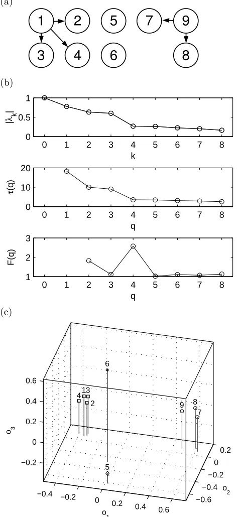
The coupling coefficientsǫij were chosen from{0,1}to im-plement the coupling configuration depicted in Fig. 1 (a), such that oscillators #2–4 are unidirectionally driven by #1, oscil-lators #7 and 8 driven by #9, and #5 and 6 are uncoupled. These differential equations were numerically integrated us-ing a step size of∆t = 0.01, starting from randomly cho-sen initial conditions. After discarding an initial transient of 104data points, further4×104samples entered data process-ing. Instantaneous phasesφjmof oscillatorsjat time points
tm = (m−1) ∆t were determined from thez-components using the analytic signal approach after removal of the tem-poral mean, and bivariate synchronization strengthsRijwere computed.
(a)
(b)
0 1 2 3 4 5 6 7 8
0 0.5 1
|
λ k
|
k
0 1 2 3 4 5 6 7 8
0 10 20
τ
(q)
q
0 1 2 3 4 5 6 7 8
1 2 3
F(q)
q
(c)
−0.4 −0.2
0 0.2
0.4 0.6 −0.6
−0.4 −0.2
0 0.2 −0.2
0 0.2 0.4 0.6
o 2 7 8 9
o 1 5 6
2 3 1 4
[image:6.612.59.296.56.571.2]o3
FIG. 1: Application of the eigenvector space method to a system of nine partially coupled Lorenz oscillators. (a) Coupling configuration: The left group of four oscillators is driven by #1, the right group of three driven by #9, the remaining two are uncoupled. (b) Eigenval-uesλk, timescalesτ(q), and timescale separation factorsF(q). The
maximal separation factorF(4)indicates the presence of four clus-ters. (c) Positions attributed to oscillators in 3-dimensional eigen-vector space(o1, o2, o3). The clustering by the k-means algorithm
results in a cluster composed of oscillators #1–4 (), two
single-element clusters consisting in oscillators #5 (⋄) and #6 (∗), respec-tively, and a cluster composed of oscillators #7–9 (◦).
timescale separation factorsF(q). A gap in the eigenvalue spectrum between indicesk= 3and4translates into a max-imum timescale separation factor forq = 4, which recom-mends a search for four clusters in the eigenvector space for timescaleτ = 3.5. This 3-dimensional space is depicted in Fig. 1 (c), where the expected grouping into four clusters can be clearly recognized in the arrangement of elementsj with positions~o(j). These four clusters that correspond to the two groups of driven oscillators and the two uncoupled oscillators (each of which forms a single-element cluster) are easily iden-tified by the k-means algorithm. The results shown here were obtained usingζ= 0.01; alternative choices of0.1and0.001 yielded the same clustering.
III. PERFORMANCE
To assess the performance of the eigenvector space method introduced in this paper, we compare it with the previous ap-proach to synchronization cluster analysis based on spectral decomposition. For reference, we briefly recollect the impor-tant details.
The participation index method [26] is based on the eigen-value decomposition of the symmetric synchronization matrix
Ritself, into eigenvaluesηkandL2-normalized eigenvectors
vk. Each of the eigenvectors that belong to an eigenvalue
ηk > 1 is identified with a cluster, and a system element
j is attributed to that clusterk in which it participates most strongly, as determined via the participation index
Πjk=ηkvjk2 , (23)
wherevjkare the eigenvector components ofvk. The method performs quite well in many configurations, but it encounters problems when confronted with clusters of similar strength that are slightly synchronized to each other, which was demonstrated in Ref. [27] using a simulation.
Here we employ a refined version of that simulation to com-pare the two methods. We consider a system ofN = 32 os-cillators forming two clusters, and check whether the methods are able to detect this structure from the bivariate synchroniza-tion matrixRfor different degrees of inter-cluster synchrony
ρint. The cluster sizes are controlled via a parameterr, such that the first cluster comprises elementsj = 1. . . r, the
sec-ond(r+ 1). . . N.
To be able to time-efficiently perform a large number of simulation runs and to have precise control over the structure of the generated synchronization matrices, we do not imple-ment the system via a set of differential equations. Instead, our model is parametrized in terms of the population value of the bivariate synchronization index, Eq. (1),
ρij =|hexp [i (φi−φj)]i| (24)
(whereh·i denotes the expectation value), which is the first theoretical moment of the circular phase difference distribu-tion [31]. Fori, j within the same cluster ρij is fixed at a value ofρ1 = ρ2 = 0.8. For inter-cluster synchronization
6
(a) (b)
r
ρ int
10 20 30
0.1 0.2 0.3 0.4 0.5 0.6 0.7 0.8
r
ρ int
10 20 30
[image:7.612.65.293.51.252.2]0.1 0.2 0.3 0.4 0.5 0.6 0.7 0.8
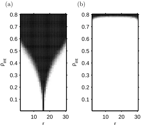
FIG. 2: Comparative performance of the participation index (a) and the eigenvector space method (b). The methods are tested on a sys-tem ofN = 32elements, divided into two clusters containingr
andN−relements, respectively. The inter-cluster synchronization strength ρintis varied from0 up to the value of intra-cluster
syn-chronization0.8. Synchronization matrices are generated based on samples of sizen = 200. The quantity shown is the relative fre-quency (over 100 trials) with which the respective algorithm failed to recover exactly the given two-cluster structure; it is visualized in gray scale, covering the range from 0 (white) to 1 (black). Compari-son shows that in a large area alongr = 16where the participation index method fails, the eigenvector space method introduced in this paper performs perfectly.
To be able to properly account for the effect of random vari-ations ofRijaroundρijdue to finite sample sizenwe gener-ated samples of phase values, using an extension of the single-cluster model introduced in Ref. [24]: The common behavior of oscillators within each of the two clusters is described by cluster phasesΦ1andΦ2. The phase differences between the
members of each cluster and the respective cluster phase,
∆φj=
φj−Φ1 forj= 1. . . r,
φj−Φ2 forj= (r+ 1). . . N, (25)
as well as the phase difference of the two cluster phases,
∆Φ = Φ2−Φ1, (26)
are assumed to be mutually independent random variables, distributed according to wrapped normal distributions [31] with circular momentsρ1C,ρ2C, andρCC, respectively. Since
the summation of independent circular random variables re-sults in the multiplication of their first moments [24], for the relation of model parameters and distribution moments holds
ρ1=ρ21C,
ρ2=ρ22C, (27)
ρint=ρ1CρCCρ2C.
For the performance comparison of the two methods,n= 200 realizations of this model of the multivariate distribution of
ρint
sample size n
0 0.2 0.4 0.6 0.8
50 100 150 200
FIG. 3: Performance of the eigenvector space method depending on the sample sizen, investigated using the two-cluster system of Fig. 2 for different values of the inter-cluster synchronization strengthρint.
The quantity shown here is the proportion of values of the parameter
r(controlling cluster sizes) at which the two-cluster structure failed to be recovered, visualized on a gray scale from 0 (white) to 1 (black). The plot shows that the ability of the eigenvector space method to correctly identify clusters up to high values ofρintbreaks down only
for very small sample sizesn.
phasesφj were generated for each setting of the parameters, and synchronization indicesRij were calculated via Eq. (1).
The clustering results are presented in Fig. 2 for the partic-ipation index and the eigenvector space method (usingζ = 0.01). The quantity shown is the relative frequency (over 100 instances of the matrixR) of the failure to identify correctly the two clusters built into the model. Figure 2 (a) shows that the participation index method fails systematically within a region located symmetrically aroundr=N/2 = 16(clusters of equal size). The region becomes wider for increasingρint but is already present for very small values of the inter-cluster synchronization strength. In contrast, the eigenvector space approach (b) is able to perfectly reconstruct the two clusters for all values ofrup to very strong inter-cluster synchroniza-tion. It fails to correctly recover the structure underlying the simulation data only in that region where inter-cluster syn-chronization indices attain values comparable to those within clusters, i.e., only where there are no longer two different clus-ters actually present. These results demonstrate that the eigen-vector space method is a clear improvement over the previous approach.
For real-world applications, a time series analysis method has to be able to work with a limited amount of data. In the case of synchronization cluster analysis, a small sample size attenuates the observed contrast between synchronization re-lations of different strength, making it harder to discern clus-ters. Using the two-cluster model described above, in a fur-ther simulation we investigated the effect of the sample size
10). For each value ofρintandn, as a test quantity the pro-portion ofr-values for which the algorithm did not correctly identify the two clusters was calculated. The result shown in Fig. 3 demonstrates that the performance of the eigenvector space method degrades only very slowly with decreasing sam-ple size. The method seems to be able to provide a meaningful clustering down to a data volume of aboutn= 30independent samples, making it quite robust against small sample size.
IV. CONCLUSION
We introduced a method for the identification of clusters of synchronized oscillators from multivariate time series. By translating the matrix of bivariate synchronization indicesR
into a stochastic matrix P describing a finite-state Markov process, we were able to utilize recent work on the coarse-graining of Markov chains via the eigenvalue decomposition ofP. Our method estimates the number of clusters present in the data based on the spectrum of eigenvalues, and it repre-sents the synchronization relations of oscillators by assigning to them positions in a low-dimensional space of eigenvectors,
thereby facilitating the identification of synchronization clus-ters. We showed that our approach does not suffer from the systematic errors made by a previous approach to synchro-nization cluster analysis based on eigenvalue decomposition, the participation index method. Finally, we demonstrated that the eigenvector space method is able to correctly identify clus-ters even given only a small amount of data. This robustness against small sample size makes it a promising candidate for field applications, where data availability is often an issue. Concluding we want to remark that though the method was de-scribed and assessed in this paper within the context of phase synchronization analysis, our approach might also give use-ful results when applied to other bivariate measures of signal interdependence.
Acknowledgments
The authors would like to thank Harald Atmanspacher, Pe-ter beim Graben, Mar´ıa Herrojo Ruiz, Klaus Lehnertz, Chris-tian Rummel, and Jiˇr´ı Wackermann for comments and discus-sions.
[1] M. S. Santhanam and P. K. Patra, Phys. Rev. E 64, 016102 (2001).
[2] N. Marwan, M. Thiel, and N. R. Nowaczyk, Nonlinear Proc. Geoph. 9, 325 (2002).
[3] V. Plerou, P. Gopikrishnan, B. Rosenow, L. A. N. Amaral, and H. E. Stanley, Phys. Rev. Lett. 83, 1471 (1999).
[4] E. Pereda, R. Quian Quiroga, and J. Bhattacharya, Prog. Neu-robiol. 77, 1 (2005).
[5] C. Zhou, L. Zemanov´a, G. Zamora, C. C. Hilgetag, and J. Kurths, Phys. Rev. Lett. 97, 238103 (2006).
[6] D. Brillinger, Time Series: Data Analysis and Theory (Holden-Day, 1981).
[7] M. B. Priestley, Nonlinear and Non-Stationary Time Series
Analysis (Academic Press, 1988).
[8] J. S. Bendat and A. G. Piersol, Random Data Analysis and
Mea-surement Procedure (Wiley, 2000).
[9] S. M. Kay, Modern Spectral Estimation (Prentice-Hall, 1988). [10] A. Kraskov, H. St¨ogbauer, and P. Grassberger, Phys. Rev. E 69,
066138 (2004).
[11] A. S. Pikovsky, M. G. Rosenblum, and J. Kurths,
Synchroniza-tion. A Universal Concept in Nonlinear Sciences (Wiley, 2000).
[12] S. Boccaletti, J. Kurths, G. Osipov, D. L. Valladares, and C. S. Zhou, Phys. Rep. 366, 1 (2002).
[13] M. G. Rosenblum, A. S. Pikovsky, and J. Kurths, Phys. Rev. Lett. 76, 1804 (1996).
[14] P. Tass, M. G. Rosenblum, J. Weule, J. Kurths, A. Pikovsky, J. Volkmann, A. Schnitzler, and H.-J. Freund, Phys. Rev. Letters
81, 3291 (1998).
[15] J.-P. Lachaux, E. Rodriguez, J. Martinerie, and F. J. Varela, Hum. Brain Mapp. 8, 194 (1999).
[16] F. Mormann, K. Lehnertz, P. David, and C. E. Elger, Physica D
144, 358 (2000).
[17] C. Granger and M. Hatanaka, Spectral Analysis of Economic
Time Series (Princeton University, 1964).
[18] B. Schelter, M. Winterhalder, R. Dahlhaus, J. Kurths, and J. Timmer, Phys. Rev. Lett. 96, 208103 (2006).
[19] D.-H. Kim and H. Jeong, Phys. Rev. E 72, 046133 (2005). [20] E. Rodriguez, N. George, J.-P. Lachaux, J. Martinerie, B.
Re-nault, and F. J. Varela, Nature 397, 430 (1999).
[21] V. Plerou, P. Gopikrishnan, B. Rosenow, L. A. N. Amaral, T. Guhr, and H. E. Stanley, Phys. Rev. E 65, 066126 (2002). [22] A. Utsugi, K. Ino, and M. Oshikawa, Phys. Rev. E 70, 026110
(2004).
[23] M. M¨uller, G. Baier, A. Galka, U. Stephani, and H. Muhle, Phys. Rev. E 71, 046116 (2005).
[24] C. Allefeld and J. Kurths, Int. J. Bifurcat. Chaos 14, 417 (2004). [25] C. Allefeld, Int. J. Bifurcat. Chaos 16, 3705 (2006).
[26] C. Allefeld, M. M¨uller, and J. Kurths, Int. J. Bifurcat. Chaos 17 (2007, in press), arXiv:0706.3375v1.
[27] S. Bialonski and K. Lehnertz, Phys. Rev. E 74, 051909 (2006). [28] G. Froyland, Physica D 200, 205 (2005).
[29] B. Gaveau and L. S. Schulman, B. Sci. Math. 129, 631 (2005). [30] P. Deuflhard and M. Weber, Linear Algebra Appl. 398, 161
(2005).
[31] K. V. Mardia and P. E. Jupp, Directional Statistics (Wiley, 2000).
[32] D. Gabor, J. IEE Part III 93, 429 (1946).
[33] R. Carmona, W.-L. Hwang, and B. Torr´esani, Practical
Time-Frequency Analysis (Academic Press, 1998).
[34] S. P. Meyn and R. L. Tweedie, Markov chains and stochastic
stability (Springer, 1993).
[35] J. B. MacQueen, in Proceedings of 5th Berkeley Symposium on
Mathematical Statistics and Probability (1967), pp. 281–297.