Orbit control of high area-to-mass ratio spacecraft using electrochromic coating

ORBIT CONTROL OF HIGH AREA-TO-MASS RATIO

SPACECRAFT USING ELECTROCHROMIC COATING

Charlotte M. Lücking

Advanced Space Concepts Laboratory, University of Strathclyde, Glasgow, United Kingdom, [email protected]

Camilla Colombo*, Colin R. McInnes†

ABSTRACT

This paper presents a novel method for the orbit control of high area-to-mass ratio spacecraft, such as spacecraft-on-a-chip, future „smart dust‟ devices and inflatable spacecraft. By changing the reflectivity coefficient of an electrochromic coating of the spacecraft, the perturbing effect of solar radiation pressure (SRP) is exploited to enable long-lived orbits and to control formations, without the need for propellant consumption or active pointing. The spacecraft is coated with a thin film of an electrochromic material that changes its reflectivity coefficient when a small current is applied. The change of reflectance alters the fraction of the radiation pressure force that is transmitted to the satellite, and hence has a direct effect on the spacecraft orbit evolution. The orbital element space is analysed to identify orbits which can be stabilised with electrochromic orbit control. A closed-loop feedback control method using an artificial potential field approach is introduced to stabilise these otherwise unsteady orbits. The stability of this solution is analysed and verified through numerical simulation. Finally, a test case is simulated in which the control method is used to perform orbital manoeuvres for a spacecraft formation.

NOTATION a semi-major axis

A area receiving solar radiation

aSRP acceleration due to solar radiation pressure

α incident angle of the sun light c speed of light in vacuum cR coefficient of reflectivity

e eccentricity

ε specific orbital energy f true anomaly

fON/OFF true anomalies of reflectivity switches

FS energy flux density of the sun

m satellite mass

μ gravitational parameter p semilatus rectum

 angle between the perigee of an in-plane orbit and the direction of the sun light

r spacecraft orbit radius rperi radius of the perigee

rE radius of the Earth

s size parameter of stability sphere

* _{ASCL, University of Strathclyde, Glasgow, UK,} [email protected]

†

ASCL, University of Strathclyde, Glasgow, UK, [email protected]

NOMENCLATURE ASCL Advanced Space Concepts Laboratory EM electrochromic material

EOC Electrochromic Orbit Control MEMS micro-electromechanical system PSZ potentially stabilisable zone S/C spacecraft

SRP solar radiation pressure I. INTRODUCTION I.I Introduction

Recent advances in miniaturisation make the prospect of near-term micro-electromechanical system (MEMS)-scale satellite missions realistic, employing system devices of length-scale 0.1-10 mm. These spacecraft offer cheap manufacture and launch, and can thus be deployed in large numbers providing multiple perspectives and real-time global information. The orbits of such satellites are influenced significantly by surface force perturbations such as solar radiation pressure and aerodynamic drag due to their high area-to-mass ratio. Area-to-area-to-mass ratio grows quickly as the spacecraft length-scale shrinks.

becoming a space debris hazard and endangering other satellites because of their lack of de-orbiting capability and probable future deployment in large quantity swarms.

The aim of this paper is to exploit the otherwise disadvantageous effect of solar radiation pressure induced orbital perturbations as a means of orbit control utilising electrochromic materials (EM).

The control method introduced here is intended primarily for micro-scale satellites-on-a-chip that do not possess the physical size for conventional orbit control actuators such as thrusters and have a naturally high area-to-mass-ratio. However, larger satellites could also exploit these findings by employing a large lightweight inflatable balloon with an electrochromic coating.

The advantages of using a balloon instead of a flat solar sail are the simpler unfolding mechanisms that could be standardised more easily and the freedom from the strict attitude control requirements that come with solar sails.

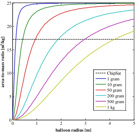
These so called “Satelloons” could have a main satellite bus as large a cubesat and would require balloons of up to 5m radius. Fig. 1 shows the area-to-mass ratio achievable with certain balloon radii for main bus satellites of different masses.

0 1 2 3 4 5

0 5 10 15 20 25

balloon radius [m]

a

r

e

a

-t

o

-m

a

ss

r

a

ti

o

[

m

2/k

g

]

ChipSat 1 gram 10 gram 50 gram 200 gram 500 gram 1 kg

Fig. 1: Area-to-mass ratio for "Satelloons" with a satellite module of different mass and a balloon of density 0.01 kg/m² for different balloon radii. Cornell University ChipSat1 (A/m = 17.2 m²/kg) in black and dashed as comparison.

The orbital dynamics of high area-to-mass ratio objects have been studied in the guise of planetary and interplanetary dust dynamics. Such motion is highly non-Keplerian due to the large influence of orbital

perturbations such as solar radiation pressure, aerodynamic drag, Poynting-Robertson drag, third body influences and electrostatic forces2-6.

Although there have been investigations directly into the dynamics of high area-to-mass-ratio spacecraft, these remained sparse until a recent surge of interest fuelled by increasing attention to the concept of solar sailing and advances in MEMS devices. Before this growing interest work on high area-to-mass ratio spacecraft stemmed from project Echo, an early experiment with reflective balloon satellites for passive terrestrial communications7. Later studies and simulations attempted to determine stable orbits and investigate novel astrodynamics occurring with these spacecraft, assuming them to behave completely passively8-12.

To actively control the influence of these perturbations was mainly the subject of solar sailing work, where a change in the attitude of the sail is used to direct the SRP effect on the spacecraft13, 14.

Micro-scale spacecraft pose a different challenge for orbit control because they are highly perturbed by SRP and not suitable for conventional orbit control methods. As the development of MEMS spacecraft advances the need for a simple and effective orbit control method grows. Recently, a number of projects to develop satellites-on-a-chip and “smart dust” devices have emerged1, 15-19. Proposed orbit control methods range from passive SRP control1 and Lorentz-force propulsion20 to spacecraft locally organised by Coulomb forces21.

The idea proposed in this paper is to alter the coefficient of reflectivity of a spacecraft by using electrochromic materials to control the spacecraft‟s orbit. These are materials that change their optical properties when a current is applied22. They are already widely used in terrestrial applications such as intelligent sunshades, tinting windows and flexible thin film displays23 and have been used in space applications, albeit not for orbit control. The recently launched IKAROS solar sailing demonstrator uses electrochromic surfaces on the sail to adjust its attitude24 and electrochromic radiators have been developed for thermal control25. A recent proposal to design the orbits of micro-particles by engineering their β-factor26 highlights the current interest in the exploitation of orbital perturbations as a means of trajectory manipulation of micro-scale artificial objects in space using simple control methods.

zone identified in section II as to whether and where stabilisation is possible. Section IV will use the results of the previous sections for a simulated case study in which the stabilisation control method is used for orbit manoeuvres of a spacecraft formation.

I.II Electrochromic Orbit Control

Electrochromic materials (EM) change their optical properties when a voltage or current is applied, thus modulating the fraction of light which is transmitted, absorbed and reflected, therefore effectively changing the reflectivity coefficient cR of the body. The effect

remains until a voltage or current in the opposite direction reverses it.

This paper proposes to use electrochromic spacecraft coatings to exploit the perturbing effect of solar radiation pressure for orbit stabilisation and manoeuvres. A spacecraft thus coated can change its coefficient of reflectivity between two set values. For a satellite-on-a-chip the minimum reflectance is 1, completely absorptive, because a lower value would mean that it were partially transmissive, and a maximum reflectance of 2. A balloon-type satellite, however, could turn translucent (cR = 0), allowing for a

larger modulation of the evolution of the orbit.

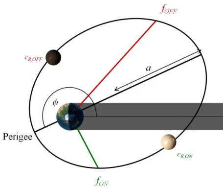
Fig. 2: Schematic of an electrochromically controlled orbit.

We consider a spacecraft on an Earth-centred orbit lying in the ecliptic plane, subject to solar radiation pressure (the effects of other perturbations are neglected). The orbit geometry, represented in Fig. 2, can be expressed through three in-plane orbital elements, semi-major axis a, eccentricity e, and the angular displacement between the orbit pericentre and the direction of the solar radiation through the centre of

the Earth . The acceleration any object receives from the solar radiation pressure (SRP) is given by:

2 cos ( )

S

SRP R

F A

a c

c m 

 

[1]

where cR is the coefficient of reflectivity, FS the

solar flux, c the speed of light, A the surface area receiving solar radiation, m the mass of the object and α the incident angle of the sun light. It can be seen that the value of a_SRP in Eq. [1] depends on the area-to-mass ratio of the object. Conventional spacecraft experience SRP only as a perturbing force whereas the effect on micro-scale satellites becomes dominant. Solar sailing technology exploits the acceleration due to solar radiation pressure by attaching a large light-weight reflective film to the satellite bus and controlling the thrust vector by varying the sail attitude (i.e. the angle α)13_{. Electrochromic orbit control (EOC) instead} modifies the reflectivity coefficient cR, with the

advantage that precise attitude control and complex sail deployment mechanisms are not necessary.

Because of the discrete nature of the reflectivity change, the orbit control has the characteristics of a bang-bang controller with the lower reflectivity state (cR,OFF) of the EM thin-film defined as the off-state and

the higher reflectivity state (cR,ON) as the on-state. It is

assumed that during each orbit the reflectivity can be switched twice. The true anomalies at which these changes take place are used as control parameters (fON

and fOFF in Fig. 2).

I.III Spacecraft Model

The spacecraft model considered in this paper is based on the Cornell University ChipSat concept 1. The spacecraft is a silicon microchip (density of 2330 kg/m3) of 1 cm2 area by 25 μm thickness and the area-to-mass ratio is 17.2 m2/kg. Because of its passive sun-pointing design a constant area-to-mass ratio is assumed so that α = 0º. The two values of reflectivity used in this paper are cR,OFF = 1 (completely absorptive) and cR,ON = 2

(completely reflective).

II. ORBIT STABILISATION II.I Control Potential

To analyse the usefulness of EOC for orbit stabilisation, firstly its control potential has to be assessed. This requires the maximum and minimum change in the Keplerian elements (Δa, Δe, Δ) achievable for any initial set of elements (a0, e0, 0) and

spacecraft parameters (A/m, cR,ON, cR,OFF) to be

determined.

The first step is to determine for each position (in true anomaly) on an orbit whether the change in the Keplerian elements (da/dt, de/dt, d/dt) is positive, negative or whether the spacecraft is in eclipse (and the orbital elements consequently remain constant since only SRP induced perturbations are considered).

Next, the maximum change in orbital element for a certain orbit can be determined by using cR,ON when the

change is positive to achieve the biggest possible effect and using cR,OFF when the change is negative to

minimise the negative effect. The minimum change can be obtained with the opposite strategy, using cR,ON when

the change is negative and cR,OFF when the change is

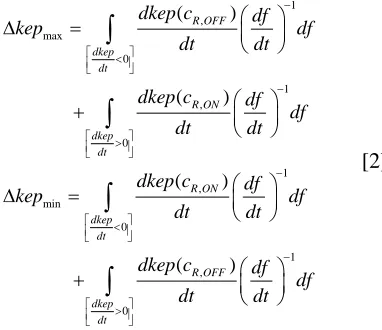
positive. The maximum and minimum change in orbital elements is computed through Eq. [2] where kep stands for any orbital element.

1 , max 0 1 , 0 1 , min 0 1 , 0 ( ) ( ) ( ) ( ) R OFF dkep dt R ON dkep dt R ON dkep dt R OFF dkep dt

dkep c df

kep df

dt dt

dkep c df

df

dt dt

dkep c df

kep df

dt dt

dkep c df

df dt dt   _       _       _       _         _{ }      _{ }       _{ }      _{ }  









[2]

dkep/dt is the variation of Keplerian elements, given by the Gauss‟ equations27, considering a disturbing acceleration given by Eq. [1], and df/dt is given by

2

2 ₂

(1 ) cos( ) ( ) sin( )

(1 )

r

a e p f a p r f a

df

dt r _{e a e}







  

 

 [3]

where a_r and a are the components of the SRP

acceleration in the radial and transversal directions in the orbital plane:









a a f

a_ a f

 

 

   [4]

The two integrals in each of the equations [2] are evaluated over the arc of a single orbit revolution 0 < f < 2π where dkep/dt is greater or smaller than zero.

The resulting map allows an assessment of possible points for stabilisation. These can only be orbits for which for all three in-plane elements the minimum change is negative and the maximum change is positive so that a zero net change is possible. This can be seen as a necessary criterion for stabilisation.

In the following subsections the control potential for all three in-plane orbital elements is analysed. Although only the results for a semi-major axis of 30,000 km are displayed in detail, the outcome for other semi-major axes is similar as will be shown in subsection II.V. II.II Semi-major Axis

The semi-major axis is directly related to the energy of an orbit. This relationship for elliptical orbits is described as:

2a



  

[5]

where μ is the gravitational parameter of the orbited planet in this case the Earth.

It can be seen that the specific orbital energy increases and decreases with the semi-major axis. When the solar radiation pressure is acting against the component of the spacecraft velocity vector that is in the direction of the sun light the spacecraft‟s kinetic energy is decreased. This means that the specific orbital energy is decreased and thus the change in semi-major axis is negative. The opposite is true when the SRP is acting in the direction of the spacecraft‟s velocity vector and the spacecraft is accelerated. The spacecraft orbital energy then increases and the change in semi-major axis is positive, so that27:

 





a e f a a

da r

dt _{a e}

   _       

[6]

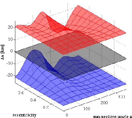
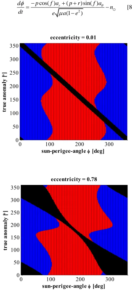
Fig. 3 shows the sign of da/dt as a function of the true anomaly along the orbit and the initial value of , for an initial semi-major axis of 30,000 km. Note that the sign of da/dt along a single orbit can be determined by covering a vertical line in Fig. 3, for a fixed value of

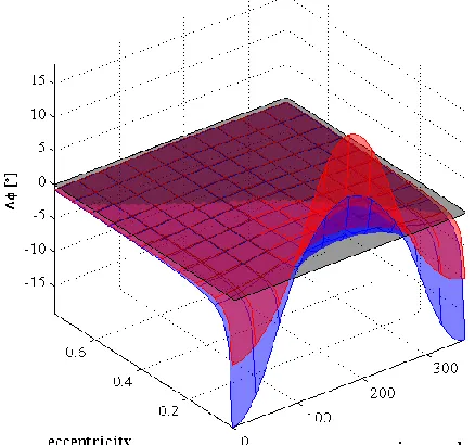
eccentricity 0.78 (the eccentricity at which the perigee lies in the Earth‟s lower atmosphere, without considering drag). For all orbits, positive and negative da/dt values exist. Fig. 4 shows the maximum and minimum change in semi-major axis achievable for all orbits with 30,000 km semi-major axis and eccentricity between 0.01 and 0.78 calculated with Eqs. [2] and [6]. The semi-transparent dark plane indicates a zero change of semi-major axis. It can be seen that at every point in the e--phase space this plane lies between the minimum and maximum change. Thus, a constant semi-major axis is always possible.

0 100 200 300

0 50 100 150 200 250 300 350

eccentricity = 0.01

sun-perigee-angle  [deg]

tr

ue

a

no

m

al

y

[



]

0 100 200 300

0 50 100 150 200 250 300 350

eccentricity = 0.78

sun-perigee-angle  [deg]

tr

ue

a

no

m

al

y

[



]

Fig. 3(a,b): Zones of positive (red), negative (blue) and zero (black) da/dt for orbits of different initial  with eccentricities 0.01 (a, top) and 0.78 (b, bottom) and 30,000 km semi-major axis. Zero da/dt zones are due to eclipses.

Fig. 4: maximum (red) and minimum (blue) change in semi-major axis for different orbits in the e--phase space portraying the floor and the ceiling of possible control options.

II.III Eccentricity

The variation of eccentricity is given by the Gauss equation27:

2

sin( ) [( ) cos( ) ] (1 )

r

p f a p r f re a

de

dt _{a e}





  



 [7]

0 100 200 300 0

50 100 150 200 250 300 350

eccentricity = 0.01

sun-perigee-angle  [deg]

tr

ue

a

no

m

al

y

[



]

0 100 200 300

0 50 100 150 200 250 300 350

eccentricity = 0.78

sun-perigee-angle  [deg]

tr

ue

a

no

m

al

y

[



]

Fig. 6(a, b): Zones of positive (red), negative (blue) and zero (black) de/dt for orbits of different initial  with eccentricities 0.01 (a, top) and 0.78 (b, bottom) and 30,000 km semi-major axis. Zero de/dt zones are due to eclipses.

Fig. 6 shows the sign of de/dt for a nearly circular and a highly-eccentric orbit. It can be seen that only small areas exist in which negative and postive change is experienced during one orbit (i.e., a vertical line in Fig. 6 with a fixed value of ) around = 0º and = 180º. These are consequently the only areas in which a positive Δemax and a negative Δemin can be found to stabilise the spacecraft. Fig. 5 shows the minimum and maximum Δe achievable for the spacecraft considered; the narrow gap between the two layers around zero at

= 0º and = 180º reflects the control potential in eccentricity limited to these regions.

II.IV Sun-Perigee Angle

The determination of the areas of positive or negative d/dt is also not trivial and it is described by the in-plane Gauss‟ equation for the change of the argument of perigee27 as:

2 cos( ) ( ) sin( )

(1 )

r

p f a p r f a

d

n

dt _{e a e}







  

 

  [8]

0 100 200 300

0 50 100 150 200 250 300 350

eccentricity = 0.01

sun-perigee-angle  [deg]

tr

ue

a

no

m

al

y

[



]

0 100 200 300

0 50 100 150 200 250 300 350

eccentricity = 0.78

sun-perigee-angle  [deg]

tr

ue

a

no

m

al

y

[



]

Fig. 7 shows the sign of d/dt for a quasi-circular and a highly-eccentric orbit as a function of the sun-perigee angle. It appears similar to the results of the eccentricity, albeit phase shifted. The significant difference is the fact that there is also a fixed rate of change in  due to the Earth‟s motion around the sun, n. In order to fix the orbit geometry, the SRP needs to

counteract this natural progression of . This leads to a zone where a stabilisation in  is possible that is not only found around = 90º and = 270º but in a halfmoon shape around = 180º. Fig. 8 shows the ceiling and floor of possible Δ values for different positions in the phase space.

Fig. 8: maximum (red) and minimum (blue) change in sun-perigee angle for different orbits in the e- -phase space portraying the floor and the ceiling of possible control options.

II.V The Potentially Stabilisable Zone (PSZ)

The results in sections II.II-IV can be combined to find possible points in the eccentricty and sun-perigee angle phase space where stabilisation is possible. To assess an orbit‟s usefulness for stabilisation of the three orbital elements considered, a new parameter is introduced. Skep is the lower value of the positive

Δkepmax and the negative Δkepmin. If this value is

negative the point is not useful for stabilisation because zero change is not within the range of possible control options, then Skep becomes zero, such that:

max min max min

max min

min({ , }) , if min({ , }) 0

0 , if min({ , }) 0

kep

kep kep kep kep

S

kep kep

    



  

 



[9]

Fig. 9 contains the results for all possible in-plane orbits with a semi-major axis of 30,000 km. The thick red line indicates the eccentricity above which the radius of the perigee is smaller than the radius of the Earth, rE. Only orbits below this line are possible. Sa is

portrayed in red contour lines since the semi-major axis can always be kept constant using EOC (see Section II.II) all positions in the phase space are acceptable for stabilisation when only considering this parameter.

The regions in which Se > 0, and thus the

eccentricity can be kept constant, are highlighted in blue. Additionally unmarked darker blue contour lines trace the Se values. As expected, these areas are thin

stripes around = 0º and = 180º (see Section II.III). The region in which S > 0 is highlighted in green. Additionally, unmarked darker green contour lines trace the S values. The resulting shape resembles a half moon with the highest S values towards the centre of the form.

Complete stabilisation is only possible in regions where all Skep values are larger than zero. This is

possible in a near rectangular shape with approx. 175° <

 < 185° and 0.15 < e < 0.3 named the potentially stabilisable zone (PSZ). This area is highlighted in bright cyan with a thick black border.

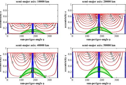
Figure 10 shows the same diagram for different semi-major axes. It can be seen that the width of the eccentricity zones is similar as is the shape of the sun-perigee-angle zone. The latter grows in eccentricity with increasing semi-major axis. This means that the PSZ size also increases in eccentrcity. The passively stable point identified by McInnes et al.28 for GEOSAIL, a solar sail investigating the Earth‟s geomagnetic tail, lies with the PSZ.

Fig. 11 shows the range in eccentricity of the PSZ for the spacecraft parameters given in I.III and varying semi-major axes. The rise in eccentricity and the extension of the range of the stable zone can be seen.

Fig. 12 contains information of the distance of the boundary of the PSZ from = 180° at the lower and upper eccentricity boundaries portrayed in Fig. 11. For the spacecraft data used in this simulation both values do not vary significantly from ~4° and even decrease slightly with increasing semi-major axis.

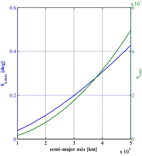
Finally, the maximum values for the control potential parameter Skep can be seen in

Fig. 13 and

Fig. 14. All three grow with increasing semi-major axis. The maximum Sa is at e ~ 0, the maximum Se can

4 4

6 6

8 8

10

10 10 10

12 12 12 12

14

14

14 14

14

14

16

16

16

16

16

16

18

18 18

18 ₁₈

18 18

18 20

20

20

20 20 20

20

20

20 20

sun-perigee-angle 

ec

ce

nt

ri

ci

ty

e

semi-major axis: 30000 km

0 50 100 150 200 250 300 350

0 0.1 0.2 0.3 0.4 0.5 0.6 0.7 0.8 0.9 1

Fig. 9: Sa (red) Se (blue) and S (green) for 30,000 km orbits in the e--phase space. Thick red line indicates where rperi = rE. The zone where the necessary criterion for stabilisation is fulfilled (PSZ) is marked in cyan with thick

black border.

0.2 0.2

0.3 0.3

0.4 0.4

0

.5 ₀.5 0.5 ₀.5

0

.6 0.6 0_.6 0.6

0

.7

0.7 0.7

0

.7

sun-perigee-angle 

ec

ce

nt

ri

ci

ty

e

semi-major axis: 10000 km

0 100 200 300

0 0.2 0.4 0.6 0.8 1

1 1

1.5₂ 1.5₂

2.5₃ 2.5₃

3.5₄ 3.54

4

.5 ₄.5 4_{.5 4}.5

5 5 5 5

5

.5 5

.5

5

.5 5

.5

6

6

6

6

6

sun-perigee-angle 

ec

ce

nt

ri

ci

ty

e

semi-major axis: 20000 km

0 100 200 300

0 0.2 0.4 0.6 0.8 1

15 15

20 20

25 ₂₅

30 30

35 35

40

40 40 40

45 45 45 45

50

50

50

50

50

sun-perigee-angle 

ec

ce

nt

ri

ci

ty

e

semi-major axis: 40000 km

0 100 200 300

0 0.2 0.4 0.6 0.8 1

30 30

40 40

50 50

60 ₆₀

70 70

80

80 80 80

90 90 90 90

sun-perigee-angle 

ec

ce

nt

ri

ci

ty

e

semi-major axis: 50000 km

0 100 200 300

0 0.2 0.4 0.6 0.8 1

Fig 10: Sa (red) Se (blue) and S (green) for orbits with different semi-major axes in the e--phase space.

1 2 3 4 5

x 104

0 0.05 0.1 0.15 0.2 0.25 0.3 0.35 0.4

semi-major axis [km]

ec

ce

nt

ri

ci

ty

lower boundary upper boundary

Fig. 11: The eccentricity value of the lower (blue) and upper (green) boundary of the PSZ at = 180° for different semi-major axes.

1 2 3 4 5

x 104

0 0.5 1 1.5 2 2.5 3 3.5 4 4.5 5

semi-major axis [km]



|



1

80

 |

lower boundary upper boundary

Fig. 12: The positive and negative distance of the boundary value for  from 180° at the lower (blue) and upper (green) eccentricity boundary of the PSZ for different semi-major axes.

1 2 3 4 5

x 104

0 10 20 30 40 50 60 70 80 90 100

semi-major axis [km] S a,m

ax

[

km

]

Fig. 13: maximum values of control potential parameter Sa for different semi-major axes.

1 2 3 4 5

x 104

0 0.2 0.4 0.6

semi-major axis [km]

S ,m

ax

[

de

g]

1 2 3 4 5

x 104

0 2 4 6

x 10-4

Se,m

ax

III. STABILISATION CONTROL METHOD III.I Controller Design

In section II.V the area in the phase space that fulfils the necessary criterion for stabilisation (PSZ) has been identified. The next step is to determine which of these orbits can be stabilised using electrochromic orbit control.

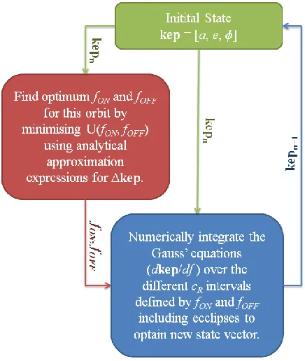
Fig. 15: Control loop for the simulation.

Fig. 15 shows the principle of the control loop. The control loop operates in discrete time steps of one orbit. Firstly, the initial orbit state is defined. Then the optimum control parameters (fON and fOFF) are

determined. Finally, the next orbit state is determined exactly using the numerical integration of the full dynamic model and the loop begins again.

The optimum control parameters are found with the following method: Initially the orbital elements at the end of a single orbit revolution for different sets of (fON, fOFF) are estimated using a set of analytical

equations which describe the secular variation of orbital elements due to SRP 29. The analytical approach is quicker than the computationally more expensive numerical integration of the full dynamical model, which would be impractical because of the large amounts of data sets examined.

Next, the values of a control function U(fON, fOFF) are

calculated. A search for the local minimum of

U(fON, fOFF) delivers the optimum control parameters fON

and fOFF. The control function is based on an artificial

potential field approach in the orbital element space. The desired position

































2 0

2 0

2 0

, ,

, ,

ON OFF a ON OFF

e ON OFF

ON OFF

U f f k a f f a

k e f f e

k_  f f 

 

 

 

[10]

where ka, ke and k are weight parameters, whose

value was expressed as function of the control potential parameter defined.

Fig. 13 shows the maximum values for Skep as an

indicator of the magnitude of the maximum step size in orbital elements over one orbit within the PSZ. The smaller this step size the more important it is to restrict the orbital element. The parameters kkep are defined as:

 

1 max

kep

kep

k

S



[11]

so that kkep









, 1

ON OFF

kep f f kep  , if the distance

between actual and desired position kep f





After the optimum set of control parameters has been determined, the orbit is then propagated through the numerical integration of the Gauss equations [6-8], employing the electrochromic orbit control and switching reflectivity at the chosen positions.

Because the analytical expressions used to predict the variation of Keplerian elements only consider the secular rate of change and neglect the periodic variation29, the predicted variation of elements is not exactly equal to the variation computed through numerical integration of the full model. This is not an issue, however, because it can be compared to the actual conditions in orbit where errors due to neglected perturbations also deliver results different from prediction. This shows that the control method is robust enough to deal with these uncertainties.

III.II Stability Conditions

The dimensions of the sphere around the position to be tested for stability are directly related to the control function. As defined in the previous subsection the part of the control function corresponding to any orbital element is equal to 1 when the distance between the actual position and the required position equals max(Skep). It is reasonable to size the sphere as a

multiple of this distance by a factor s, the size parameter of the stability sphere.

This factor can be chosen almost at random because if the position is unstable then the spacecraft will eventually exit the sphere however large it is as long as it is not big enough to distort the result by enclosing a different position that is indeed stable. Likewise, if the position is stable the spacecraft will stay within the sphere as long as it is not small enough to exclude positions around the initial state that the spacecraft may jump to and from while staying close to the desired position.

It is, however, desirable to have a sphere as small as possible to reduce the simulation time until a conclusion about stability can be drawn. A few trial simulations have shown that s = 1 is a reasonable figure with stability being assumed if the spacecraft does not exit the sphere for at least 100 orbits (approx. 60 days) for a semi-major axis of 30,000 km.

0-9 10-19 20-29 30-39 40-49 50-59 60-69 70-79 80-89 90-99 100+ 0

10 20 30 40 50 60 70 80 90 100

destabilising time [orbits]

p

er

ce

n

ta

g

e

o

f

p

o

in

ts

i

n

s

ta

b

il

it

y

z

o

n

e

uncontrolled SpaceChip controlled SpaceChip

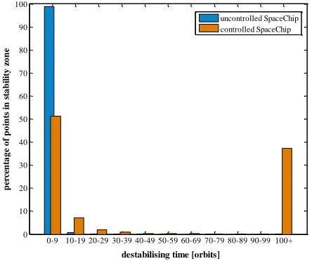
Fig. 16: Percentage of orbits in PSZ with certain destabilising times.

Fig. 16 shows the percentage of points in the PSZ that destabilise according to these criteria within certain times (measured in the number of orbits) for controlled and uncontrolled spacecraft. It can be seen that the vast majority of uncontrolled points destabilise within ten orbits (~99%). The other regimes have far smaller percentages but there are at least some points that last for longer than one hundred orbits.

For the uncontrolled spacecraft approximately one third of points are stable. The unstable ones destabilise

mostly within ten orbits. The sharp drop in points when looking at larger destabilising times suggest that the third defined as stable would not destabilise with just over one hundred orbits, but remain within the stability sphere indefinitely. Thus, both the size of the sphere and the maximum time of propagation are shown to be adequate.

III.III Simulation Results

The results of the simulation highlight the significant difference between the destabilising times of controlled and uncontrolled ChipSats. Fig. 17 visualises the results for both cases at 30,000 km semi-major axis. The uncontrolled ChipSat destabilises typically within ten orbits apart from an equilibrium point at = 180° and e ~ 0.22. Around this point the destabilising times become longer but the rise is very steep as can also be seen in Fig. 16 and Fig. 19. This is the stable point for the GEOSAIL mission28.

In contrast, the controlled ChipSats have a large area (approximately one third of the PSZ) in which the orbital lifetime exceeds one hundred orbits. Around the edges of this shape the destabilising time decreases rapidly so that half of the PSZ destabilises within ten orbits. The sudden increase in lifetime can also be seen in Fig. 19.

It is interesting to note that the semi-major axis rarely exceeded more than 10% of its allowed deviation in both the controlled and uncontrolled case. If an orbit is unstable it is always due to high deviations in e,  or both. Fig. 18 visualises the relation between  and e when the ChipSat exits the stability sphere.

The pattern for the uncontrolled ChipSat is very regular. Along = 180°  is the unstable parameter and horizontally along the eccentricity of the equilibrium point e is the unstable parameter. Between these two directions the transition between the parameters is smooth resulting in a circular domain.

The controlled spacecraft‟s pattern appears less smooth. In the upper and lower quarter of the diagram it appears similar to the uncontrolled case. In the middle, however, it results in a chaotic looking pattern. This can be explained with the randomness in the position of the spacecraft when leaving the sphere. To optimise the control the position will jump back and forth between positions favouring the eccentricity and those favouring

, thus moving in a zigzag path from the starting point. The moment the ChipSat leaves the sphere can be at either position.

LÜCKING ET AL.: ORBIT CONTROL OF HIGH AREA-TO-MASS RATIO SPACECRAFT USING ELECTROCHROMIC COATING  [] e c c e n tr ic it y e uncontrolled SpaceChip

176 178 180 182 184

0.16 0.18 0.2 0.22 0.24 0.26 0.28  [] e c c e n tr ic it y e controlled SpaceChip

176 178 180 182 184

0.16 0.18 0.2 0.22 0.24 0.26 0.28 d e st a b il is in g t im e [ o r b it s] 10 20 30 40 50 60 70 80 90 100+

Fig. 17: stability profile in PSZ for an uncontrolled/controlled ChipSat

 [] e c c e n tr ic it y e uncontrolled SpaceChip

176 178 180 182 184

0.16 0.18 0.2 0.22 0.24 0.26 0.28

176 178 180 182 184

0.16 0.18 0.2 0.22 0.24 0.26 0.28  [] e c c e n tr ic it y e controlled SpaceChip p a ra m e te r o u t o f b o u n d s

parameter out of bounds parameter out of bounds parameter out of bounds

parameter out of bounds MyStr3 p a ra m e te r o u t o f b o u n d s p a r a m e te r o u t o f b o u n d s d e st a b il isi n g t im e [ phi phi & e e

176 178 180 182 184 0

10 20 30 40 50 60 70 80 90

 []

d

e

st

a

b

il

is

in

g

t

im

e

[

o

r

b

it

s]

e=0.15 c. e=0.15 u. e=0.19 c. e=0.19 u. e=0.22 c. e=0.22 u. e=0.26 c. e=0.26 u. e=0.30 c. e=0.30 u.

Fig. 19: stability profile over  in PSZ for an uncontrolled (u., dashed) /controlled (c., solid) spacecraft and different eccentricities

IV. ORBIT MANOEUVRES IV.I Scenario

To demonstrate the effectiveness of the electrochromic orbit control method described in this paper a test case has been devised and simulated. A formation of eight ChipSats that originally shared the same orbit drifted apart in the phase space. They now occupy eight orbits with the same initial semi-major axis but differing in eccentricity and  so that they are located at the edges of the PSZ. The spacecraft have to be returned to the initial orbit using only electrochromic orbit control. Their relative spacing within the orbit is not considered.

Fig. 20: Locations of the spacecraft orbits before the manoeuvres.

The desired semi-major axis a0 was chosen to be

30,000 km and the desired eccentricity and sun-perigee-angle were selected to be close to the uncontrolled equilibrium orbit for these semi-major axis and spacecraft specifications: e0 = 0.22 and 0 = 180°. Fig.

20 shows the locations of the spacecraft orbits before the correction manoeuvre. The initial semi-major axes of the eight spacecraft are a0. The initial eccentricities

and -angles are located equally spaced on a ring around the desired orbit in the e--phase space with the maximum distance in each element corresponding to the dimensions of the PSZ (see Fig. 11 and Fig. 12). Table 1 contains the initial orbital elements of the spacecraft.

S/C No. e  [°] a [km]

1 0.220 184.0 30,000

2 0.262 182.8 30,000

3 0.280 180.0 30,000

4 0.262 177.2 30,000

5 0.220 176.0 30,000

6 0.178 177.2 30,000

7 0.160 180.0 30,000

8 0.178 182.8 30,000

Table 1: Initial orbital elements of spacecraft formation. IV.II Results

All eight spacecraft are eventually to be collected into the desired final orbit. There are, however, significant differences in the time required for the manoeuvre. Since the expansion of the PSZ relative to the maximum step size (approximated by Skep in

Fig. 13) is much smaller in  than in e, it is expected that the orbits of the two spacecraft with the initial positions of e = e0 , spacecraft no. 1 and no. 5, were the

first to be successfully corrected. It required 28 and 70 orbits respectively which is less than 17 and 42 days (orbit period is 14.36 hours at a semi-major axis of 30,000 km). All other spacecraft took considerably longer for their manoeuvres. Table 2 contains the results of the simulation displaying the manoeuvre duration for each of the spacecraft.

S/C No. Correction Time [orbits]

Approx. Correction Time [days]

1 28 16.8

2 935 559.4

3 541 323.7

4 638 381.7

5 70 41.9

6 546 326.7

7 745 445.8

8 538 321.9

Fig. 21 displays the orbits‟ progression of eccentricity and  in the phase plane. Fig. 22 shows the evolution of the orbital elements over time. It can be seen that the semi-major axes which were at the desired value to begin with diverge from it to enable the correction of the other elements due to the quadratic control function defined in Eq. [10]. The correction of the eccentricity proceeds almost linearly.

174 176 178 180 182 184 186

0.15 0.2 0.25 0.3

 []

e

c

c

e

n

tr

ic

it

y

S/C 4

S/C 5

S/C 6

S/C 7

S/C 8

S/C 1 S/C 2

S/C 3

Fig. 21: Evolution of the spacecraft‟s orbits in the e- -phase space.

The spacecraft that require large eccentricity manoeuvres at  ≈ 180° require the longest time to reach the desired position. Spacecraft number 2 requires 559.4 days. This can be explained with Fig. 5. Although much larger changes in eccentricity are possible in the rest of the phase space the potential Δe at 0° and 180° is very small. Yet this is the only region where a positive as well as a negative change is possible. To explore the possibilities for optimising the control of manoeuvres by exploiting these currents in the phase space outside the PSZ is subject of future work.

V. CONCLUSIONS

It has been shown that there is a region of orbits in the e- phase space in which high area-to-mass ratio spacecraft can be stabilised and manoeuvred using electrochromic coating. A simple quadratic penalty function based controller suffices to achieve this. High area-to-mass ratio spacecraft are usually micro-scale satellites-on-a-chip. However, larger spacecraft could also benefit from this technique by employing a large lightweight balloon covered in electrochromic material.

ACKNOWLEDGEMENTS

This work was funded by the European Research Council project VISIONSPACE (227571).

0

100

200

300

400

500

600

700

800

900

2.95

3

3.05

x 10

4

a

[

k

m

]

0

100

200

300

400

500

600

700

800

900

0.2

e

0

100

200

300

400

500

600

700

800

900

175

180

185

orbits



[



]

REFERENCES

1 _{Atchison, J.A. and Peck, M.A., A passive,}

sun-pointing, millimeter-scale solar sail. Acta

Astronautica 67 (1-2), 2009.

2 _{Gor'kavyi, N.N., Ozernoy, L.M. and Mather, J.C.,} A New Approach to Dynamical Evolution of

Interplanetary Dust. Astrophysical Journal 474

(1), 1997.

3 _{Greenberg, R. and Brahic, A., Planetary rings.} University of Arizona Press, Tucson, 1984. 4 _{Grotta-Ragazzo, C., Kulesza, M. and Salomao,}

P.A.S., Equatorial dynamics of charged particles

in planetary magnetospheres. Physica D:

Nonlinear Phenomena 225 (2), 2007.

5 _{Hamilton, D.P. and Krivov, A.V.,} Circumplanetary Dust Dynamics: Effects of Solar

Gravity, Radiation Pressure, Planetary

Oblateness, and Electromagnetism. Icarus 123

(2), 1996. 6

Howard, J.E., Horanyi, M. and Stewart, G.R., Global Dynamics of Charged Dust Particles in Planetary Magnetospheres. Physical Review Letters 83 (20), 1999.

7

Jakes, J.W.C., Project Echo. Bell Laboratories, New York, NY, United States, 1961.

8 _{Shapiro, I.I. and Jones, H.M., Perturbations of the}

Orbit of the Echo Balloon. Science 132 (3438),

1960.

9 _{Vilhena de Moraes, R., Solar radiation pressure} and balloon type artificial satellites. Presented at the Satellite Dynamics, Sao Paulo, Brazil, 1975. 10

Aksnes, K., Short-period and long-period perturbations of a spherical satellite due to direct

solar radiation. Celestial Mechanics and

Dynamical Astronomy 13 (1), 1976.

11 _{Harwood, N.M. and Swinerd, G.G., Long-periodic} and secular perturbations to the orbit of a spherical satellite due to direct solar radiation pressure. Celestial Mechanics and Dynamical Astronomy 62 (1), 1995.

12 _{Krivov, A.V. and Getino, J., Orbital evolution of} high-altitude balloon satellites. Astronomy and Astrophysics 318, 1997.

13

McInnes, C.R., Solar sailing: technology, dynamics and mission applications. Springer-Verlag, Berlin, 1999.

14

Wright, J.L., Space Sailing. Gordon and Breach Science Publishers, Amsterdam, 1993.

15 _{Barnhart, D.J., Vladimirova, T. and Sweeting,} M.N., Very-small-satellite design for distributed space missions. Journal of Spacecraft and Rockets 44 (6), 2007.

16 _{Sailor, M.J. and Link, J.R., "Smart dust":} nanostructured devices in a grain of sand. Chemical Communications (11), 2005.

17

Vladimirova, T., Xiaofeng, W. and Bridges, C.P., Development of a Satellite Sensor Network for Future Space Missions. Presented at the Aerospace Conference, 2008 IEEE, 2008. 18

Warneke, B., Last, M., Liebowitz, B. and Pister, K.S.J., Smart Dust: communicating with a cubic-millimeter computer. Computer 34 (1), 2001. 19 _{Warneke, B.A. and Pister, K.S.J., MEMS for}

distributed wireless sensor networks. Presented at the 9th International Conference on Electronics, Circuits and Systems, 2002.

20 _{Atchison, J.A. and Peck, M., A millimeter-scale} lorentz-propelled spacecraft. Hilton Head, SC, United states, 2007.

21 _{Schaub, H., Parker, G.G. and King, L.B.,} Challenges and prospects of Coulomb spacecraft formation control. Presented at the John L.Junkins Astrodynamics Symposium, 2004.

22 _{Monk, P.S., Mortimer, R.J. and Rosseinsky, D.R.,}

Electrochromism: Fundamentals and

Applications. Weinheim, New York, 1995. 23 _{Granqvist, C.G., Avendano, E. and Azens, A.,}

Electrochromic coatings and devices: Survey of some recent advances. Presented at the 4th International Conference on Coating, Braunschweig, Germany, 2002.

24 _{Kawaguchi, J., Mimasu, Y., Mori, O., Funase, R.,} Yamamoto, T. and Tsuda, Y., IKAROS - Ready for lift-off as the world's first solar sail demonstration in interplanetary space. Presented at the 60th International Astronautical Congress, IAC 2009, Daejeon, Korea, 2009. IAC-09-D1.1.3 25

Demiryont, H. and Moorehead, D.,

Electrochromic emissivity modulator for

spacecraft thermal management. Solar Energy Materials and Solar Cells 93 (12), 2009.

26 _{De Juan Ovelar, M., Llorens, J.M., Yam, C.H. and} Izzo, D., Transport of Nanoparticles in the Interplanetary Medium. Presented at the 60th International Astronautical Congress, Daejeon, Republic of Korea, 2009.

27 _{Battin, R.H., An Introduction to the Mathematics} and Methods of Astrodynamics, Revised Edition ed. AIAA, Inc., Reston, Virginia, 1999.

28

McInnes, C.R., Macdonald, M., Angelopolous, V. and Alexander, D., GEOSAIL: Exploring the geomagnetic tail using a small solar sail. Journal of Spacecraft and Rockets 38 (4), 2001.

29

Colombo, C. and McInnes, C.R., Orbital

dynamics of Earth-orbiting ‘smart dust’