Investigation of mixed element hybrid grid-based CFD methods for rotorcraft flow analysis

(1)

Whitehouse, G.R. and Boschitsch, A.H. and Smith, M.J. and Lynch, C.E. and Brown, R.E. (2010)

Investigation of mixed element hybrid grid-based CFD methods for rotorcraft flow analysis. In: 66th

American Helicopter Society Annual Forum: Rising to New Heights in Vertical Lift Technology,

11-13 May 2010, Phoenix, Arizona, USA.

http://strathprints.strath.ac.uk/

27363

/

Strathprints is designed to allow users to access the research output of the University of

Strathclyde. Copyright © and Moral Rights for the papers on this site are retained by the

individual authors and/or other copyright owners. You may not engage in further

distribution of the material for any profitmaking activities or any commercial gain. You

may freely distribute both the url (

http://strathprints.strath.ac.uk

) and the content of this

paper for research or study, educational, or not-for-profit purposes without prior

permission or charge. You may freely distribute the url (

http://strathprints.strath.ac.uk

)

of the Strathprints website.

(2)

Investigation of Mixed Element Hybrid Grid-Based CFD Methods for

Rotorcraft Flow Analysis

Glen R. Whitehouse and Alexander H. Boschitsch

[email protected]@continuum-dynamics.com Continuum Dynamics, Inc.

Ewing, New Jersey, 08618, USA

Marilyn J. Smith and C. Eric Lynch

[email protected]@gatech.edu Daniel Guggenheim School of Aerospace Engineering Georgia Institute of Technology, Atlanta, GA 30332-0150, USA

and

Richard E. Brown

[email protected]

Department of Aerospace Engineering, University of Glasgow Glasgow, G12 8QQ, UK

Abstract

Accurate first-principles flow prediction is essential to the design and development of rotorcraft, and while current numerical analysis tools can, in theory, model the complete flow field, in practice the accuracy of these tools is limited by various inherent numerical deficiencies. An approach that combines the first-principles physical modeling capability of CFD schemes with the vortex preservation capabilities of Lagrangian vortex methods has been developed recently that controls the numerical diffusion of the rotor wake in a grid-based solver by employing a vorticity-velocity, rather than primitive variable, formulation. Coupling strategies, including variable exchange protocols are evaluated using several unstructured, structured, and Cartesian-grid Reynolds Averaged Navier-Stokes (RANS)/Euler CFD solvers. Results obtained with the hybrid grid-based solvers illustrate the capability of this hybrid method to resolve vortex-dominated flow fields with lower cell counts than pure RANS/Euler methods.

Nomenclature

*

C_T thrust coefficient

n iteration number

n unit surface normal vector

q flow state

R rotor radius

R coordinate vector

S surface

S vorticity source term

t time

u velocity field

u∞ free stream velocity field

V volume

ν viscosity

ρ air density

ρ source point coordinate vector

Presented at the American Helicopter Society 66th

ω vorticity vector

Ω rotor rotation rate

Ω coupling interface region

Introduction

Accurately determining the fluid dynamic environment is critical to the calculation of rotorcraft performance. Since the helical wake usually remains near the rotor blades for an appreciable amount of time, inaccurate or diffusive wake modeling also leads to poor predictions of blade loading and BVI events so that correct prediction of the wake strength, structure and position is essential. Both Lagrangian vortex methods and grid-based Computational Fluid Dynamics (CFD) techniques have been developed to numerically simulate rotor wake flows; however, while such analysis tools are capable of predicting the loading on rotors under various flight conditions, formulational assumptions or computational cost constrain their routine application to general configurations.

(3)

are limited in their ability to address viscous and compressible flow. While extensions of these methods can address compressibility and viscous effects to a limited degree, only Navier-Stokes CFD solvers are capable of reproducing all of the significant fluid dynamics mechanisms and producing predictions of sufficient engineering accuracy for both steady and unsteady blade loading [1-3].

Lagrangian free-wake methods, where the rotor wake is modeled as a vortex filament (or a collection of vortex filaments) trailed from each blade, can predict adequately the wake induced loading on a rotor for a variety of flight conditions and applications [4-11]. Such methods offer fast turnaround times, even real-time, and can be easily coupled to lifting-line and panel methods. While these approaches are ideally suited to propagating vortices over long distances and offer a compact flow description, their efficiency deteriorates for flight conditions where the rotor wake undergoes large scale distortions (e.g. strong wake on wake interactions such as vortex ring state, airframe interactions, and ground effect). In such situations, the neglected viscous and compressibility effects are likely to become significant. Also, core distortions become pronounced and must be modeled empirically.

Traditional grid-based CFD methods (i.e., solution of the density, velocity and pressure variables), do not make any a-priori assumptions about the shape and evolution of the flow-field. These techniques are, in principle, capable of modeling the formation, evolution, coalescence and rupture of the complete rotor wake. Unfortunately, because of the helical/epicycloidal nature of the rotor wake, regions of strong vorticity remain near to the rotor for appreciable amounts of time, and the extended action of numerical diffusion, inherent in current differencing methods can quickly smear the vorticity without expensive grid refinement [12].

The ability to preserve intense vortices and other localized flow features in rotorcraft flow-field calculations remains a major challenge, and many researchers have tried to solve the numerical diffusion-induced problem, with limited success, by increasing both the grid resolution and the accuracy of the numerical technique used to transfer flow properties from one grid cell to the next [13-20]. Vorticity Confinement [21-25] can also be added to the CFD formulation, but results are highly sensitive to parameter settings [23].

Attempts have also been made to combine the best features of CFD and vortex filament techniques [26-35] and whilst these coupled solutions generally yield improved performance predictions for a select number of flight conditions, they still suffer from numerical diffusion of the rotor wake, particularly near the blade

tip in the region where the wake has not rolled up sufficiently to start the Lagrangian solution [26, 36-38]. In addition, these techniques have difficulty modeling flight regimes where vortices pass close to the rotor blade [28, 35, 39].

Lagrangian particle methods have also been coupled to CFD tools to address the diffusion of vorticity [40, 41]. These methods typically suffer from the same limitations as their filament based counterparts, which is expected since vortex particles are functionally

equivalent to very short filament segments.

Furthermore, while particle methods have been very successful at solving two-dimensional problems, difficulties associated with maintaining divergence-free vorticity fields and managing particle disorder [42], preclude routine application of such methods to high Reynolds number three-dimensional flows, such as those associated with rotorcraft. Nevertheless, promising research in this area based on rotor blade beam/lifting line models is ongoing [43, 44].

Recently, it has been shown that numerical diffusion of the rotor wake can be controlled in a CFD solver – albeit, one based on a vorticity-velocity formulation – by carefully constructing the flux formula and selecting an appropriate flux limiter [45-47]. The Vorticity Transport Model (VTM), however, has not been developed to the extent where it can provide good a-priori predictions of blade aerodynamics, and is driven by a Weissinger-L panel method coupled to airfoil data tables. This limitation motivated the development of a modular flow solver, VorTran-M, initially based on the CFD solver in VTM that can be coupled to a conventional Navier-Stokes code [48, 49]. In this arrangement, the Navier-Stokes solver is used to resolve the (presumably small) regions of compressible viscous flow near to the blades, and VorTran-M is applied to the remaining, vortex dominated flow domain. Such an arrangement simultaneously exploits the ability of traditional CFD to predict local aerodynamics and the low dissipation first principles wake modeling capabilities of VorTran-M in the wake.

Building upon the prior work presented in [48-50], this paper explores concepts for accurate hybrid coupling and presents results from the integration of a velocity-vorticity solver, VorTran-M with several unstructured, structured and Cartesian based RANS/Euler CFD solvers.

Vorticity Transport Methodology

(4)

associated vorticity distribution, ω=∇×u, then for

incompressible 3D flow this equation is stated as follows:

S

u

t

+

⋅

∇

−

⋅

∇

=

∇

+

∂

_ω

_υ

2

_ω

(1)

where S is a vorticity source representing vorticity that arises on solid surfaces immersed in the flow. For rotary wing aircraft, the wake arises as a vorticity source associated with the aerodynamic loading of the rotor blades, fuselage, wings, and other parts of the vehicle. The velocity induced by this vorticity distribution at any point in space is governed by the Biot-Savart relationship,

ω

×

−∇

=

∇

2

u

(2)

that, when coupled to Equation 1, feeds back the strength and geometry of the rotor wake to the loading of the rotor blades and fuselage.

VorTran-M employs a direct numerical solution to Equations 1 and 2 to calculate the evolution of the rotor wake. At the beginning of each time step the numerical implementation calculates the velocity, u, at which the vorticity field must be advected, by inverting Equation 2 with either cyclic reduction [45, 51, 52] or a Cartesian Fast Multipole method on an adaptive grid [46, 53, 54]. The vorticity distribution is then advanced through time using a discretized version of Equation 1, obtained using Toro’s Weighted Average Flux (WAF) algorithm [55] and Strang spatial splitting. This process is then repeated for each time step.

This numerical technique conserves vorticity explicitly, and has been shown to preserve the vortical structures of rotor wakes for very long times. Numerical diffusion still admits the spreading of vorticity, but this can be controlled by implementing a suitable flux limiter in the WAF scheme [56]. Such an approach is in contrast to that of [57], where a vorticity-velocity formulation is employed to conserve vorticity, however use of conventional flux limiters results in the same large cell counts (30 across a vortex) as traditional CFD to resolve vortical flow fields.

Figure 1, demonstrates the ability of this formulation to capture detail in the wake structure of a hovering rotor even with a relatively coarse grid (800,000 grid cells, 50 cells per rotor radius, 6 cells per blade chord) [49]. This example illustrates that if the vortical structures in the wake are accurately resolved, then the solution will

show experimentally observed fluid dynamic

[image:4.612.349.507.73.211.2]

phenomena such as the growth of the vortex pairing instability and the subsequent loss of symmetry in the wake downstream of the rotor.

Figure 1: Snapshot of vortex paring in the wake beneath a two bladed hovering rotor from [53]

Computational Fluid Dynamic Solvers

An important goal of the work presented here is to demonstrate the feasibility of successfully and efficiently implementing a hybrid arrangement in a variety of CFD solvers and to identify and address key numerical issues arising from the interface treatment. Thus, the development of a hybrid CFD/VorTran-M solver has been investigated using four distinct CFD methodologies: CDI’s RSA3D (unstructured RANS) and CGE (Cartesian grid Euler) codes, as well as NASA’s OVERFLOW (structured overset RANS) and FUN3D (unstructured RANS).

RSA3D

CDI’s Rotor Stator Analysis in 3D (RSA3D) was originally developed under the sponsorship of NASA Glenn Research Center to model aeroelastic rotor-stator interaction problems, and can also analyze flows over

propellers, rotors, complex multistage

compressors/turbines and cascades [58-61]. RSA3D solves the RANS equations on a unstructured moving deforming grid using multigrid acceleration strategies [58]. It also includes an efficient quad-tree-based interpolation scheme to handle the sliding rotor-stator interface in a consistent and conservative manner, as

well as an optional containment-dual based

discretization scheme to reduce dissipation on high aspect ratio grids [59-61].

CGE

(5)

Cartesian mesh does not need to be boundary conforming. Moreover, while primarily intended to solve compressible flows, CGE has also been shown to behave well for low speed flows with Mach number less than 0.1.

OVERFLOW

NASA’s OVERFLOW (2.1) code [63-65] solves the compressible RANS equations on either single block or Chimera overset mesh systems for all types of grid topologies (O-, H- C-). Second-order temporal integration is achieved via dual time stepping or Newton sub-iterations. Spatial discretization options include a range of schemes from second to fifth order accuracy. Low-Mach number preconditioning is available to compute low-speed flows.

FUN3D

The FUN3D code has been developed at the NASA Langley Research Center [66-68] to solve both compressible and incompressible RANS equations on unstructured tetrahedral or mixed element meshes. The incompressible RANS equations are simulated via Chorin's artificial compressibility method [69]. A first-order backward Euler scheme with local time stepping is applied for steady-state simulations, while a second-order backward differentiation formula (BDF) resolves time-accurate simulations. Non-overlapping control volumes surround each cell vertex or node where the flow variables are stored, resulting in a node-based solution scheme. An overset mesh capability resolves multiple frames of motion within one simulation [70].

Hybrid Grid-Based CFD Solver Development

General and versatile interfacing strategies for coupling

CFD methods to a vorticity-velocity (ω-u) based solver

have been developed that build upon commonly used techniques for coupling numerical flow solvers together, and incorporate new elements to account for grid motion and support the immersion of multiple bodies (rotor blades, rotors and/or fuselage components) in the flow.

The coupling strategy relies on the VorTran-M module for vorticity transport outside of the CFD domain and utilizes the CFD solver to handle the viscous compressible flow near the surfaces and provide the vorticity source terms requires in VorTran-M.

The coupling procedure is guided by several considerations regarding the underlying formulations and capabilities of the respective codes:

1. In order to control numerical dissipation within

the CFD solver at minimal cost, it is desirable to use a fine mesh over the smallest volume

necessary. However, since ω-u formulations are

usually incompressible, the CFD grid must extend sufficiently far that the effects of compressibility outside the domain can be neglected.

2. In a vorticity-velocity formulation, the velocity

anywhere inside a domain is completely determined by the vorticity distribution over the domain and the velocity distribution over the domain boundary.

3. In general, the CFD grid will move relative to the

mesh used by the ω-u method.

4. The local flow solution is transferred from the

CFD solver to the ω-u solver where it is then

evolved according to the vorticity transport equation. Steps must be taken to prevent double counting of vorticity by ensuring that once the

vorticity is transferred to the ω-u solver, it or its

evolved derivative will not be projected again at a later time step.

CFD/ωωωω−−−−u Coupling Strategies

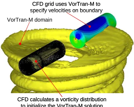
Coupling CFD to vorticity-velocity methods requires a two-way interface (see Figure 2), which has been implemented using both direct coupling, where the CFD code calls the vorticity-velocity solver as a compiled library, and also using Python-based strategies. Several methods have been employed for hybrid coupling, and the following paragraphs review these methods and present their advantages and limitations in the context of the current application.

CFD grid uses VorTran-M to specify velocities on boundary

VorTran-M domain

CFD calculates a vorticity distribution to initialize the VorTran-M solution

CFD grid uses VorTran-M to specify velocities on boundary

VorTran-M domain

CFD calculates a vorticity distribution to initialize the VorTran-M solution

Figure 2: Schematic of multi-domain CFD/VorTran-M coupling

Initializing the Wake Vorticity

Loading approach: By far the most common method for

[image:5.612.319.533.443.613.2]

(6)

circulation, and hence vorticity, in the wake [33, 35, 71]. In its simplest form the peak circulation is used to set the strength of a single vortex filament located either at the blade tip, location of peak circulation or at the centroid of circulation. More sophisticated adaptations trail multiple filaments from the blade based on the change in circulation along the span. Such an approach is relatively simple and robust and builds upon the assumption that the CFD predicted loading should provide the most accurate representation of the near wake. Unfortunately, this strategy implicitly uses a thin-wake assumption (i.e. a Kutta condition is applied so that the wake leaves the trailing edge of the blade) [33] where any vorticity related to separated flow is accounted for in terms of changes in the strength of the wake, but NOT the location (relative to the leading and trailing edges). An additional concern with this method is that without care in providing wake feedback on the CFD solution, it is possible for the near field representation to diverge from the free-wake since the CFD method and the wake approach solve different equations (i.e. viscous and compressible CFD verses incompressible inviscid free wake).

Direct coupling: Direct (volumetric and boundary)

coupling approaches can also be employed to initialize the wake by setting the three components of vorticity based on the vorticity in each CFD cell on the cells at the outer boundary of the CFD domain (i.e. the CFD domain is discretized as one particle per CFD cell, or one filament per CFD cell). For particle methods [40, 41], care must be taken to ensure that there is sufficient CFD resolution to maintain adequate particle overlap, however for filament based approaches the situation becomes more complicated. A single filament can be trailed from each CFD boundary face based on the circulation in each cell, however determining the shed component and the filament connectivity is complicated and may result in a very inefficient wake representation (i.e. many weak filaments). Of course, some alternate representation of the vorticity interior to the boundary must be included for correct evaluation of the Biot-Savart equation. A more sophisticated application of this method is employed in the VTM code [46] and by Zhao and He [44] where the loading (albeit from a lifting line/surface style thin wake) is projected onto a temporally and spatially changing interpolation surface prior to discretization.

Providing Feedback to the CFD Solver

Boundary coupling: The simplest way to provide

feedback to the CFD solver is via modifications to the outer boundary state [39, 40]. This ensures that the tip vortex trajectories predicted by the wake and CFD solvers align at the boundary. Unfortunately, this approach requires adequate resolution in the CFD domain to ensure adequate resolution to the tip vortex,

as well as sophisticated boundary conditions to prevent the spurious reflections from the interface [39].

Perturbation Approach: This approach attempts to

decouple the flow field (i.e. the Navier-Stokes/Euler equations) into a rapidly varying vortical component that can be solved separately with a suitable wake model, and a smoothly varying part that can be accurately solved using a CFD solver that captures effects neglected by the wake model [31, 32]. Though conceptually appealing, this approach breaks down when, due to its own modeling idealizations, the wake model “drifts” from the true solution and so no longer provides a useful reference solution from which the smoothly varying part can be developed. More generally, decoupling the solution to the Navier-Stokes/Euler equations is not always possible if there are solid bodies in the computational domain because the boundary conditions do not decouple conveniently. If the wake model relies upon a Biot-Savart law to calculate the wake-induced velocity, and velocities are required at every grid point in the CFD domain, then the perturbation approach can become prohibitively expensive for 3D computations even if some sort of field based method, such as Fast Multipole or Poisson equation inversion, is employed. A variation of this approach is employed in the HELIX code, where vortex embedding is used to drive a potential flow model [26, 29, 30]. Here the physical velocity components are decomposed into a part associated with the velocity potential and a vortical part associated with regions of the flow containing the rotor wake. A Lagrangian technique is employed to model the wake, and this wake solution is then embedded into the potential flow domain by interpolating the wake induced velocity from the Lagrangian wake into the appropriate cell in the potential domain [72, 73].

Surface Transpiration Approach: This approach directly

addresses the computational expense and generality of the perturbation approach by evaluating the rotor wake induced velocities only at those grid points that are located on surfaces immersed in the flow [74, 75]. In essence, this technique serves to implicitly alter the local angle of attack of each aerodynamic segment of along the rotor blade, and is only strictly valid for Euler calculations where no boundary layer is modeled and the velocity at the surface of the blade can be non-zero. Moreover, because the influence between the rotor wake and CFD models is essentially one-way (i.e. the wake model sets transpiration velocities in the CFD calculation, but the CFD flow solution usually has no bearing upon the wake model) the method remains limited in its ability to model the vortex distortions

resulting from vortex-vortex and vortex-surface

(7)

Field Velocity Approach: The field velocity approach

uses the techniques of indicial modeling to permit the influence of the rotor wake to alter the time metrics of the CFD grid without actually distorting the grid [28, 33, 35, 76, 77]. This is a quasi-steady type of approach that linearizes the induced velocity of the rotor wake, but neglects the effects of the wake pressure and density fields. While this technique inherently neglects second order wake effects, it is potentially more accurate than the surface transpiration method and less complex than the perturbation approach. However, like the surface transpiration approach, the field velocity technique attempts to address the boundary condition problems of the perturbation method by evaluating the rotor wake induced velocity on the surface of the rotor blade; unfortunately, this location, where the no-slip boundary condition should be enforced, is exactly where vorticity-based wake models have problems and poor predictions of the blade surface velocities may result. Additional problems may arise from double counting of the wake-induced velocity since both the CFD solver and the wake solver have solutions in the overlap region. A recent application of this approach has attempted to address this limitation by not including the induced velocity influence of the free wake in the overlap region when calculating the field velocities [33], unfortunately, given the definition of the Biot-Savart relationship, this strategy results in erroneous induced velocities.

Hybrid Approach: This technique is a hybrid pseudo

overset approach that couples multiple separate computational domains; an inner (CFD) and an outer (wake) domain, connected by an overlap region. The outer domain serves to set the boundary conditions of the inner domain, whilst the overlap region functions as an interpolation region to determine the passage of the flow from one domain to the other. This hybrid approach addresses the shortcomings of the approaches described above by evaluating the rotor wake induced velocities in an overlap region of the flow where both the CFD and wake methods provide adequate modeling fidelity. By suitably choosing the size and location of the overlap region, this technique can be made to preserve the spatial resolution of each numerical solver and thus maintain an accurate representation of the flow passing between the two domains. Furthermore, this approach minimizes computational cost associated with having two coupled solutions since the extra evaluation of the Biot-Savart relationship is required only at the intersection of the two domains rather than throughout the two complete numerical domains as in the perturbation and field velocity approaches. Since the majority of the wake is represented in the vorticity-velocity domain, this hybrid method further optimizes the use of computational resources since it is no longer necessary to devote tightly spaced grid points in the

far-field to preserve wake vortices. The inner CFD grid can thus now be limited to the small regions about the surfaces where compressibility and viscosity are important and high resolution of vortex-vortex and vortex-surface interactions is required.

In the hybrid coupling scheme, the wake solver vorticity in a selected region is overwritten with values from the CFD solution at every time step (see Figure 2). This procedure, described in detail in [49] eliminates double counting and also facilitates the handling of moving grids, a requirement for efficient rotorcraft modeling. While other options can be considered, the overwriting procedure appears to be the most effective in simultaneously accommodating general moving grids while retaining simplicity in both formulation and code implementation.

VorTran-M/CFD Coupling Strategy

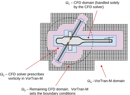
These considerations motivated the current approach for rotorcraft applications that defines four regions in the flow domain and treats vorticity differently in each domain. These regions, summarized in Figure 3, are defined as:

Ω1: Lies inside CFD boundaries, and encloses all

solid surfaces. The flow is represented entirely

by the CFD solver. Ω1, can be disjoint, as in

Figure 2, but must contain all solid bodies of interest.

Ω2: Surrounds Ω1 and lies inside CFD boundaries.

The flow is represented by CFD solver. The flow solution is transferred to VorTran-M at the start of every time step, thus overwriting the VorTran-M solution in this region. VorTran-VorTran-M evolves the vorticity during the time step to determine the

amount of vorticity that advects out of Ω2.

Ω3: Consists of the remaining CFD domain lying

outside of region Ω2. Both VorTran-M and the

CFD solver evolve the flow in the normal manner. This region is usually small, often only several cells thick, and promotes solution stability by preventing instantaneous feedback between the solvers. The VorTran-M module sets the outer CFD boundary conditions.

Ω4: Consists of the remaining VorTran-M domain

lying outside of region Ω3. The flow is entirely

represented by VorTran-M.

Time Stepping Strategy

A time stepping strategy is defined that consists of advancing both the CFD and vorticity-velocity solutions forward in time and then overwriting the

(8)

Ω1– CFD domain (handled solely by the CFD solver)

Ω2– CFD solver prescribes vorticity in VorTran-M

Ω3– Remaining CFD domain. VorTran-M sets the boundary conditions

Ω4–VorTran-M domain

Figure 3: Detailed schematic of CFD/VorTran-M overlap regions

At time

t

n, a solution in both the CFD and VorTran-M

domains is available. This solution is advanced to the

next time level,

t

n+1, using the respective integration

strategies. In most arrangements, an implicit time marching strategy is used in the CFD code where the discrete set of equations defining the flow field update,

n CFD n

CFD

q

+1

−

are evaluated at

t

n+1. Since VorTran-M

employs an explicit scheme it is most convenient to first

advance the VorTran-M solution to

t

n+1 so that the

resulting flow field,

ω

_VorTrann+1 ₋_M and

q

_VorTrann+1 ₋_M, are available to evaluate flow states at the CFD boundary. Once both the VorTran-M and CFD solvers have

advanced the solution to

t

n+1, the overwrite step is

performed where the CFD solution in Ω₂ (which may

differ from step to step) overwrites the VorTran-M solution.

Coupling Interfaces: General Cell Intersection

and Insertion

Application to Unstructured Grids

A direct cell intersection method (vorticity*volume) based on the coupling strategy described above was tested via a RSA3D and VorTran-M coupling. Here, the vorticity field in the region overlap region is calculated by finite differencing the CFD solver velocity field. RSA3D uses an unstructured grid vertex based scheme to interface with VorTran-M, thus the volume integrated vorticity in a tetrahedral cell is

∑

∫

=

×

≅

×

=

×

∇

=

4 1

3

1

k k k S V

S

u

dS

u

n

dV

u

α

(3)

where uk is the velocity at tetrahedral vertex, k, and Sk is the outward directed area of the face opposite node, k.

The last identity follows from the identity,

∑

S

_k

=

0

,

for closed polyhedra.

For inviscid calculations, the surface velocity, us, is nonzero. If one considers the inviscid result as the limiting case of a viscous calculation where the boundary layer has become infinitesimally thin, then it is clear that the boundary layer must contain vorticity in order to transition from zero velocity at the surface (no-slip condition) to us at an infinitesimal height above it. The vorticity strength associated with a surface area, A, is given by:

∫

∇

×

=

×

=

×

=

δ δ

γ

S A S V

S

u

dV

n

u

dS

n

u

dS

(4)

where V_δ is the infinitesimal volume occupied by the

vorticity sheet of thickness, δ, lying upon the area, A; S_δ

is the bounding surface of V_δ. For moving surfaces it is

also necessary to compute a “source” term:

∑

∫

=

×

≅

⋅

=

3 1

3

1

k k A

S

n

u

dS

A

u

β

(5)

Other than its inherent discrete approximations, the Biot-Savart relation provides a complete description of

the flow field provided that α and the surface velocities

are known.

A finite wing configuration, summarized in Table 1,

provided a useful first test for the hybrid

RSA3D/VorTran-M arrangement. Calculations were performed on different grids having identical chordwise resolution (128 mesh points about the airfoil), but varying outer boundary placements. The smallest grid extends only 1.5 chord lengths away from the blade surface, which by conventional CFD standards would be considered far too small for reliable results. The large grid is more typical and extends 10 chords away from the surface. In all cases, a smoothly varying mesh is obtained by constraining the grid spacing to grow no faster than by a factor of 1.1 from element to element. For the hybrid calculations, the finest VorTran-M mesh spacing is set to 2% span (18% chord) which is about twice the free-steam convection distance in a time step (i.e., CFL=0.5) thus ensuring a stable VorTran-M calculation using its explicit time marching method. The Courant numbers for the finest mesh cells on the CFD side are significantly greater than 1.0 and implicit time stepping is necessary in RSA3D.

The wing, at 8o angle of attack, is impulsively started

[image:8.612.80.295.73.231.2]

(9)

[image:9.612.343.509.100.241.2]

structures located near to the wing tips, see Figure 4. These vortex structures lower the lift coefficient in a time dependent manner. Inviscid, low Mach number flow and small flow angles are assumed thus allowing comparison to classical theories.

Table 1: Fixed wing parameters

Profile NACA 0012

Aspect Ratio (AR) 8.8

Mach Number (M_∞₎ _0.2

270K Cell Mesh x ∈ (-1.5c, +2.5c)

492K Cell Mesh x ∈ (-10.c, +11c)

Estimates for the 3D lift coefficient, CL3D=a3Dα for the

NACA 0012 airfoil in inviscid flow were drawn from several sources. The steady state 2D and 3D lift curve

slopes, a2D and a3D, are approximately (for non-elliptic

wings) connected by the aspect ratio according to:

(

τ

)

π





+









+

=

1

2

2 3

AR

a

D D

D (6)

where for the case presented here τ=0.2 [78]. XFOIL

[79] predicts, CL2D =0.9957 at M∞=0.2, which translates

to CL3D =0.7603. Inviscid calculations with the RSA3D

code using a fine grid extending 10 chords upstream and

downstream from the surface predict CL3D =0.7573,

[image:9.612.313.539.573.714.2]

which agrees closely (~0.4%) with the XFOIL prediction.

Figure 4 shows the developing wake structure obtained with the hybrid RSA3D/VorTran-M including the starting and trailing vortices. The most striking observation is the preservation of the starting vortex as it traverses the VorTran-M mesh. The ability to sustain this vortex poses a challenge for any Eulerian formulation because it varies rapidly in both space and time. The trailing vortex structures on the other hand also vary rapidly in space, but for this problem steady state conditions near the wing are achieved that do not exhibit significant temporal variation. The ability to resolve the starting vortex multiple spans downstream without significant dissipation attests to VorTran-M’s inherent strength when applied to vortex dominated flow problems. The CFD code on the other hand is unable to preserve this vortical structure because of numerical diffusion on this grid. Temporally growing wavy perturbations can be observed along the trailing

vortices suggesting an aerodynamic instability.

Twisting striations in the trailing filaments are also

evident and are consistent with the locally induced swirl.

Figure 4: Perspective view of the developing wake structure for an impulsively started wing. All iso-surfaces are drawn at the same vorticity magnitude.

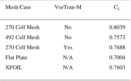
The steady state lift coefficients obtained with the various grids are summarized in Table 2 . The main observation from this table is that the use of the VorTran-M considerably improves the predicted lift coefficient for the reduced domain CFD meshes. For example, the lift predicted with the hybrid method on the small extent mesh (270,000 cells, outer boundaries located 1.5 chords from the surface) agrees with the large domain CFD and XFOIL predictions to within 1.1% error. Without the VorTran-M module to represent the flow outside the CFD domain, the error is 5.7%. Generally, the CFD predictions on the truncated mesh tend to overestimate the lift coefficient compared to the large mesh CFD results, and this is because truncating the wake eliminates the influence of the downstream wake, thus reducing the induced downwash and increasing the effective angle of attack. These results show that not only is the vorticity being correctly transferred from RSA3D to VorTran-M solutions, but the influence of this convecting wake is being fed back properly to the RSA3D solution via the outer boundary conditions.

Table 2: Computed steady state lift coefficients

Mesh/Case VorTran-M CL

270 Cell Mesh No 0.8039

492 Cell Mesh No 0.7573

270 Cell Mesh Yes 0.7688

Flat Plate N/A 0.7004

(10)

A bluff body wake is considered next. Unlike the relatively thin wakes shed from aerodynamically clean surfaces, bluff body type flows are dominated by unsteadiness and periodically shed vortical structures. Simulating such flows serves to demonstrate the hybrid code’s abilities to reliably predict the spatial and temporal structure of the wake.

The wake structure and characteristic shedding frequencies are strongly influenced by the feedback (in terms of induced velocities) of the wake upon the fixed surfaces. Reliable prediction of these structures therefore is contingent upon the accurate transmission of wake-induced velocities at the outer boundaries back to the body.

The bluff body simulations consisted of orienting the

wing described in Table 1 at 90o angle of attack and

impulsively starting the calculation with M_∞=0.2. The

RSA3D/VorTran-M calculation was carried out using the 270,000 tet. grid used earlier and a near grid VorTran-M spacing of 18% chord. While the grid would be too coarse for resolving features near the surface, it appears adequate for capturing the wake dynamics further downstream.

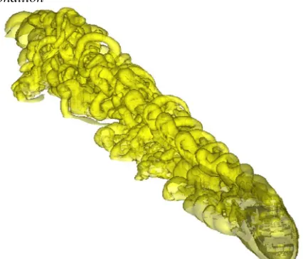
The wake after 1800 time steps, when the wake has convected approximately 67 chords downstream, is shown in Figure 5. By this point a periodic vortex shedding process is fully established with spanwise vortices of approximately equal and opposite vorticity being generated successively off the trailing and leading edges. The near wake exhibits intricate linking structure and strong three-dimensional features which are attributed to end-effects that must arise to enforce the Helmholtz constraint (i.e., vortices cannot terminate in the flow so that each of the strong spanwise vortices must link to one or more of its oppositely oriented neighbors via streamwise connecting vortices to form closed loops of vorticity). Further downstream, the vortex induced stretching and subsequent inter-linking results in finer scale structures. The numerous eddies tend to cancel each other so that their net far-field influence becomes small. This implies that in CFD calculations it is only necessary to resolve the nearest portions of the wake where the larger vortex structures dominate the wake-induced contributions back on the shedding body.

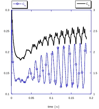
Sample force time histories are presented in Figure 6 below. The fluctuations are induced by the vortex street associated with periodic wake shedding that occurs as the flow passes the wing. The force history reflects the overall evolution of the flow beginning with formation of the starting vortex that then convects downstream while symmetry in the wake breaks thus leading to the three-dimensional vortex street.

Periodic spanwise shedding of vorticity forming characteristic vortex street

Side view

Top view

Periodic chordwise shedding of vorticity interacting with the quasi-2D vortex street

Figure 5: Wake geometry expressed as vorticity iso-surface for the rectangular wing positioned normal to the flow

0.1 0.15 0.2 0.25 0.3

1 1.5 2 2.5 3

0 0.05 0.1 0.15 0.2

C

N CD

[image:10.612.317.536.64.318.2]

time [ s ]

Figure 6: Force time histories for a wing at 90o angle of attack predicted by hybrid RSA3D VorTran-M code. Solid lines: lift coefficient, dashed lines: drag coefficient

A non-dimensional gauge of the vortex shedding frequency behind a bluff body is the Strouhal number,

V

fL

St

=

(7)

[image:10.612.344.506.356.534.2]

(11)

edges; (ii) the evolution of the shed vortex wake geometry and (iii) the influence of the shed wake back upon the shedding body. For flow over a wing oriented perpendicular to the flow, the Strouhal number should be St=0.2 [80].

The force history shown in Figure 6 exhibits a periodic behavior with characteristic frequency f=71.4Hz which corresponds to a Strouhal number of St=0.2003. The drag response contains higher harmonics which is not surprising in light of the multiple 3D structures seen in

Figure 5. The lift (normal force, CN) response is

dominated by the first harmonic and contains a bias away from zero due to asymmetry (the NACA 0012 airfoil is not symmetric about the mid-chord plane).

The hybrid RSA3D/VorTran-M code is thus able to reproduce the oscillatory response at close to the expected frequency using a coarse, limited-extent mesh and a small fraction of the computational resources required for a pure CFD computation.

Unlike the fixed wing calculations above, rotorcraft flow fields pose unique challenges for traditional CFD solvers because the wake retains its strength and remains near the rotor for long periods. Performing such calculations with RSA3D/VorTran-M serves to

illustrate the long-term vorticity preservation

capabilities of the model. Furthermore, the vorticity shed from a rotor can re-enter the CFD domain of the subsequent blade. This raises a new challenge for hybrid modeling, namely the ability to transmit re-entrant vorticity that convects from the outer VorTran-M domain into the CFD calculation across the CFD outer boundary.

Slow speed ascent and high speed forward flight

(µ=0.325) simulations were performed using a rotor

similar to the active elevon rotor experiments of Fulton [81], however, to expedite turnaround time a two-bladed (rather than the original four-bladed) version of the rotor was simulated. A VR-12 profile was adopted, which is freely accessible and similar to the VR-18 cross-section actually used in the test. The blade twist gradient was

10°/R. Each blade grid was generated by sweeping a

2D triangular grid along the span with 128 nodes about the chord and 16 intervals along the span. The root section (r=56.3 cm) is open and the mesh boundary on this section is treated as an outer boundary allowing both incoming and exiting relative flow. One consequence of this modeling approximation is that it suppresses the formation of a root vortex. The grid associated with each rotor blade contains 72,000 points and the grids are completely disconnected. Therefore all interactions and coupling between the blade flow fields must be effected through the vortical solution convected in VorTran-M. These calculations therefore

demonstrate both the moving mesh and multiple domain capabilities of the hybrid RSA3D VorTran-M code.

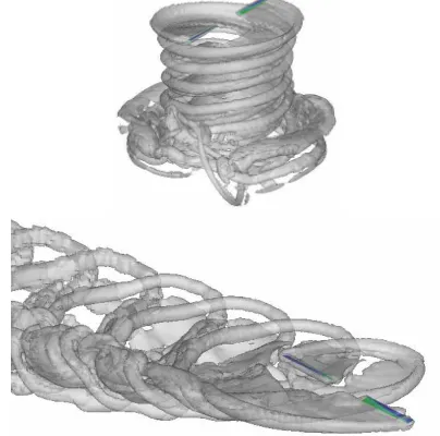
In each case shown in Figure 7 the rotation rate was 1070 RPM and no trimming of the rotor was attempted. The collective was fixed such that the tip angle of attack

in hover was 11°. Both predictions showed excellent

preservation of the rotor wake.

Figure 7: RSA3D/VorTran-M rotor wake predictions: two bladed untrimmed rotor in slow speed ascent (upper) and two bladed untrimmed rotor in forward flight (lower)

Application to Cartesian-Grids

The same direct vorticity*volume insertion method as with RSA3D, was evaluated in CGE/VorTran-M. Here cell intersection was trivial by enforcing exact alignment between the CGE and VorTran-M cells (see Figure 8).

The CGE/VorTran-M methodology resulted in the first commercial ship wake database for a real-time tactical flight simulator [62]. This effort, for the US Navy’s MH-60R/SH-60B tactical operational flight trainers, included over 192 ship/flow condition combinations,

with the wake flow field sampled at ≤1m spacing out to

4 ship lengths downstream.

Despite the limitations of the application of an Euler formulation near to the deck of the ship, predictions compared well with scale model and full scale ship airwake measurements (see [62] for more details). A sample ship airwake prediction is shown for a LPD-4 class ship in Figure 9 and exhibits a similar cascade in

vortical scales as the wing at 90o angle of attack

[image:11.612.323.525.174.374.2]

(12)

[image:12.612.77.294.68.263.2]

Figure 8: Intersection of Cartesian grid (red) and VorTran-M grid (green) at right for a yawed flow condition

Figure 9: CGE/VorTran-M prediction of a LPD-4 class ship airwake

Application to Structured Grids

Given the positive results obtained using the simple vorticity insertion method in the CGE/VorTran-M, a similar vorticity-based technique was examined [50] using the NASA OVERFLOW (2.1ab) structured overset solver.

Predictions for a single-bladed rotor configuration in forward flight are presented in Figure 10 through Figure 12. The rotor configuration consisted of a modified NACA 0012 airfoil section (O-grid with 91 x 89 x 31 cells) and two end caps (67 x 39 x 41 cells each). A body of revolution representing a rotor hub (71 x 121 x 37 cells) was also included in the analysis. To facilitate the vorticity-based coupling a non rotating outer rectangular grid domain (271 x 271 x 52 cubic cells

with ∆s≈0.22c) containing the entire rotor system was

used to calculate the vorticity required by VorTran-M.

Pure OVERFLOW results are presented that utilized an off-body grid system where the grid levels coarsened by a factor of two between the near-field of the rotor system to the far field region of the computational domain. For the hybrid OVERFLOW/VorTran-M case where the OVERFLOW outer near body grid was used to input the vorticity for VorTran-M, the finest cell size in the VorTran-M domain was then set to twice the size

of the near body grid (∆s≈0.43c) cell, and the

subsequent grid coarsening occurred at every rotor radius downstream.

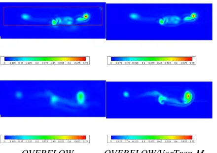
Results are presented in Figure 10 after 2550 time steps (~630 degrees) when the starting vortex has convected approximately one diameter downstream. Here, the extent of the OVERFLOW near body grids is outlined in red and the active VorTran-M grid in blue. On these grids, the pure OVERFLOW computation is normally dissipative in nature and hence unable to preserve significant vorticity in the rotor wake beyond approximately one rotor revolution. The coupled OVERFLOW/VorTran-M solution, on the other hand, is able to preserve the entire wake flow, including the starting vortex, see Figure 10.

OVERFLOW

OVERFLOW/VorTran-M

Figure 10: Predictions of wake vorticity, plotted at the same level of vorticity magnitude, for a 1-bladed rotor in forward flight after 2550 time steps

[image:12.612.79.292.295.477.2] [image:12.612.333.516.353.651.2]

(13)

speed of sound) for these two solutions is shown on the slices, perpendicular to the direction of flight, downstream of the rotor plane, in Figure 11 and Figure 12.

Figure 11 top compares the predictions on a slice 23.2 chord lengths aft of the rotor hub, and, despite the two-fold difference in cell size between the OVERFLOW near body grid (the red box in Figure 11 upper left) and VorTran-M, both show almost identical vorticity fields (peak vorticity for both cases is 0.77). Further downstream, 31.7 chords lengths (Figure 11 bottom), the solutions start to diverge with the OVERFLOW predicting a peak vorticity (0.36) that is half the OVERFLOW/VorTran-M value (0.72). By 33.3 chord lengths downstream (Figure 12 top), the VorTran-M grid for the hybrid calculation has been coarsened to twice the resolution of the corresponding OVERFLOW grid, yet the solution clearly demonstrates a high degree of the conservation of the peak vorticity. It is important to mention that the OVERFLOW solution has diffused the rotor blade tip vortex to a magnitude of 0.29 peak value, whereas the hybrid solver predicted a distinct core structure with peak of 0.79. Similar trends are shown at 40 chord lengths downstream in Figure 12

bottom

, where the OVERFLOW predicted peak

vorticity has been diffused to about 20% the value of the hybrid OVERFLOW/VorTran-M solution on a grid that is twice as coarse.

OVERFLOW OVERFLOW/VorTran-M

Figure 11: Predicted vorticity magnitude for a 1-bladed rotor in forward flight on a plane perpendicular to the direction of flight, 23.2 (upper) chord lengths and 31.7 (lower) downstream of the hub. ∆sOVERFLOW (red region

at left) ≈0.22c, ∆sOVERFLOW≈0.43c and ∆sVorTran-M≈0.43c

The OVERFLOW/VorTran-M coupling presented above uses simple vorticity injection to initialize the VorTran vorticity sources. This works well when the grids are nicely aligned, but very poorly when they are not due to interpolation errors. These errors can be remedied by using a fine CFD grid, surrounding all

bodies in the flow, but this option results in high (dominant) computational cost associated with this grid. Another option is to implement formal cell intersection routines, as with RSA3D; however such methods are complicated, invasive and expensive.

[image:13.612.318.537.146.307.2]

OVERFLOW OVERFLOW/VorTran-M

Figure 12: Predicted vorticity magnitude for a 1-bladed rotor in forward flight on a plane perpendicular to the direction of flight, 33 (upper) chord lengths and 40 (lower) downstream of the hub. ∆sOVERFLOW≈0.43c and

∆sVorTran-M≈0.87c

Coupling Interfaces: Velocity-Based Coupling

Method

Application to Structured Grids

To address these deficiencies a more general velocity-based coupling that builds upon the observations defining flows in terms of vorticity and velocity was developed. Here, the velocity, rather than vorticity, was passed from the CFD code to VorTran-M at the VorTran-M cell corners in the overlap region. Within VorTran-M, the vorticity field was calculated by appropriately finite differencing the velocity field. This procedure can be facilitated by setting up a near body grid in a structured mesh that is identical to the finest VorTran-M grid. When implemented for use with OVERFLOW, the OVERFLOW solver treats this grid like any other, and automatically performs grid motion and hole cutting as the blades rotate, flap and, in the case of aeroelastic calculations, deform. The VorTran-M interface then uses this information to account for VorTran-M cells that intersect the body using a modified version of method described in [82]. At the end of each time step VorTran-M sets the OVERFLOW grid boundary conditions at the outer edge of this grid, or on other grids in the solution.

Sample predictions from [50] for the 8o collective, 1250

[image:13.612.78.298.416.571.2]

(14)

81 cells with y+=0.955, tip and root caps 85 x 79 x 61 cells) and a body of revolution hub. The two bladed rotor was then surrounded by the VorTran-M grid with

cells of ∆s≈0.13c. VorTran-M set the boundary

conditions on an additional grid of cubic cells with

∆s≈0.13c (112 x 58 x 36 cells that rotates with and

encloses the rotor system, see Figure 13. After approximately 6000 time steps, this results in a total of 7.2 million active cells.

Figure 13: 2-bladed rotor and hub grid arrangement. Blade grids (black), tip-caps (blue), root-cap (red), hub grid (green), bounds of initial VorTran-M grid (blue line) and grid on which VorTran-M sets boundary conditions (red line)

A close up of the rotor wake in the near-body region

predicted with pure OVERFLOW† and with the coupled

OVERFLOW/VorTran-M is plotted in Figure 14, where OVERFLOW alone predicts very little root vorticity and significantly diffuses the tip vortices after about

ψ~135o. Conversely, OVERFLOW/VorTran-M

predicts significant loading along the entire span of the blade, with the tip vortices cleanly exiting the near-body region. The lack of inboard vorticity predicted by OVERFLOW also manifests itself in the rotor thrust coefficient and blade loading shown in Figure 15. OVERFLOW predicts the magnitude of the loading near to the tip, but significantly underpredicts the loading inboard of 0.8R. The integrated thrust

coefficient for this case was CT=0.00432, or 94% of the

experimental value. OVERFLOW/VorTran-M more

accurately reproduces the thrust coefficient

(CT=0.00458, or 99.6% of the experimental value) and

the inboard loading. However, the 0.5R is still somewhat underpredicted, though this may be due to the relatively low number of revolutions simulated in these predictions. Nevertheless, the improved ability of OVERFLOW/VorTran-M to predict the spanwise

†_{Pure OVERFLOW predictions were undertaken on the}

same near-body grid arrangement as the hybrid OVERFLOW/VorTran-M. Automatic off-body grid generation was used with a factor of 2 spacing that resulted in a grid with 19.8 million cells.

loading for this hovering rotor configuration on this non-optimized relatively coarse grid is significant.

No blade root vorticity

Blade root vorticity

Figure 14: Close-up of OVERFLOW (upper) and OVERFLOW/VorTran-M (lower) predictions of the near-body wake and velocity vectors on a slice through the rotor from [50]

Predictions of the tip vortex trajectory are compared to experimental measurements in Figure 16 where the error bars represent the error associated with locating the center of the tip vortex (i.e. local grid cell size). Wake trajectory data was extracted from the pure

OVERFLOW prediction for the first 270o, after which

the predicted vorticity was insufficient to identify discrete vortices. Plotting Q-criterion may aid tip vortex identification, however all results presented here are based on iso-surface of vorticity magnitude.

0 0.05 0.1 0.15 0.2 0.25 0.3 0.35

0.2 0.3 0.4 0.5 0.6 0.7 0.8 0.9 1

r/R

CL

Caradonna & Tung OVERFLOW - 20K its OVERFLOW/VorTran-M - 6K its

Figure 15: Comparison of measured and predicted spanwise loading (CT Experiment = 0.0046, CT OVERFLOW =

[image:14.612.325.527.100.299.2] [image:14.612.98.274.188.314.2] [image:14.612.324.523.491.647.2]

(15)

0 0.05 0.1 0.15 0.2 0.25 0.3 0.35 0.4 0.45 0.5

0 50 100 150 200 250 300 350 400

Vortex Age (deg.)

V

o

rt

e

x

P

o

s

it

io

n

(

z

/R

)

0 0.1 0.2 0.3 0.4 0.5 0.6 0.7 0.8 0.9 1

V

o

rt

e

x

P

o

s

it

io

n

(

r/

R

)

Caradonna & Tung z/R OVERFLOW z/R OVERFLOW/VorTran-M z/R Caradonna & Tung r/R OVERFLOW r/R OVERFLOW/VorTran-M r/R

Figure 16: Comparison of measured and predicted tip vortex trajectory

Both solutions correctly predict the first 45o of tip

vortex evolution; for the next 180o, however

OVERFLOW predicts a tip vortex trajectory that is more outboard and lower than the measured data. Once significant wake interactions take place to distort the tip

vortices (after 180o tip vortices start to interact with the

next blade), OVERFLOW predicts a significant increase

in both the descent and contraction rates.

OVERFLOW/VorTran-M, correctly predicts the tip vortex trajectory for the entire revolution, with both the vertical and radial position of the wake closely tracking

the experimental data throughout.

OVERFLOW/VorTran-M also correctly predicts the asymptotic extent of radial contraction.

It should be noted, that in general the grids employed for the pure OVERFLOW calculation would be too coarse and non-optimal, by themselves, for reliable hover calculations. Consequently, the calculations presented here do no represent the best that OVERFLOW can do; rather they serve as a simple industrial scale baseline against which to compare the hybrid OVERFLOW/VorTran-M.

Application to Unstructured Grids

The preceding strategy was utilized to couple VorTran-M to NASA’s FUN3D code. Since the vorticity distribution is inferred from the velocities evaluated over a small sub-set of VorTran-M cells (those lying in

the overwrite region, Ω₂) all that is necessary is to

determine the FUN3D velocity at the cell corners of these VorTran-M cells.

Implementing such a velocity-based coupling requires that routines to interpolate velocities exist and that the surface definition (and/or suitable cell blanking information as in OVERFLOW) be made available to helper routines so that we can mark VorTran-M cells that are in the overlap region. Determining the FUN3D

velocity at the VorTran-M cell nodes can be performed efficiently (i.e. only one loop over the FUN3D grid). VorTran-M cells that have nodes inside the body can be made to take into account the bound vorticity (see [82] for more details). Similarly, since the overlap region can be defined in terms of VorTran-M cells, the VorTran-M nodes that are exterior to the FUN3D overlap region are not used.

Marking of the VorTran-M cells to calculate the overlap regions etc is performed at each time step. First the cells that intersect the surface are marked, and then based upon the desired size of the overlap and buffer region, cells are marked radially outwards away from the surface.

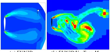
A sample FUN3D/VorTran-M prediction for the finite

wing at 90o angle of attack calculated using this strategy

is presented in Figure 17, along with pure FUN3D results on the same near-body grid. For this flow condition, the flow field is highly unsteady and dominated by vorticity shed and trailed from the leading and trailing edges of the wing. The flow field predicted by FUN3D (with a Spalart-Allmaras turbulence model) is shown in Figure 17 left, and exhibits separation from the upper and lower surfaces, with some wake shedding that is rapidly dissipated due to inadequate resolution in the downstream grid. In contrast, the hybrid FUN3D/VorTran-M prediction (Figure 17 right) using identical near-body mesh resolution shows a significant improvement in realism, comparable to RANS-LES predictions [84], with distinct vortices being shed from the surface, and propagated downstream.

(a) FUN3D (b) FUN3D/VorTran-M

Figure 17: Mid-plane vorticity magnitude predicted by the FUN3D/VorTran-M coupled simulation for the NACA0012 wing at 90o angle of attack

Lessons Learned

Three mixed element grid-based coupling interfaces have been implemented and assessed for various fixed, rotary and bluff-body configurations:

1. Cell intersection and insertion

2. Centroid-based vorticity*volume insertion

[image:15.612.79.293.72.238.2] [image:15.612.316.537.448.554.2]

(16)

In formal cell intersection, exact intersections of cubic VorTran-M cells and the CFD grid (for the cases presented here, the tetrahedra in an unstructured mesh see Figure 18 left), are developed and the intersection volume employed to transfer the vorticity calculated in each cell to the appropriate intersecting VorTran-M cells. Tests are also conducted to determine if the VorTran-M cells intersect the boundary or surface. This is necessary for Euler calculations to account for the “bound” vorticity associated with the surface slip velocity. Formal intersection is expensive, and requires extensive modification of the host CFD solver to determine the vorticity in each cell. Moreover, calculating the vorticity in the boundary layer (Figure 18 right), where a large fraction of the total CFD grid

resides, is a computational bottleneck‡. Despite this

computational cost and the required code modifications, results obtained with this method implemented within the constructs of RSA3D/VorTran-M were excellent.

Figure 18: Intersection of unstructured (blue) and VorTran-M grids (red) at left and center

To address these costs, a simplified approach was developed and tested out in the coupling of VorTran-M to the Cartesian grid solver CGE. Here, the

volume-weighted vorticity (i.e. vorticity*volume) was

calculated in overlapping cells and passed to VorTran-M at the cell centroid (see Figure 8). This method obviates the need for a formal intersection calculation since the grids coincide exactly (e.g., in the lower right portion of the red grid in Figure 8) and ensures conservation of the volume-integrated vorticity between the two codes. Again, surface bound vorticity is inserted into any intersecting cells. When coupled with the CGE, results were good.

Centroid-based vorticity insertion worked well for coupling to CGE and indeed certain OVERFLOW configurations because the CFD and VorTran-M grids can be made to align exactly and/or tight control can be placed on the size of the CFD cells in the overlap region. This is generally not the case for unstructured grids, or overset structured grids when the VorTran-M cell size approaches, or is smaller than that of the

‡

this is true of both velocity and vorticity-based

coupling and is controlled by the placement of Ω₂.

body grids and discontinuous vorticity distributions generally result.

A general coupling approach that eliminates these

complexities, computational costs and large

interpolation errors can be obtained by reformulating the coupling in terms of velocities evaluated at the vertices of a subset of the VorTran-M cells. This approach is efficient since resolution is now determined by the target VorTran-M mesh size. It is simpler since complex and invasive volume intersections are replaced by velocity interpolation procedures that are both simpler and often available in the host code. From Gauss’ integral theorem, the volume integral of the vorticity is directly related to the velocity integrated about the enclosing surface. From this result one can show that velocities at points that happen to lie inside a body evaluate to zero which produces consistent bound vorticity values. Finally significant cost savings, with no reduction in accuracy, can be attained by careful placement of the overlap regions.

Conclusions

This paper describes ongoing couplings between VorTran-M and several unstructured and structured grid Reynolds Averaged Navier-Stokes CFD solvers (CDI’s RSA3D, NASA’s OVERFLOW and FUN3D) and CDI’s CGE Cartesian grid solver with the goal of improving predictions of vorticity dominated flows by eliminating the diffusion issue that limits the application of pure Navier-Stokes/Euler solvers. Three coupling procedures have been described, along with sample results and lessons learned. The results presented here demonstrate improved wake and loading predictions.

Ongoing and Future Work

Work to date has focused on developing and demonstrating the feasibility a prototype hybrid CFD/VorTran-M flow solvers. Ongoing work seeks to improve the efficiency of the coupling in addition to further validation of the approach. It is anticipated that future work will investigate developing a parallel VorTran-M module, as well as refining the fundamental module coupling strategy to facilitate interfacing to a variety of CFD solvers.

Acknowledgements

[image:16.612.74.299.295.408.2]