Bak-Sneppen-type models and rank-driven processes

Bak–Sneppen type models and rank-driven processes

Michael Grinfeld,∗ Philip A. Knight,† and Andrew R. Wade‡ Department of Mathematics and Statistics

University of Strathclyde,

26 Richmond Street, Glasgow G1 1XH, UK

(Dated: August 1, 2011)

The Bak–Sneppen model is a well-known stochastic model of evolution that exhibits self-organized criticality; only a few analytical results have been established for it so far. We re-port a surprising connection between Bak–Sneppen type models and more tractable Markov processes that evolve without any reference to an underlying topology. Specifically, we show that in the case of a large number of species, the long time behaviour of the fitness profile in the Bak–Sneppen model can be replicated by a model with a purely rank-based update rule whose asymptotics can be studied rigorously.

PACS numbers: 02.50.Ga; 05.40.Fb; 05.65.+b; 87.23.Kg

Keywords: Bak–Sneppen model; thresholds; rank-driven Markov processes; self-organized

critical-ity; evolution

I. INTRODUCTION

In [1], Bak and Sneppen introduced a very fruitful and simple model of evolution that exhibits interesting dynamics but has proved surprisingly hard to analyse. The classical Bak–Sneppen (BS) model is a stochastic coarse-grained model of evolution of an ecosystem consisting of a fixed number N of evolutionary niches organised in a ring. Each niche is occupied by a species with a particular fitnessvalue in [0,1]. Direct inter-species interactions (predation, competition, etc.) occur only between species in neighbouring niches. The dynamics of the system is driven by the removal (extinction) of the least fit species in the entire system, whose niche is taken over by a new species; the extinction of the least fit species induces changes in the fitnesses of the species in the two neighbouring niches. In this contribution, we show we can algorithmically associate with the BS model a stochastic process whose update rule is defined solely in terms of theranks of the fitness values, without any reference to topology of interactions, which exhibits asymptotic behaviour and self-organized criticality statistics similar to those of the BS model.

We call processes of the type we associate to the BS model rank-driven processes (RDPs) and analyse them in detail in [2]. RDPs are of independent mathematical interest and can be used to define new evolution models.

In more detail, the BS model [1] is a discrete-time process which advances every time there is a species extinction event. Each species occupying the N niches is initially assigned a fitness

xk ∈ [0,1], k ∈ {1, . . . , N}, chosen independently from the uniform distribution on the unit interval, U[0,1]. At each step of the algorithm, we choose the smallest of all the xk, xkmin say, and replacexkmin and its two nearest neighboursxkmin±1 (indices calculated moduloN) by new

independentU[0,1]random numbers. In simulations with largeN, the marginal distribution of the fitness at any particular niche is seen to evolve to aU[s∗,1]distribution, withs∗ ≈0.667.

model [8] and so on.

A number of variants of Bak and Sneppen’s original model have been introduced which evolve according to different criteria. One simple variant is the discrete Bak-Sneppen model, in which fitnesses are only allowed to take the values0and1[9]; another is theanisotropicBak–Sneppen (aBS) model [10–12], in which, in addition to the least fit species, only its right-hand nearest neighbour is replaced. The aBS model also gives rise (according to large-N simulations) to a threshold value s∗ ≈ 0.724 [12]. Another variant on the BS model which eliminates topology is the mean-field version analysed in [13–15], in which one replaces the smallest fitness andK −1 randomly chosen other ones; below we show that such models fall within the RDP framework.

Rigorous results on the BS model include proofs the conjugacy of the discrete BS model to a contact process [16], of non-triviality of the steady-state distribution [17], and a description of duration of avalanches [18]. See also the thesis [19]. In this contribution, by exploiting the tools for analysis of RDP models developed in [2], we provide an approach for establishing new results in this active area.

II. THE CONSTRUCTION

Consider a process in which at each update the species with the smallest fitness and theR1-th and

R2-th ranked fitness are replaced, where R = (R1, R2) is a random variable on {2,3, . . . , N}2

sampled independently at each step from a distribution P[R1 = k, R2 = l] = fN(k, l) where

fN(k, l)≥0,fN(k, k) = 0,fN(k, l) =fN(l, k)andPN_k=2PN_l=2fN(k, l) = 1. This is an example of a rank-driven process to be defined in the next section: it is a Markov process on theN-simplex

∆N ={(x(1), . . . , x(N)) : 0≤x(1) ≤ · · · ≤x(N) ≤1};

behaviour of BS. Similar constructions can be made for other variations of BS, such as aBS, in which case we compare the behaviour of the aBS model with an RDP that replaces the smallest fitness and theR-th ranked fitness chosen from an appropriate distributionP[R =k] =fN(k).

Specifically, in the BS case, one can choosefN(k, l)to befNBS(k, l), theempiricaldistribution of the ranks of the pairs of sites chosen in BS: if we letPBS(k, l, M)be the number of times the pair ofk-th andl-th ranked elements,k, l ≥ 2, is the nearest neighbour pair of the smallest element in

M iterations of the BS algorithm,

f_NBS(k, l) = lim M→∞

1

MP

BS_{(k, l, M). (1)}

Similarly, for aBS we put

f_NaBS(k) = lim M→∞

1

MP

aBS_{(k, M),}

(2)

wherePaBS_{(k, M)is the number of times inM iterations of the aBS algorithm that thek-th ranked}

element is the right hand-side neighbour of the smallest element.

III. RANK-DRIVEN PROCESSES (RDPS)

Following [2], we define an RDP to be a discrete-time Markov process on the N-simplex ∆N. The RDP evolves according to the following Markovian rule. At each step, K of the xk-values are selected, according to rank, by sampling according to some specified probability distribution

κN(i1, . . . , iK)on{1,2, . . . , N}K which is invariant under permutations of its arguments and such that κN(i1, . . . , iK) = 0 necessarily if im = il for some 1 ≤ m, l ≤ K, m 6= l. The sample taken from {1,2, . . . , N}K _{according toκ}

N specifies the ranks of the elements that are chosen. The chosenKelements are replaced by new independentU[0,1]values. Let

gN(i) = N X i2=1 · · · N X

iK=1

κN(i, i2, . . . , iK)andGN(n) = n X

i=1

gN(i).

Let us consider a subclass of RDPs relevant to BS-type models, in which at each step we choose the smallest and (K −1) other elements as described above. Set κN(1, i2, . . . , iK) =

K−1_f

N(i2, . . . , iK), where fN is a symmetric probability distribution on {2, . . . , N}K−1, and

fN(i2, . . . , iK) = 0ifim =ilfor some2≤m, l ≤K,m6=l. Note thatgN(1) = 1/K, and define for alli∈ {2, . . . , N}

φN(i) = N X i3=2 · · · N X

iK=2

fN(i, i3, . . . , iK).

Assume thatF(n) = limN→∞PN_i=2φN(n)exists for allnand finally set

α= lim

n→∞F(n)∈[0,1]. (3)

The quantityαmeasures the “atomicity” offN asN → ∞. It is not hard to see that if at each step we choose the smallest and the second-smallest of all elements, α = 1 and if we choose at each step the smallest element and another uniformly random one,α = 0.

For RDPs of such form, the following two results proved in [2] are crucial for our purposes:

(a) In the limitN → ∞the limiting marginal probability distribution function of any arbitraryxk converges toπ(x),π(x)>0ifx > s∗andπ(x) = 0forx∈[0, s∗], where the thresholds∗satisfies

s∗ = 1 + (K−1)α

(b) IfgN(n)is “eventually uniform”, i.e. if for largen,

gN(n)≈

1−s∗

N ←→ fN(n)≈

1−α

N , (5)

thenπ(x) = x₁−₋s_s∗∗ forx∈[s∗,1], i.e.,πis the uniform distributionU[s∗,1].

For example, for the mean-field aBS model, the threshold is at s∗ = 1/2and since the eventual uniformity condition holds by definition, the limiting distribution is indeedU[1/2,1]as indicated by [14].

In the Appendix we give a brief derivation of the origin of the threshold formula (4); see [2] for details.

IV. COMPARISON OF DYNAMICS

In this section we numerically compute the empirical distributions for RDPs associated with BS and aBS,f_NBS andf_NaBS, respectively, and compare various aspects of the behaviour of RDPs de-fined by these distributions with the Bak–Sneppen type models that gave rise to them.

A. Computation of distributions

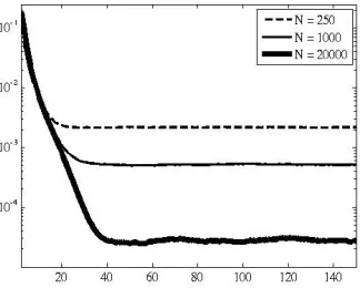
BothfaBS

N andfNaBS can be accurately numerically computed. Figure 1 shows simulation estimates off_NaBS(k)for small values ofkand different values ofN.

Figure 2 shows a representative example offBS

N (k)with a simulation estimate forN = 250.

FIG. 2. Plot offBS

250(k),k∈ {2, . . . ,50}.

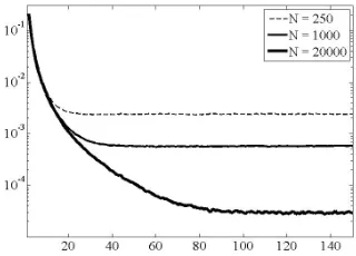
From the joint distribution we can compute the (indistinguishable) marginal distribution of ranks of the left and right neighbours,gBS

N (k). Representative examples are given in Figure 3.

FIG. 3. Plot ofgBS_N (k),k∈ {2, . . . ,150}forN = 250,1000,20000.

B. Thresholds

From the results of Figures 1–3 we see that for a givenN, the empirical distributions decay rapidly for smallkbefore settling down to a uniform value. In fact, it appears that there are constantsC1

andC2 such thatfNaBS(k) ≈ C1/N andgBSN (k) ≈ C2/N for large enoughk. Thus the numerical

C. Avalanches

Following [1] we define the length of ans-avalanche to betif the number of consecutive steps for which the smallest fitness value stays below s is t. Ass approaches s∗ we expectn(`), the dis-tribution ofs-avalanche lengths, to show the power law behaviour characteristic of self-organized criticality. UsingfaBS

N (k)andfNBS(k), we can compare the avalanches of RDPs with those of aBS and BS.

Consider the RDP induced by f_NaBS(k) (a similar approach can be adopted for BS, too). An s -avalanche of lengthlrepresents the end point of an excursion during the RDP whose starting point was the last time all states had fitnesses greater thans. Each excursion is a Markov chain whose state space is the number of states with fitness values belowsandn(l)is the distribution of arrival times at the absorbing state (zero fitnesses belows). The transition probabilities of the Markov chain can easily be calculated fromf_NaBS(k). Letpk =Pk_r=2fNaBS(r)andqk = 1−pk. Ifπkt is the probability that there arekstates less thansaftertsteps of the excursion then fork > 1,

π_tk₊₁ =s2qk−1πtk−1+ (s

2

pk+ 2s(1−s)qk)πkt +

(2s(1−s)pk+1+ (1−s)2qk+1)πkt+1+ (1−s)

2

pk+2πtk+2. (6)

Fork = 1we omit the first term on the right-hand side of (6) and

π_t0₊₁ =π_t0+ (1−s)2π_t1+ (1−s)2p2πt2.

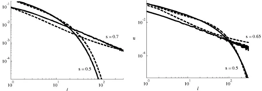
We compute the distributionn(l)ofs-avalanche lengths for various values ofsfor our RDPs and compare them with empirical results for aBS and BS. Representative distributions are given in Figure 4. There is a small but clear difference in the exponents of the two processes, but the RDP shows the characteristic behaviour expected assapproachess∗.

V. REMARKS

FIG. 4. Size distributionn(l)ofsavalanches in RDP (dashed) and aBS (left); and BS (right) forN = 2000.

to BS itself. The exact relationship of the two processes remains to be characterized rigorously. If one wished to define a Markov process on∆N whose stationary distribution coincided with the projection onto∆N of the stationary distribution of BS, a natural candidate would be a RDP with state-dependent selection distribution: instead of a singlefN(·)one would have a familyfN(·;x) of selection distributions conditioned on the statex ∈ ∆N. Thus, assuming it exists, one would takefN(·;x)to be fNBS(·;x), the stationary distribution for BS of the nearest neighbours of the smallest elementconditionalon the projection of the current state onto∆N beingx. The fact that the numerical evidence described above suggests that one can proceed not with a state-dependent RDP based on fBS

N (·;x)but with the simpler RDP based on fNBS(·)(which is an average of the

fBS

N (·;x)) seems to point to some important underlying property of BS itself. Two possible expla-nations are:

(a) fBS

N (·) = fNBS(·;x)for all x, i.e., at stationarity there is some independence between the order statistics and the permutation that maps sites to ranks; or

(b) fBS

N (·;x)satisfies (uniformly inx) the same asymptotic conditions asfNBS(·)that are central to the limit behaviour, namely (3) and (5).

processes share the same threshold and characteristic U[s∗,1]limit distribution. We remark that the distributionsfBS

N (·;x)seem to be very difficult to evaluate numerically. In conclusion, we have indicated how the distributionfBS

N (k, l)and the quantityα of (3) capture the build-up of correlations in Bak–Sneppen type algorithms, the threshold behaviour of which can be analysed exactly by considering the appropriate RDP.

The class of RDPs that we have introduced is of interest in its own right. The remaining analytical challenge is to clarify the relationship between BS and the RDP. This involves at least two main parts: (i) proving the existence of the distributionsf_NBS given by (1) and of the limitαdefined by (3); and (ii) determining the property of BS that allows us to usefBS

N (·)instead of the conditional version f_NBS(·;x). In respect to challenge (i) above, it is interesting to note that if an explicit description of fBS

N could be obtained, one might be able to obtain an explicit formula for the thresholds∗ via (3) and (4).

Appendix A: Derivation of the threshold formula

Consider thes-counting processC_tN(s)defined to be the number ofxk-values in the interval[0, s] aftertiterations of the RDP defined byfN. ThenCtN(s)is a Markov chain on the finite state-space

{0,1, . . . , N}. The thresholds∗relates to the limiting (t → ∞thenN → ∞) marginal distribution of an arbitrary xk. To evaluate s∗, we compute the mean drift of CtN(s), E[CtN+1(s)−CtN(s) |

CN

t (s) = n], whereE is the expectation operator. It can be shown that

E[C_tN₊₁(s)−C_tN(s)|C_tN(s) = n] =K(s−GN(n)).

Hence the drift is zero (asymptotically, asn→ ∞andN → ∞) at

s=s∗ = lim

n→∞Nlim→∞GN(n).

In terms of the functionsfN(i),FN(n)and the quantityα(3), we have that

gN(i) =

K −1

K fN(i)andGN(n) =

1 + (K−1)FN(n)

so that

s∗ = lim

n→∞Nlim→∞GN(n) =

1 + (K−1)α

K .

The drift being zero indicates the threshold behaviour, because a positive (negative) drift would meanC_tN(s) increases (decreases). In this argument there are several limits involved (n, N, tall going to∞) that need to be handled with care. In [2] we exploit techniques from Markov process theory, such as Foster–Lyapunov ideas [20], to do this.

ACKNOWLEDGMENTS

MG would like to acknowledge fruitful discussions with Gregory Berkolaiko, Jack Carr, Oliver Penrose, and Michael Wilkinson.

[1] P. Bak and K. Sneppen, Phys. Rev. Lett.,71, 4083 (1993).

[2] M. Grinfeld, P. A. Knight, and A. R. Wade, “Rank-driven Markov processes,” (2011), arXiv:1106.4194.

[3] H. Guiol, F. P. Machado, and R. B. Schinazi, “Diffuse X-ray emissions from dynamic planetary nebulae,” (2009), arXiv:1006.2595v1.

[4] A. K. Gupta, “Punctuated equilibrium and power law in economic dynamics,” (2010), arXiv:1012.5896v1.

[5] M. Bartolozzi, D. B. Leinweber, and A. W. Thomas, Physica A,365, 499 (2006). [6] M. Ausloos, P. Clippe, and A. Pe¸kalski, Physica A,332, 394 (2004).

[7] M. L. Lyra and U. Tirnakli, Physica D,193, 327 (2004). [8] J. Machta and X.-N. Li, Physica A,300, 245 (2001).

[9] J. Barbay and C. Kenyon, inProc. 12th Annual ACM-SIAM Symp. Discrete Algorithms(Washington, DC, 2001).

[10] D. A. Head and G. J. Rogers, J. Phys. A,31, 3977 (1998).

[12] G. J. M. Garcia and R. Dickman, Physica A,342, 516 (2004).

[13] H. Flyvbjerg, K. Sneppen, and P. Bak, Phys. Rev. Lett.,71, 4087 (1993).

[14] J. de Boer, B. Derrida, H. Flyvbjerg, A. D. Jackson, and T. Wettig, Phys. Rev. Lett.,73, 906 (1994). [15] G. L. Labzowsky and Y. M. Pis’mak, Phys. Lett. A,246, 377 (1998).

[16] C. Bandt, J. Stat. Phys.,120, 685 (2005).

[17] R. Meester and D. Znamenski, Ann. Probab.,31, 1986 (2003).

[18] A. Gillett, R. Meester, and D. Znamenski, J. Appl. Probab.,43, 840 (2006).

[19] A. J. Gillett, Phase transitions in Bak-Sneppen avalanches and in a continuum percolation model, Ph.D. thesis, Vrije Universiteit, Amsterdam (2007).