Demonstration of the temporal matter-wave Talbot effect for trapped matter waves

T h e o p e n – a c c e s s j o u r n a l f o r p h y s i c s

New Journal of Physics

Demonstration of the temporal matter-wave Talbot

effect for trapped matter waves

Manfred J Mark1, Elmar Haller1, Johann G Danzl1, Katharina Lauber1, Mattias Gustavsson2 and Hanns-Christoph Nägerl1,3

1_{Institut für Experimentalphysik und Zentrum für Quantenphysik,}

Universität Innsbruck, Technikerstraße 25, A-6020 Innsbruck, Austria 2_{Department of Physics, Yale University, PO Box 208120, New Haven,}

CT 06520, USA

E-mail:[email protected]

New Journal of Physics13(2011) 085008 (15pp) Received 30 April 2011

Published 10 August 2011 Online athttp://www.njp.org/ doi:10.1088/1367-2630/13/8/085008

Abstract. We demonstrate the temporal Talbot effect for trapped matter waves using ultracold atoms in an optical lattice. We investigate the phase evolution of an array of essentially non-interacting matter waves and observe matter-wave collapse and revival in the form of a Talbot interference pattern. By using long expansion times, we image momentum space with sub-recoil resolution, allowing us to observe fractional Talbot fringes up to tenth order.

Contents

1. Introduction 2

2. Preparation of the initial sample 3

3. Phase evolution and the Talbot effect 4

4. Experimental realization 6

5. Conclusion 11

Acknowledgments 14

References 14

3_{Author to whom any correspondence should be addressed.}

1. Introduction

Interference of matter waves is one of the basic ingredients of modern quantum physics. It has proved to be a very rich phenomenon and has found many applications in fundamental physics as well as in metrology [1] since the first electron diffraction experiments by Davisson and Germer [2]. Matter-wave optics has now developed into a thriving subfield of quantum physics. Many key experiments from classical optics have found their counterpart with matter waves, for example the realization of Young’s double-slit experiment with electrons [3], the implementation of a Mach–Zehnder-type interferometer with neutrons [4] or, more recently, the observation of Poisson’s spot with molecules [5]. The creation of Bose–Einstein con-densates (BECs) in 1995 [6, 7] opened the door to many more exciting experiments with matter waves, to a large extent in the same way as the laser did in the case of classical light waves.

One remarkable phenomenon in classical optics is the Talbot effect, the self-imaging of a periodic structure in near-field diffraction [8]. The effect was first observed by Talbot in 1836 [9] and was later explained in the context of wave optics by Rayleigh in 1881 [10]. When light with a wavelengthλilluminates a material grating with periodd, the intensity pattern of light passing through the grating reproduces the structure of the grating at distances behind the grating equal to odd multiples of the so-called Talbot lengthL_Talbot=d2/λ_{. At even multiples of Talbot length,} the intensity pattern again reproduces the structure of the grating, but shifted laterally in space by half the grating period. In between these recurrences, at rational fractions n/m of L_Talbot

(withn,m coprime), patterns with smaller periodd/m are formed. This effect is known as the fractional Talbot effect. A necessary requirement for the appearance of the Talbot effect and its fractional variation is the validity of the paraxial approximation [11]. Crucial to the Talbot effect is the fact that the accumulated phase differences of propagating waves behind the grating show a quadratic dependence on lateral distance or grating slit index.

mean-field interaction, which had a quadratic spatial dependence reflecting the parabolic shape of the initial density distribution.

In this paper, we report on the demonstration of the temporal Talbot effect using trapped, non-interacting matter waves. Here, the Talbot effect is not driven by interactions but by the (weak) external harmonic dipole trap confinement, leading to a characteristic quadratic phase evolution. Unlike our earlier work [20], the contrast of the Talbot pattern is not degraded by interaction-driven on-site phase diffusion [21], allowing us to follow the phase evolution for long times and hence allowing us to observe matter-wave revivals. For our measurements, we use as before an array of pancake-shaped, 2D BECs in a 1D optical lattice [20]. The optical lattice takes on the role of the grating. Cancelling the effect of interactions in the vicinity of a Feshbach resonance and decoupling the individual BECs by means of a gravitational tilt initiate long-lived Bloch oscillations (BOs) in momentum space [22]. These are quickly superimposed by a Talbot-type interference pattern in the presence of external confinement. The pattern can be directly connected to the (fractional) Talbot effect. In particular, after specific hold times that are multiples of the Talbot time, the time analogue to the Talbot length, a rephasing of the momentum distribution can be observed.

2. Preparation of the initial sample

We first produce an essentially pure BEC of Cs atoms (no detectable non-condensed fraction) by largely following the procedure detailed in [23, 24]. The atoms are in the lowest hyperfine sublevel F ₌3, mF =3 trapped in a crossed optical dipole trap and initially levitated against gravity by a magnetic gradient field. As usual, F is the atomic angular momentum quantum number, and mF is its projection on the magnetic field axis. For the present experiments, the atom number is set typically to 6×104 _{atoms. The trap frequencies in the crossed dipole trap} are chosen to beωx =2π×21.7(3)Hz,ωy=2π×26.7(3)Hz andωz=2π×26.9(3)Hz. The confinement along the vertical axis (z) and the two horizontal axes (x,y) is controlled by two horizontally propagating dipole trap beams with beam waists of 46 and 144µm and one vertically propagating dipole trap beam with a beam waist of 123µm. The atomic scattering length as and therefore the strength of interactions in the BEC can be tuned via a magnetic offset field B in a range between as=0a0 and as=1000a0 by setting B to values between approximately 17 and 46 G using a magnetically induced Feshbach resonance [25], as illustrated in figure 1(a). Here, a0 is Bohr’s radius. For the initial preparation of the sample, we setas to positive values, typically between 100a0and 210a0. Later,asis set to zero as discussed below. We gently load the condensed atomic sample into a vertical standing wave, as illustrated in figure 1(b), by exponentially ramping up the power in the standing wave over the course of about 1000 ms. The standing wave is generated by a retro-reflected laser beam at a wavelength of λ=1064.48(5)nm with a 1/e waist of about 350µm. We are able to achieve well depths of up to 40E_R, where E_{R= ¯}h2k2/(_2m)_=h2/(_2mλ2)_=k

0.0 0.1 0.2 0.3 0.4 0.5 0.6 0.7 0.8 0.9 1.0 −1

−0.5 0 0.5 1

Momentum (ħk)

Hold time thold (TBloch)

10 20 30 40 50 60

-1.5 -1 -0.5 0 0.5 1 1.5

Scattering length a

S

(x10

3 a

0

)

Magnetic field B (G)

(a)

(b)

(c)

x y z

Figure 1. (a) Magnetic field dependence of the scattering length a_s for Cs atoms in F₌3,mF =3: wide tunability is given by a broad magnetic Feshbach resonance with a pole near−11 G (not shown), leading to a region with attractive interaction, a zero crossing at about 17 G and a repulsive region above [25]. Two narrow Feshbach resonances can be seen in the vicinity of 50 G. (b) Experimental configuration: a vertically oriented standing laser wave creating a stack of pancake-shaped traps is intersected by two horizontal laser beams. (c) BOs: time series in steps of about 57µs showing the quasi-momentum distribution over the course of one Bloch cycle.

3. Phase evolution and the Talbot effect

Our system, the BEC loaded into a 1D optical lattice with spacingd₌λ/2, can be modelled by a discrete nonlinear equation (DNLE) in one dimension [27], as discussed in our earlier work [20]. In brief, this equation can be obtained by expanding the condensate wave function from the Gross–Pitaevskii equation, 9, in a basis of wave functions 9j(z,r⊥) centred at individual

lattice sites with index j,9(z,r_⊥,t)₌P

jcj(t)9j(z,r⊥). Here, z is the coordinate along the

amplitudes. The atoms are restricted to moving in the lowest Bloch band and we can write

9j(r⊥,z)=w(

j)

0 (z)8⊥(ρj,r⊥), wherew(

j)

0 (z)are the lowest-band Wannier functions localized at the jth site and8⊥(ρj,r⊥)is a radial wave function depending on the peak densityρj at each site [27]. By inserting this form into the Gross–Pitaevskii equation and integrating out the radial direction, the DNLE is obtained,

ih_¯∂cj

∂t = J(cj−1+cj+1)+E

int

j (cj)cj+Vjcj. (1)

Here, J/his the tunnelling rate between neighbouring lattice sites,Vj =Fd j+V trap

j describes the combination of a linear potential with force F and an external, possibly time-varying trapping potentialV_jtrap, and Eint_j (cj)is the nonlinear term due to interactions.

We first load the BEC into the vertical lattice and then allow the gravitational force to tilt the lattice potential. We thus enter the limit FdJ, in which tunnelling between sites is inhibited and the on-site occupation numbers|cj|2are constant, determined by the initial density distribution. The time evolution of the system is then given by the time-dependent phases of all

cj, and the 1D wave function9(˜ q,t)in quasi-momentum spaceqacquires a particularly simple form [28]:

˜

9(q,t)₌ X

j

cj(t)e−iq j d =

X

j

cj(0)e−i(Fd j+ V_jtrap+Eint

j )t/¯h_e−iq j d

= X

j

cj(0)e−i(q+ Ft

¯

h )j de−i(βtr(j−δ)2−αint(j−δ)2)t/¯h. ₍₂₎

Here, we have assumed that our external potential is harmonic, given by V_jtrap₌β_tr(j₋δ)2_, where βtr=mω2zd2/2 characterizes the strength of the potential with trapping frequency ωz along z for a particle with mass m. The parameter δ in the interval [−1/2,1/2] describes a possible offset of the potential centre with respect to the nearest lattice well minimum along the

z-direction. For the interaction termαint, the spatial dependence is also parabolic, reflecting the fact that we initially load a (parabolically shaped) BEC in the Thomas–Fermi regime. In our experiments, the offsetδis not well controlled. It is nearly constant on the timescale of a single experimental run (duration of up to 20 s), but its value changes over the course of minutes as the positions of the horizontally propagating laser beams generating the trapping potential and the position of the retro-reflecting mirror generating the vertical standing wave drift due to changes of the ambient conditions.

it is irrelevant for the Talbot effect, we setδ to zero here. By including the simplifications and introducing the Talbot time T_Talbot=h/(mω2

zd2), equation (2) reduces to

˜

9(q,t)₌X

j

cj(0,q)e−iπj 2_t/(2T

Talbot) ₍₃₎

with cj(0,q)=cj(0)exp(−i q j d). Now the Talbot effect is evident. For times that are even

multiples of T_Talbot the original wave function is recovered, whereas for odd multiples the original wave function appears with a shift of _¯hk in quasi-momentum space. This realization of the Talbot effect is nearly ideal, since no paraxial approximation is needed and since there is no limitation in time due to decreasing wave packet overlap [19]. For fractions n/m of T_Talbot,

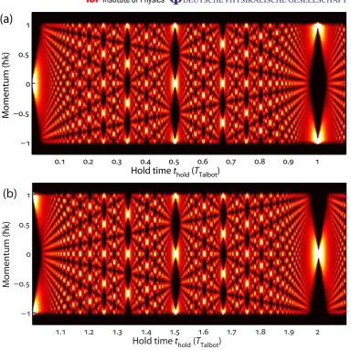
m copies of the original wave function with a spacing 2hk_¯ /m appear, corresponding to the fractional Talbot effect. The evolution of the quasi-momentum distribution as a function of time can be visualized in terms of so-called matter-wave quantum carpets [31, 32]. Such a quantum carpet, calculated by solving equation (1) numerically with parameters typical to our experiment, is shown in figure 2. Note that in this case the more simple calculation based on equation (3) leads to the same result. However, equation (1) gives us more flexibility in relaxing the requirements of harmonic confinement or negligible tunnelling. We plot the distribution as a line density plot, with white areas indicating high densities. Only times that are integer multiples ofT_Blochare shown. After a fast spreading of the quasi-momentum distribution, a regular pattern appears at times for which one expects fractional Talbot interferences. The number of peaks in the momentum distributions directly represents the fraction t/T_Talbot. At T_Talbot a refocusing to the initial distribution occurs, shifted by hk_¯ in quasi-momentum space. The evolution is then repeated until at 2T_Talbot the original wave function is recovered.

4. Experimental realization

For the present experiments, we choose a lattice depth of 8ER. For lattice loading, the interaction strength is set to as=100a0 and the external trap frequencies are changed adiabatically to populate about 40 lattice sites. After loading, we change ωz to the final value. This change is done sufficiently quickly (within 3 ms) to avoid a change in the initial distribution due to tunnelling, but sufficiently slowly to avoid motional excitations along the z-direction. Then, within 0.1 ms, we switch off the levitating magnetic field gradient to decouple the individual lattice sites and set the scattering length to the value near a_s=0a₀ that gives minimal dephasing [22]. Note that the point of minimal dephasing does not correspond exactly to 0a₀

Momentum (ħk)

Hold time t_hold (T_Talbot)

1.1 1.2 1.3 1.4 1.5 1.6 1.7 1.8 1.9 2

−1 −0.5 0 0.5 1

Momentum (

ħk

)

Hold time t_hold (T_Talbot)

0.1 0.2 0.3 0.4 0.5 0.6 0.7 0.8 0.9 1

−1 −0.5 0 0.5 1

(a)

(b)

Figure 2. Calculated BEC-based temporal Talbot effect. (a) Momentum distribution as a function of hold time thold starting from the initial BEC to the first revival at TTalbot for a pure harmonic potential. White areas indicate a high occupation of the respective momentum state. (b) Same as in (a) from

t_hold=T_Talbottot_hold=2T_Talbot.

the momentum width1pas two times the second moment of the momentum distribution along the vertical direction. Note that the presence of the horizontal trap during expansion leads to additional broadening in the vertical direction. This broadening plus some residual incoherent background limits the observable values of 1p. Nevertheless, with our ability to image the quasi-momentum with high resolution [20], we are able to compare not only the momentum width but also the substructure in the momentum distribution to theory.

-1 -0.5 0 0.5 1

M

omentum (ħk)

Hold time thold (TTalbot)

0 1/10 1/9 1/8 1/7 1/6 1/5 1/4 1/3 1/2 1

−1 −0.5 0 0.5 1

Momentum (ħk)

Hold time thold (TTalbot)

(a)

(b)

0 1/10 1/9 1/8 1/7 1/6 1/5 1/4 1/3 1/2 1

Figure 3. BEC-based temporal Talbot effect—experiment. (a) Series of absorption images after 80 ms of expansion, showing fractional Talbot fringes of different order in momentum space, starting from the initial momentum distribution of the BEC after two BOs (left), followed by the tenth order at

T_Talbot/10, ninth order atT_Talbot/9, etc, down to the zeroth order at the Talbot time (right). Note that the time axis is not linear. White areas indicate higher density. (b) Horizontally integrated density profiles obtained from the absorption images shown in (a). Note that, for example, for T_Talbot/10, the outermost momentum component appears twice, i.e. at both edges of the Brillouin zone.

non-dephased BEC. After a rapid coherent dephasing (corresponding to a rapid broadening of the momentum distribution, not shown here), regularly structured patterns appear. The number of peaks within the first Brillouin zone [_−¯hk,+_¯hk] corresponds exactly to the fraction

0 1 2 3 4 -1

-0.5 0 0.5 1

M

omentum (ħk)

Experimental run

0 1 2 3 4

-1 -0.5 0 0.5 1

M

omentum (ħk)

Experimental run

0 1 2 3 4

−1 −0.5 0 0.5 1

Momentum (ħk)

Experimental run

(a)

(b)

(d)

0 1 2 3 4

−1 −0.5 0 0.5 1

Momentum (ħk)

Experimental run

(c)

Figure 4. Variations in the momentum distribution between successive experimental realizations for long hold times. (a) Absorption images of five individual experimental realizations with thold=TTalbot. White areas indicate higher density. (b) Horizontally integrated density profiles obtained from the absorption images shown in (a). (c) Absorption images of five individual experimental realizations with t_hold=T_Talbot/2. (d) Horizontally integrated density profiles obtained from the absorption images shown in (c). Note that, in addition to the random shift in quasi-momentum space caused byδ, effects of horizontal dynamics, especially fragmentation and density variations along the horizontal axis, can be observed.

is calculated to be_±¯hk_×t_hold/T_Talbot. This is why the patterns shown in figure3, for example, at t_hold=T_Talbot or at t_hold=T_Talbot/2, agree with the calculated patterns only modulo the shift in quasi-momentum space. Note that, alternatively, we could have chosen to present in figure3

selected patterns from a sufficiently large sample of measurements, for example, the one from experimental run 4 for thold=TTalbot or the one from experimental run 1 for thold=TTalbot/2 shown in figure4.

A simple quantitative comparison between experiment and calculations can be done by considering the time evolution of the momentum width 1p. The distribution of this quantity across several experimental realizations is evidently sensitive to the de- and rephasing of the matter wave. In fact, we can relax the choice of the Bloch phase and allow its value to be random. For example, for a non-dephased BEC the momentum width 1p is measured to range from (1p)_min≈0.6_¯hk, corresponding to the singly peaked momentum distribution, to

(1p)_max≈1.7hk_¯ , when the momentum distribution is evenly peaked at both edges of the Brillouin zone (e.g. at half the first Bloch period; see figure 1(c)). For a completely dephased sample corresponding to a uniform distribution over the first Brillouin zone, we measure a value of1p_≈1.25hk_¯ . Accordingly, the range for the momentum width1pat a given hold timet_hold

shows distinct behaviour as a function of t_hold, in particular indicating the revival at T_Talbot by maximizing the difference D₁p=(1p)max−(1p)min between the extrema of1p. Figure5(a) shows (1p)maxand(1p)min as a function ofthold as calculated from equation (1). Initially and at TTalbot the extrema lie far apart (at these times the calculation gives values for(1p)min that are close to zero in accordance with the fact that the momentum width is determined only by the spread in position space, which is large), whereas at intermediate times the difference is drastically reduced, only increasing slightly at rational fractions of thold/TTalbot. In figure5(b), we plot the measured momentum width extrema. These are determined from samples of ten single measurements at each chosen value for t_hold. The initial rapid collapse agrees well with the fact that the sample dephases. Then, near the calculated value forT_Talbot, a clear increase in

D_1p can be seen. The difference recovers almost completely to the initial value. We attribute the slight reduction to additional dephasing mechanisms not included in our simple model, as discussed below.

The behaviour of D_1p offers a simple method to test the dependence of the Talbot time

TTalbot on the vertical trap frequencyωz. Evidently, D1p has a maximum at TTalbot. Figure6(a) shows the momentum width 1p in the vicinity of the calculated TTalbot, here for a specific trap frequency of ωz=2π×26.9(2)Hz. Again we evaluate ten experimental realizations for each hold time and select(1p)max and(1p)minto calculate D1p. We locate the position of its maximum by a simple Gaussian fit, as shown in figure 6(b). We then vary ωz and determine

T_Talbot accordingly. In figure 6(c), T_Talbot is plotted as a function of ωz. The experimental values are in excellent agreement with the calculated values for the Talbot time according to

T_Talbot=h/(mω2 zd2).

0.1 0.2 0.3 0.4 0.5 0.6 0.7 0.8 0.9 1 0

0.5 1 1.5 2

M

omentum width ∆

p

(ħk)

Hold time tHold (TTalbot)

0.1 0.2 0.3 0.4 0.5 0.6 0.7 0.8 0.9 1

0.5 1 1.5 2

M

o

mentum width Δ

p

(ħk)

Hold time thold (TTalbot)

(a)

(b)

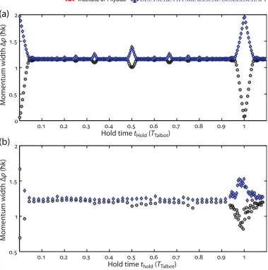
Figure 5. Talbot revival as evidenced by the spread of momentum width 1p. (a) Calculated(1p)max(blue diamonds) and(1p)min(black circles) as a function of thold in units of TTalbot. (b) Measurement of (1p)max (blue diamonds) and

(1p)_min(black circles) as a function of t_hold in units of T_Talbot for a vertical trap frequency ofωz=2π×22.0(2)Hz. The extrema are determined from a sample of ten single experimental realizations for each value oft_hold.

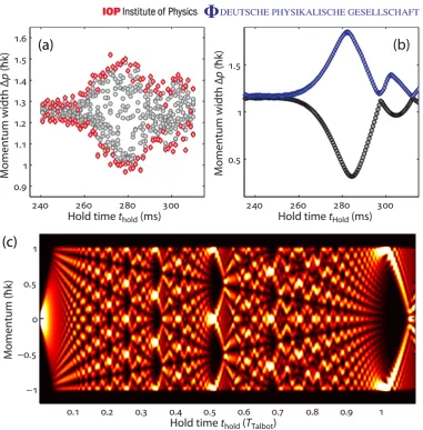
non-perfect Talbot revivals followed by subrevivals as can be seen in figure 7(a). This is in qualitative agreement with calculations shown in figure7(b), for which the real Gaussian shape of the trapping potential instead of a simple harmonic one has been used. The full calculated time evolution of the momentum distribution is shown in figure 7(c). The distortion of the matter-wave quantum carpet can clearly be seen.

5. Conclusion

20 25 30 35 40 45 50 100

200 300 400 500 600

Talbot time

TTalbot

(ms)

Trap frequency νz (Hz)

340 360 380

0.9 1 1.1 1.2 1.3 1.4 1.5 1.6

p

(ħk)

Hold time thold (ms)

340 360 380

0 0.1 0.2 0.3 0.4 0.5 0.6

∆p

(ħk)

Hold time thold (ms)

(a)

(b)

(c)

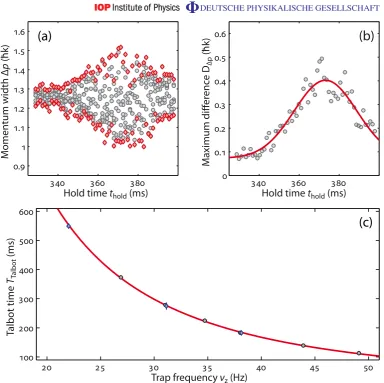
Figure 6. Talbot time T_Talbot as a function of external confinement strength. (a) Momentum width 1p in the vicinity of the expected T_Talbot for a dipole trap frequency ofωz=2π×26.9(2)Hz for ten single experimental realizations (black circles). The extrema(1p)_maxand(1p)_minare indicated as red diamonds. (b) Calculated D₁p for the measured extrema in (a). The solid line represents a Gaussian fit, from which TTalbot is derived. (c) Dependence of TTalbot on trap frequency νz=ωz/(2π). The black (blue) circles (diamonds) represent measurements for which the external harmonic trap is generated by the dipole trap beam with a 46µm (144µm) beam waist. The solid line gives the calculated values forT_Talbot. The vertical error bars are the 1σ uncertainty of the maximum position of the Gaussian fit as shown in (b). The horizontal error bars are equal to or smaller than symbol size.

240 260 280 300 0.5

1 1.5

M

omentum width ∆

p

(ħk)

Hold time tHold (ms)

Momentum (ħk)

Hold time thold (TTalbot)

0.1 0.2 0.3 0.4 0.5 0.6 0.7 0.8 0.9 1

−1 −0.5 0 0.5 1

240 260 280 300

0.9 1 1.1 1.2 1.3 1.4 1.5 1.6

M

omentum width Δ

p

(ħk)

Hold time thold (ms)

(a)

(b)

(c)

Figure 7.The effect of anharmonic trapping potential on momentum distribution. (a) Momentum width1pin the vicinity of the expectedTTalbot for a dipole trap frequency of 2π_×31.1(2)Hz for ten single experimental realizations (black circles). The vertical dipole trap is created by the more tightly focused dipole trap beam with a beam waist of 46µm. The extrema (1p)_max and (1p)_min are indicated as red diamonds. (b) Calculated (1p)_max and (1p)_min in the vicinity of the expected T_Talbot for the same experimental parameters as in (a). For the trapping potential, the real Gaussian shape of the dipole trap is used. (c) Full calculation of the momentum distribution as a function of hold timet_hold using the same parameters as in (b).

Acknowledgments

We are indebted to R Grimm for generous support and we thank A Daley for valuable discussions. We gratefully acknowledge funding by the Austrian Science Fund (FWF) within project I153-N16 and within the framework of the European Science Foundation (ESF) EuroQUASAR collective research project QuDeGPM.

References

[1] Cronin A D, Schmiedmayer J and Pritchard D E 2009Rev. Mod. Phys.811051–129 [2] Davisson C and Germer L H 1927Phys. Rev.30705–40

[3] Jönsson C 1961Z. Phys.161454–74

[4] Rauch H, Treimer W and Bonse U 1974Phys. Lett.A47369–71

[5] Reisinger T, Patel A A, Reingruber H, Fladischer K, Ernst W E, Bracco G, Smith H I and Holst B 2009Phys. Rev.A79053823

[6] Anderson M H, Ensher J R, Matthews M R, Wieman C E and Cornell E A 1995Science269198

[7] Davis K B, Mewes M O, Andrews M R, van Druten N J, Durfee D S, Kurn D M and Ketterle W 1995Phys.

Rev. Lett.753969–73

[8] Berry M, Marzoli I and Schleich W P 2001Phys. World1439–44 [9] Talbot H F 1836Phil. Magn.9401

[10] Rayleigh L 1881Phil. Magn.11196–205 [11] Patorski K 1989Prog. Opt.271–108

[12] Schmiedmayer J, Ekstrom C R, Chapman M S, Hammond T D and Pritchard D E 1993 Fundamentals

of Quantum Optics III Proc. Kühtai Austriaed F Ehlotzky (Lecture Notes in Physicsvol 420) (Berlin:

Springer)

[13] Chapman M S, Ekstrom C R, Hammond T D, Schmiedmayer J, Tannian B E, Wehinger S and Pritchard D E

1995Phys. Rev.A51R14–7

[14] Nowak S, Kurtsiefer Ch, Pfau T and David C 1997Opt. Lett.221430–2 [15] Lau E 1948Ann. Phys.6417

[16] Clauser J F and Li S 1994Phys. Rev.A49R2213–6

[17] Brezger B, Hackermüller L, Uttenthaler S, Petschinka J, Arndt M and Zeilinger A 2002 Phys. Rev. Lett. 88100404

[18] Gerlich Set al2007Nature Phys.3711–5

[19] Deng L, Hagley E W, Denschlag J, Simsarian J E, Edwards M, Clark C W, Helmerson K, Rolston S L and Phillips W D 1999Phys. Rev. Lett.835407–11

[20] Gustavsson M, Haller E, Mark M J, Danzl J G, Hart R, Daley A J and Nägerl H-C 2010 New J. Phys. 12065029

[21] Li W, Tuchman A K, Chien H-C and Kasevich M A 2007Phys. Rev. Lett.98040402

[22] Gustavsson M, Haller E, Mark M J, Danzl J G, Rojas-Kopeinig G and Nägerl H-C 2008 Phys. Rev. Lett. 100080404

[23] Weber T, Herbig J, Mark M, Nägerl H-C and Grimm R 2003Science299232

[24] Kraemer T, Herbig J, Mark M, Weber T, Chin C, Nägerl H C and Grimm R 2004Appl. Phys.B791013–9 [25] Chin C, Vuleti´c V, Kerman A J, Chu S, Tiesinga E, Leo P J and Williams C J 2004Phys. Rev.A70032701 [26] Liem A, Limpert J, Zellmer H and Tünnermann A 2003Opt. Lett.281537–9

[27] Smerzi A and Trombettoni A 2003Phys. Rev.A68023613

[28] Witthaut D, Werder M, Mossmann S and Korsch H J 2005Phys. Rev.E71036625

[29] Ben Dahan M, Peik E, Reichel J, Castin Y and Salomon C 1996Phys. Rev. Lett.764508–11 [30] Anderson B P and Kasevich M A 1998Science2821686

[32] Ruostekoski J, Kneer B, Schleich W P and Rempe G 2001Phys. Rev.A63043613

[33] Fattori M, Roati G, Deissler B, D’Errico C, Zaccanti M, Jona-Lasinio M, Santos L, Inguscio M and Modugno G 2008Phys. Rev. Lett.101190405

[34] Kastberg A, Phillips W D, Rolston S L, Spreeuw R J C and Jessen P S 2008Phys. Rev. Lett.741542–5 [35] Casimir H B G and Polder D 1948Phys. Rev.73360