Modelling the effect of recent stress history on the deformation of overconsolidated soils

City, University of London Institutional Repository

Citation:

This is the accepted version of the paper.

This version of the publication may differ from the final published

version.

Permanent repository link:

Link to published version:

Copyright and reuse: City Research Online aims to make research

outputs of City, University of London available to a wider audience.

Copyright and Moral Rights remain with the author(s) and/or copyright

holders. URLs from City Research Online may be freely distributed and

linked to.

City Research Online: http://openaccess.city.ac.uk/ publications@city.ac.uk

MODELLING THE EFFECT OF RECENT STRESS HISTORY ON THE DEFORMATION OF OVERCONSOLIDATED SOILS

by

Sarah Elizabeth Stallebrass

A Thesis submitted for the Degree of Doctor of Philosphy

THE CITY UNIVERSITY Civil Engineering Department

CONTENTS

List of Tables 6

List of Figures 7

Acknowledgements 18

Declaration 19

List of Symbols 20

CHAPTER 1 INTRODUCTION 25

1.1 Background to the project 25

1.2 Basic framework 26

1.2.1 Basic methodology of the research 26

1.2.2 Theoretical framework 28

1.2.3 Interpretation of data 30

CHAPTER 2 LITERATURE REVIEW 33

2.1 Introduction 33

2.2 Development of experimental techniques in 34

laboratory testing

2.2.1 Developments in hydraulic stress path 34

cells

2.2.2 Developments in strain measuring 35

techniques

2.3 Experimental investigation of deformations 39

at small strains

2.4 Soil models for the stress-strain behaviour 44

of overconsolidated soil

2.4.1 Elastic models 44

2.4.2 Yielding models 48

2.5 Summary 51

CHAPTER 3 EXPERIMENTAL WORX 52

3.1 Introduction 52

3.2 Apparatus 53

3 . 2. 2 Instrumentation 54

3.2.3 Accuracy of measurements 55

3.3 Soil used in the experimental work 58

3.4 Sample preparation 59

3.4.1 Undisturbed samples 59

3.4.2 Reconstituted samples 60

3.5 Test procedure 61

3.5.1 Setting up the sample 61

3.5.2 Saturation stages 62

3.5.3 Initial compression stage 63

3.5.4 Main loading stages 64

3.5.5 Final stages 64

3.6 Test description 64

3.6.1 Objectives 64

3.6.2 Description of basic test 65

3.6.3 Test categories 67

CHAPTER 4 THE EFFECT OF RECENT STRESS HISTORY ON SOIL 69

BEHAVIOUR OBSERVED IN lABORATORY TESTS

4.1 Introduction 69

4.2 Experimental data obtained during current 71

research project

4.2.1 Quality of data 71

4.2.2 Analysis of results 76

4.2.3 Behaviour of undisturbed soil samples 78

4.2.4 Influence of state and overconsolidation 80 ratio

4.2.5 Strain increment ratios, undrained 85

effective stress paths

4.3 Evaluation of data from Richardson (1988) 88

4.3.1 Data as presented 88

4.3.2 Re-intepretation of data 93

4.4 Evaluation of data from 'True Triaxial' test 94

4.4.1 Introduction 94

4.4.2 Description of test 95

4.4.3 Results 96

4.5 Summary of experimental data 97

4.6 Implications for numerical modelling 100

4.6.1 Major characteristics to be modelled 100

CHAPTER 5 NUMERICAL MODELLING 102

5.1 Introduction 102

5.2 Evaluation of existing models 102

5.3 Two-surface "Bubble" model - Al Tabbaa (1987) 104 and Al Tabbaa and Wood (1989)

5.3.1 Description of model 104

5.3.2 Calculation of model parameters 109

5.3.3 Evaluation of model predictions 112

5.4 Three-surface yield model 115

5.4.1 Basic description of the model 115

5.4.2 Translation rules 116

5.4.3 Hardening rule 120

5.4.4 Calculation of model parameters 125

5.4.5 Validation of the computer program 127

TERTIUS

5.4.6 Parametric study 129

5.4.7 General characteristics of the three- 133

surface model

5.5 Evaluation of model 135

5.5 .1 Introduction 135

5.5.2 Non-linearity and inelasticity 136

5.5.3 Influence of recent stress history 137

5.5.4 Undrained compression tests 141

5.5.5 Different soils and time effects 141

5.5.6 Summary 142

CHAPTER 6 SUMNARY AND CONCLUSIONS 144

6.1 Effect of recent stress history on the 144

behaviour of overconsolidated soils

6.1.1 Typical characteristics 144

6.1.2 Effect of recent stress history on 145

undisturbed soil samples

6.1.3 Detailed features of recent stress 145

history effects

6.2 Modelling the recent stress history effect l4S

6.2.1 Why use a three-surface model 147

6.2.2 Model parameters 147

6.2.3 Evaluation of model predictions against 148 experimental data

6.3 Further work 150

6.3.1 Further experimental work 150

6.4 Conclusions 152

APPENDI CES 154

Appendix I - Flow chart for the computer program 154 S ECUNDUS

Appendix II - Flow chart for the computer program 155 TERTIUS

References 156

LIST OF TABLES

Table 3.2.1 Tables showing the accuracy of (a) stress and (b) strain transducers.

Table 3.3.1 (a) t 00 of soil used in stress path tests. (b) Typical critical state parameters for London Clay and speswhite kaolin.

Table 3.3.2 Location and estimated in situ state of undisturbed samples of London clay.

Table 3.6.1 Initial and final states of soil samples used in all stress path tests.

Table 3.6.2 (a) Description of tests on samples of undisturbed London clay. (b) Description of tests with an undrained common stress path using smples of reconstituted soil. (c) Description of drained, constant p' and constant q' tests on samples of reconstituted soil.

Tabel 4.2.1 Table showing the estimated overall history and the state at the start of the common path for the six tests on undisturbed London clay.

Table 4.3.1 Summary of tests conducted by Richardson (1988) to investigate the influence of recent stress history. (after Richardson, 1988)

Table 4.3.2 The effect of periods of rest on the stiffness of London clay. (after Richardson, 1988)

LIST OF FIGURES

Figure 1.2.1 Diagram defining the main parameters used in the Modified Cain-clay model.

Figure 1.2.2 Diagram showing a typical set of stress probes for the basic test to investigate the recent stress history effect.

Figure 1.2.3

Figure 1.2.4

Figure 2.2.1

Diagram showing the definition of p for (a) isotropic and (b) anisotropic loading.

Diagram defining p, the equivalent pressure in mv lnp' space

Cross-section of the hydraulic stress path cell. (after Bishop and Wesley, 1975)

Figure 2.2.2 General arrangement for the measurement of axial strains inside the cell using miniature LVDTs. (after Costa Filho, 1985)

Figure 2.2.3 Sketch showing the construction of the electrolevel strain gauges and the way in which axial strain is converted to rotation of the capsule. (after Jardine et al, 1984)

Figure 2.2.4

Figure 2.2.5

Figure 2.2.6

Sketch showing the design of pendulum inclinometer gauges. (after Ackerly et al, 1987)

Configuration of Hall effect axial and radial strain gauges. (after Clayton et al, 1989)

Sources of error in external measurements. (after Jardine et al, 1984)

Figure 2.3.1 Comparison between stress-strain curves for unconsolidated undrained tests and anisotropically consolidated undrained tests on samples of undisturbed London clay. (after Costa Filho, 1979)

Figure 2.3.2 Sketched boundaries for zones of different classes of deformation after K., consolidation, after perfect sampling and after extension to 5% axial strain tests on North Sea clay. (after Jardine, 1985)

Figure 2.3.3 Graph showing the decay of shear stiffness, C, normalised by the initial shear stiffness, C O3 with torsional shear strain for a selection of tests on Todi clay. (after Rampello, 1989)

Figure 2.3.5 Graphs showing the effect of recent stress history on the stress-strain response of London clay along constant p' extension and compression paths at p' -200kPa, p'm - 400kPa. (after Atkinson et al. 1990) Figure 2.4.1 Diagram showing the definition of the constants in the

periodic logarithmic function used to curve fit non-linear stiffness-strain data. (after Jardine et al, 1986)

Figure 2.4.2 Diagram describing the kinematic yield surface effect. (after Simpson et al, 1979)

Figure 2.4.3 Schematic illustration of the bounding surface and definition of image points in general stress space.

(after Dafalias and Herrman, 1982)

Figure 2.4.4 Relative configuration of the yield and consolidation surfaces in the two-surface model (a) after isotropic consolidation OA (b) for the stress history OAP 1 P2 -P3 . (after Mröz et al, 1979)

Figure 2.4.5 Model with an infinite number of surfaces: (a) first reverse loading (b) second reverse loading. (after MrOz and Norris, 1982)

Figure 2.4.6 Typical configuration of surfaces in the three-surface model proposed by Hashiguchi (1985). (after Hashiguchi, 1985) Figure 3.2.1 Figure 3.2.2 Figure 3.2.3 Figure 3.2.4 Figure 3.2.5 Figure 3.2.6 Figure 3.2.7

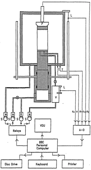
Schematic diagram of "Spectra" control system for stress path cells used to test 38mm diameter samples. Schematic diagram of "BBC" control system for stress path cells used to test 38mm diameter samples.

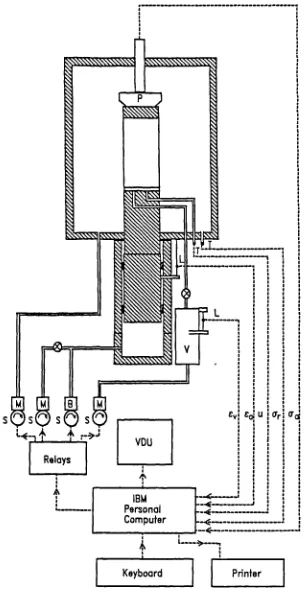
Schematic diagram of "IBM" control system for stress path cells used to test 100mm diameter samples.

Typical calibration curve for a LVDT used to measure axial strains.

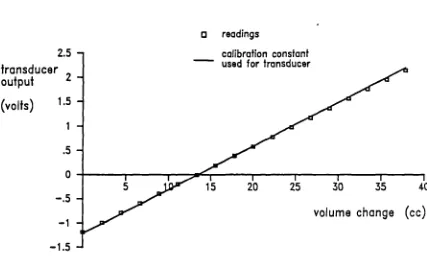
Typical calibration curve for a LVDT used with a volume gauge.

Typical calibration curve for a Hall effect local axial strain gauge.

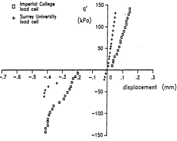
Compliance curves for Imperial College and Surrey University designed load cells.

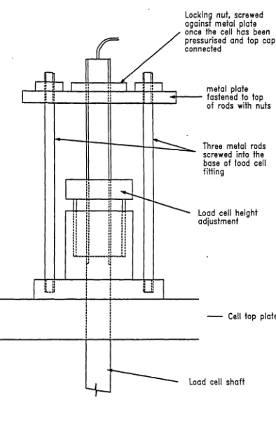
Figure 3.2.8 Diagram showing the simple restraining device used to stop movement of the load cell shaft. (after Cherrill, 1990)

Figure 3.3.1 (a) Typical soil profile (b) Typical porewater and K.,, profiles for Site 1 in north London.

Figure 3.4.1 Diagram of perspex floating ring consolidation press. Figure 3.5.1

Figure 3.5.2

Figure 3.5.3

Diagram showing a soil sample set up in a stress path cell.

Diagram showing modified filter paper side drains. (after Pickles, 1989)

Diagram showing a local axial strain gauge fitted to a sample.

Figure 3.6.1 Diagram showing a typical set of stress probes for the basic test to investigate the recent stress history effect.

Figure 3.6.2 Diagram showing the sequence of loading paths followed to investigate the effect of recent stress history at different states using the same soil sample.

Figure 4.1.1 (a) stress-strain curves and (b) strain paths for constant p' loading. Samples of reconstituted Cowden till, isotropically compressed, p 200kPa, p -400kPa. (after Richardson, 1988)

Figure 4.1.2 Plots of (a) normalised stiffness and (b) strain increment ratio against the logarithm of stress ratio for constant p' loading. Cowden till as for 4.1.1. (after Richardson, 1988)

Figure 4.1.3 (a) stress-strain curves and (b) strain paths for constant q' loading. Samples of reconstituted London clay, isotropically compressed, p 200kPa, p -400kPa. (after Richardson, 1988)

Figure 4.2.1 Typical stress-strain data for (a) Test TT3, constant q' loading, angle of rotation 39 degrees (b) Test TT4, constant p' loading, angle of rotation 90 degrees.

Figure 4.4.2 Two compliance curves for an Imperial College load cell obtained by loading a steel sample along the same path, constant p' with p' - 200kPa.

Figure 4.2.3 Comparison between typical curves of deviator stress against axial strain and shear strain, for constant p loading after rotation of 90 degrees, taken from test LAS5.

Figure 4.2.5 Typical graphs of deviator stress against shear strain for (a) Test UK7, undrained loading, 90 degrees rotation (b) Test DKSR3, constant q' loading, 180 degrees rotation (c) Test DKSR3, constant p' loading, 90 degrees rotation.

Figure 4.2.6 Isotropic normal compression data for speswhite kaolin. Figure 4.2.7 Stress-strain curves and strain paths for test DKSR3,

constant p' loading, p - 300kPa, p - 72OkPa.

Figure 4.2.8 Curves of (a) stiffness and (b) strain increment ratio against stress change for test DKSR3, constant p' loading, p - 300kPa, p, - 72OkPa.

Figure 4.2.9 Curves of shear stiffness against stress change for test TT4, constant p' loading from p - 35OkPa. Undisturbed London clay.

Figure 4.2.10 Curves of shear stiffness against stress change for test LAS5, constant p' loading from p - 200kPa. Undisturbed London clay.

Figure 4.2.11 Curves of shear stiffness against stress change for test DLC4, constant p' loading from p - 300k.Pa. Undisturbed London clay.

Figure 4.2.12 Curves of bulk stiffness against stress change for test TT3, constant q swelling from p - 35OkPa, q - 0. Undisturbed London clay.

Figure 4.2.13 Strain paths for test TT4, constant p' loading from p - 35OkPa. Undisturbed London clay.

Figure 4.2.14 Strain paths for test LASS, constant p' loading from P - 200kPa. Undisturbed London clay.

Figure 4.2.15 Strain paths for test DLC4, constant p' loading from p - 300kPa. Undisturbed London clay.

Figure 4.2.16 Strain paths for test TT3, constant q' swelling from p - 35OkPa, q - 0. Undisturbed London clay.

Figure 4.2.17 Plots of stress increment ratio against stress change for test DLC4, constant p' loading from p - 35OkPa. Undisturbed London clay.

Figure 4.2.18 Plots of norinalised shear stiffness, G'/p', at q'/p' 0.2 against angle of stress path rotation, 0. Data taken from tests at constant p' on undisturbed London clay.

Figure 4.2.20 Graph showing the initial states of the constant q' loading paths relative to the isotropic normal compression line in lnv:lnp' space.

Figure 4.2.21 Curves showing the variation in bulk stiffness with p' for samples of reconstituted speswhite kaolin swelled back from four different normally consolidated states. Figure 4.2.22 Stiffness data from the isotropic swelling stages shown

in Figure 4.2.21 normalised with respect to p' and plotted against p'/p (l/R0).

Figure 4.2.23 Curves showing the variation in bulk stiffness with p' after rotations of 180 and 0 degrees, along a constant q' path from (a) p lOOkPa, p 200kPa (b) p -lOOkPa, p - 300kPa.

Figure 4.2.24 Curves showing the variation in bulk stiffness with p after rotations of 180 and 0 degrees, along a constant q' path from (a) p lOOkPa, p 400kPa (b) pj' -200kPa, p - 400kPa (data for 180 - O'Connor, 1990). Figure 4.2.25 Plot of normalised bulk stiffness against p'/p for all

isotropic swelling or compression stages.

Figure 4.2.26 Graphs of normalised stiffness against normalised stress change along the constant q' paths A, B and C, after 180 and 0 degree rotation.

Figure 4.2.27 Graph showing the initial states of the constant p' paths, relative to the isotropic normal compression line, in lnv:lnp' space.

Figure 4.2.28 Curves of shear stiffness against stress change for constant p' loading, path P, p - lOOkPa, p - l5OkPa and four different stress path rotations.

Figure 4.2.29 Curves of shear stiffness against stress change for constant p' loading, path Q, p - lOOkPa, p - 400kPa and four different stress path rotations.

Figure 4.2.30 Curves of shear stiffness against stress change for constant p' loading, path R, p' - 300kPa, p - l2OkPa and four different stress path rotations.

Figure 4.2.31 Plots showing the variation of (a) G'/p' and (b) C' with p'/p for constant p' loading. Stiffness measured at '/to - 0.3.

Figure 4.2.32 Stiffness data after rotations of 180 and 0 degrees, from the three paths, P, Q and R, plotted against change in stress norxnalised by p'.

Figure 4.2.34 Curves of strain increment ratio against stress change for test DKSR3, constant p' loading, p 300kPa, p -72OkPa.

Figure 4.2.35 Strain increment vectors plotted along a constant p' loading path, after (a) 90 degrees rotation (b) -90 degrees rotation.

Figure 4.2.36 Comparison between (a) undrained effective stress paths, p - 200kPa, R0 3 and, (b) drained strain paths, constant p' loading, p - lOOkpa, R0 - 4, for four different stress path rotations.

Figure 4.2.37 Comparison between (a) plots of dp'/dq' for undrained effective stress paths, p - 200kPa, R0 3, and (b) strain increment ratios from drained strain paths, constant p' loading, p - lOOkPa, R0 - 4, against stress change.

Figure 4.2.38 Undrained effective stress paths for reconstituted samples of London clay following stress path rotations of 90 and -90 degrees, p - 200kPa, R., 3.

Figure 4.2.39 Plots of strain increment ratio against q'/p' for constant p' drained paths and undrained compression paths following no change in stress path direction. Figure 4.3.1 Diagram defining sc1 and ic 1 for isotropic recompression

and swelling stages and showing how the range of influence of recent stress history (threshold effect) was estimated from these curves. (after Richardson,

1988)

Figure 4.3.2 Variation of norinalised stiffness with stress path rotation measured from constant p' loading paths, samples of reconstituted London clay. (after Richardson, 1988)

Figure 4.3.3 Variation in the range of stiffness, R, with plasticity. Data from tests on reconstituted samples.

(after Richardson, 1988)

Figure 4.3.4 Variation of strain increment ratio with stress path rotation measured from constant p' loading paths, reconstituted samples of London clay. (after Richardson, 1988)

Figure 4.3.5 (a) stress-strain curves and (b) strain paths for constant p' compression and extension loading paths, samples of reconstituted London clay p 200kPa, p -400kPa. (after Atkinson et al. 1990)

Figure 4.3.7 Variation of (a) normalised stiffness and (b) range of stiffness with t, the stress ratio during initial compression. (after Richardson, 1988)

Figure 4.3.8 Variation of normalised stiffness at q'/p' - 0.05 with overconsolidation ratio for isotropically compressed London clay. (after Richardson, 1988)

Figure 4.3.9 Variation of normalized stiffness at q'/p' - 0.05 with overconsolidation ratio for one-dimensionally compressed samples of London clay. (after Richardson, 1988)

Figure 4.3.10 Curves of shear stiffness against stress change for constant p' loading, pL - 267kPa, p - 400kPa. Data from tests on reconstituted samples of London clay by Richardson (1988).

Figure 4.3.11 Curves of shear stiffness against stress change for constant p' loading, p - 200kPa, p - 400kPa. Data from tests on reconstituted samples of London clay by Richardson (1988).

Figure 4.3.12 Curves of shear stiffness against stress change for constant p' loading, p - lOOkPa, p - 400kPa. Data from tests on reconstituted samples of London clay by Richardson (1988).

Figure 4.3.13 Plots s.howing the variation of C' with. p'/p for constant p' loading. Data from three sets of tests on London clay by Richardson (1988)

Figure 4.3.14 Curves of stiffness, after rotations of 180 and 0 degrees, plotted against change in stress normalised by p'. The data are from the three sets of tests on London clay by Richardson (1988).

Figure 4.3.15 Stiffnesses for a given stress level plotted against p'/p. Data from Richardson (1988) replotted in a new format.

Figure 4.4.1 Diagrams showing the common path (OA) and approach paths (BO, CO and DO) used in the true triaxial tests.

(after Lewin, 1990)

Figure 4.4.2 Plots of deviatoric stress against shear strain for constant p' loading, showing the effect of stress path rotation in 3D stress space. (after Lewin 1990)

Figure 4.4.3 Plots showing the variation of shear stiffness with stress change for constant p' loading, showing the effect of stress path rotations in 3D stress space.

(after Lewin, 1990)

Figure 5.2.1 Diagram illustrating how the position of the kinematic yield surface relative to the current stress state is dependent on the approach stress path.

Figure 5.3.1 Diagram showing the yield and bounding surfaces and the symbols chosen for their centres. (after Al Tabbaa, 1987)

Figure 5.3.2 Assumed relative motion of yield bounding surfaces along the vector , joining point C to its conjugate point D (after Al Tabbaa, 1987)

Figure 5.3.3 Diagram showing singularity points and unstable regions on the yield surface due to the function h 0 . (after Al Tabbaa, 1987)

Figure 5.3.4 (a) A diagram showing the vector and the vector fl. (after Al Tabbaa, 1987)

Figure 5.3.4 (b) A diagram showing the position of the stress point A for the maximum value of b, bm.x. (after Al Tabbaa, 1987)

Figure 5.3.5 Example of one triaxial multi-stage test from which all the model parameters can be obtained. (after Al Tabbaa, 1987)

Figure 5.3.6 Diagram showing the position of the yield surface enclosing the elastic region at the start of a stress path following a stress path reversal.

Figure 5.3.7 Diagram illustrating that for isotropic swelling or compression paths the stiffness curves for different rotations will converge at a stress change 2Rp.

Figure 5.3.8 A comparison between the stress-strain response predicted by the two-surface model and experimental data for an isotropic swelling path from a normally consolidated state a p' - 400kPa.

Figure 5.3.9 A comparison between the stress-strain response predicted by the two-surface model and experimental data for a constant q' compression path from p' -lOOkPa, p - 300kPa.

Figure 5.3.10 A comparison between the stress-strain response by the two-surface model and experimental data for a constant q' compression path from p - lOOkPa, p - 300kPa. Figure 5.3.11 A comparison between predicted and experimental

stiffness data for a constnt p' path.

Figure 5.3.12 A comparison between predicted and experimental stiffness data for a constant p' path.

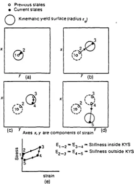
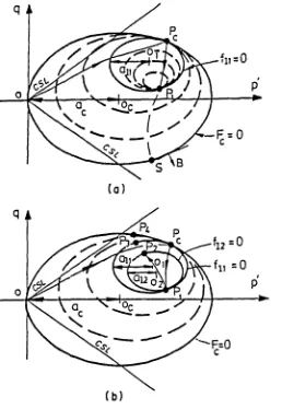
Figure 5.4.1 Diagram showing the three yield surfaces that constitute the three-surface model, defined in stress space.

Figure 5.4.2 Diagram illustrating (a) the definition of a conjugate point and the vector , (b) the geometry of the surfaces when they are in contact.

Figure 5.4.3 Diagrams illustrating (a) the definition of a conjugate point and the vector 1, (b) the geometry of the surfaces when they are in contact.

Figure 5.4.4 Diagram showing the intersection of the bounding surface or Modified Cam-clay state boundary surface with an elastic wall.

Figure 5.4.5 Diagram showing how the surfaces expand as the stress state moves to new elastic walls.

Figure 5.4.6 Diagram defining the main component of the parameters b and b2.

Figure 5.4.7 Diagram showing the position of the surfaces when b1 and b 2 are at a maximum.

Figure 5.4.8 Diagram showing how the model parameters can be obtained from typical stiffness curves for a constant q' compression path with two recent stress histories 0 degrees and 180 degrees.

Figure 5.4.9 Model predictions for an isotropic swelling stage, showing the effect of on the predicted variation in stiffness with stress change.

Figure 5.4.10 Model predictions for a constant q' compression path following two different stress path rotations. The sets of curves show the effect of on the predicted variation in stiffness with stress change.

Figure 5.4.11 Model predictions for a constant p' compression path following two different stress path rotations. The sets of curves show the effect of on the predicted variation in stiffness with stress change.

Figure 5.4.12 Model predictions for an isotropic swelling stage. The set of curves show the effect of ic on the predicted variation in stiffness with stress change.

Figure 5.4.13 Graphs illustrating the effect of (a) on the variation of stiffness with stress change for constant q' compression after a stress path reversal, (b) C' on the predicted stiffness during constant p' loading after a stress path reversal.

Figure 5.4.15 Model predictions for constant q' compression following a stress path reversal. The sets of curves illustrate the effect of (a) T and (b) T.S.

Figure 5.4.16 Model predictions for constant p' compression following a stress path reversal. The sets of data illustrate the effect of (a) T and (b) T.S.

Figure 5.4.17 Comparison between stress-strain response to failure predicted by the Modified Cam-clay model and the response predicted by the three-surface model.

Figure 5.4.18 Comparison between stress paths for one-dimensional compression, swelling and recompression predicted by the Modified Cam-clay model and the three-surface model.

Figure 5.5.1 (a) Comparison between model predictions and experimental data for constant q' compression from p -lOOkPa with p - 400kPa, 9 - 180°, (b) A sketch showing the location of the three surfaces in the model at the start of loading.

Figure 5.5.2 (a) Comparision between model predictions and experimental data for constant p' compression from p -300kPa with p - 72OkPa, 9 - 180°, (b) A sketch shoving the location of the three surfaces in the model at the start of loading.

Figure 5.5.3 (a) A comparison between experimental data and model predictions for cycles of constant p' loading at p -300kPa, p - 72OkPa, (b) A. sketch showing the location of the surfaces at the start and finish of each cycle. Figure 5.5.4 A comparison between experimental data and model

predictions for constant p' loading at Pj' - 300kPa, p - 72OkPa after four stress path rotations.

Figure 5.5.5 Plots showing the positions of the three surfaces used in the model at the start and end of each constant p' loading stage for which stiffnss data are plotted in Figure 5.5.4.

Figure 5.5.6 Model predictions of the variation in C' at Au'/to

-0.3 with stress path rotation. Data calculated for p - 300kPa, p - 72OkPa.

Figure 5.5.7 A comparison between experimental data and model predictions for constant q' compression paths after 0 degree stress path rotation, plotted as normalised bulk stiffness against p'/p

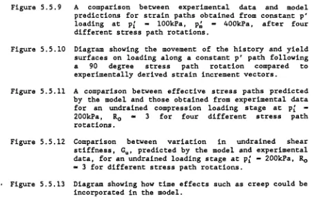
Figure 5.5.9 A comparison between experimental data and model predictions for strain paths obtained from constant p' loading at p - lOOkPa, p - 400kPa, after four different stress path rotations.

Figure 5.5.10 Diagram showing the movement of the history and yield surfaces on loading along a constant p' path following a 90 degree stress path rotation compared to experimentally derived strain increment vectors.

Figure 5.5.1). A comparison between effective stress paths predicted by the model and those obtained from experimental data for an undrained compression loading stage at p -200kPa, R0 3 for four different stress path rotations.

Figure 5.5.12 Comparison between variation in undrained shear stiffness, G, predicted by the model and experimental data, for an undrained loading stage at p' - 200kPa, R., - 3 for different stress path rotations.

ACKNOWLEDGEMENTS

The three years that I have spent at City University have been rewarding, interesting and above all great fun. I would like to thank my supervisor Prof. J. H. Atkinson for first persuading me that I would be interested in postgraduate research and then giving me so much support and encouragement during the project.

The research was supported by SERC and carried out in collaboration with Ove Arup and Partners represented by Dr B. Simpson. Dr Simpson provided several valuable opportunities for me to benefit from both his experience in the field and that of his colleagues. I am also very grateful for the interest Mr M. Gunn has shown in the project and

the comments made by Dr W. Powrie on the draft thesis.

Working at City University has been so enjoyable because of the contribution of all the other members of the research group. I would particularly like to thank Dr R. N. Taylor for all his advice and help, Dr Lewin and Mr K O'Connor for carrying out the extra experimental work that was necessary for the thesis, all the technicians but in particular Mr K. Osborne and Mr L. Martyka and, finally Dr M. Allman, Mr R. Boese, Mr K. O'Connor and Miss C. Viggiani for their helpful comments on the thesis and their friendship and assistance during the past year.

DECLARATION

ABSTRACT

The aim of the research was to study the behaviour of overconsolidated soils subjected to small changes of strain or stress appropriate to the investigation of ground movements around excavations, retaining walls or foundations, and to develop a constitutive soil model that can predict such behaviour.

The principal feature of soil behaviour investigated was the effect of recent stress history, defined by 9 the angle of rotation between the previous and current stress path directions. Stress path triaxial tests were carried out on both reconstituted and undisturbed samples of speswhite kaolin and London clay. The tests, which followed on from previous work by Richardson (1988), examined details of the influence of recent stress history, which was found to have a significant influence on the stress-strain response of the soil for the current loading path.

The data from the tests together with a re-evaluation of the existing experimental data and a limited investigation of the effect of recent stress history in 3D stress space, enabled the main features of the soil behaviour to be identified. The stress-strain response of the soil was found to be highly non-linear, inelastic and dependent on recent stress history; if the stress path rotation was 18O, i.e. a complete reversal, the soil stiffness was at a maximum and was at a minimum for no rotation. As the loading path continued the influence of the recent stress history gradually diminished until it was no longer evident. Recent stress history also affects strain paths and effective stress paths measured during drained and undrained loading respectively. The significance of mean effective pressure and overconsolidation ratio was also investigated.

LIST OF SYNBOLS

b scalar measure of degree of approach of yield surface to bounding surface - two-surface model

b 1 scalar measure of degree of approach of history surface to bounding surface - three-surface model

b 2 scalar measure of degree of approach of yield surface to history surface - three-surface model

bmax maximum value of b maximum value of b1

b 2max maximum value of b2

e void ratio

e A current value of (e + )lnp)

h0 hardening function when the current stress state lies on the bounding surface - two-surface and three-surface model

n overconsolidation ratio - general

normal to the yield surface at the current stres state-two-surface model

normal to the history surface at the conjugate stress point-three-surface model

normal to the yield surface at the current stress point-three-surface model

p' mean effective pressure

p mean effective pressure at the centre of the history surface p mean effective pressure at the centre of the yield curface p equivalent pressure: value of p at the point on the normal

compression line at the same specific volume

p mean effective pressure . at the start of the common path

the maximum mean effective pressure to which the soil has been loaded

mean effective pressure at the intersection of the current swelling line with the normal compression line

p the mean effective pressure at the centre of the yield surface - two-surface model

p, rate of change of mean effective stress

q' deviatoric stress

q deviatoric stress at the centre of the history

surface-three-surface model

q1 deviatoric stress at the centre of the yield surface - three surface model

q deviatoric stress at the start of the common path

q deviatoric stress at the conjugate stress point - three

surface model

deviatoric stress at the centre of the yield surface - two-surface model

tb0 time for 100% consolidation

V specific volume

vic specific volume of isotropically overconsolidated soil

swelled to p' - lkPa

w moisture content of the soil x, y, z cartesian coordinate axes

B Skempton's pore pressure parameter indicating the degree of saturation of the soil

Cu undrained shear strength

Young's modulus

horizontal Young's modulus for a cross-anisotropic soil Young's modulus for undrained loading

vertical Young's modulus for a cross-anisotropic soil

C, shear modulus

G* _{shear modulus in stiffness matrix derived by Craham and}

Houlsby (1983) for a transverse isotropic elastic soil G elastic shear modulus - three-surface model

C5 specific gravity

H 1 , H2 J, J K' K* Konc OCR R R0 S T p 7 E En Er Ev Es_$ S V

hardening functions - three-surface model modulus coupling shear and volumetric strains

modulus coupling shear and volumetric strains in stiffness matrix derived by Graham and Houlsby (1983) as above

bulk modulus

bulk modulus in stiffness matrix derived by Graham and Houlsby (1983)

coefficient of lateral earth pressure at rest K0 during one-dimensional normal consolidation

overconsolidation ratio defined as the maximum previous vertical effective stress divided by the current vertical effective stress

ratio of size of yield surface to bounding surface - two-surface model

overconsolidation ratio defined as p'/p

ratio of the size of the yield surface to the history surface

-three-surface model

ratio of the size of the history surface to the •bounding surface

for the two surface model, the vector joining the conjugate points on the yield and bounding surfaces; for the three-surface model the vector joining the conjugate points on the history and bounding surfaces

the vector joining the conjugate points on the yield and history surfaces - three-surface model

stress ratio, q'/p'

O angle of stress path rotation

gradient of a swelling line in mv lnp' space

- gradient of the second section of a swelling line in v : lnp' space as defined by Richardson (1988)

- gradient of the initial section of a swelling line in v lnp' space as defined by Richardson (1988)

—A gradient of the normal compression line in mv : lnp' space i.', V Poisson's ratio

&i, Poisson's ratio in cross-anisotropic soils

a' effective stress

axial effective stress radial effective stress

exponent in the hardening modulus for both two-surface and three-surface models

r specific volume of soil at critical state when p' - jkpa N specific volume of isotropically normally consolidated soil

when p' - lkPa

M critical state friction coefficient

CHAPTER 1 INTRODUCTION

1.1 Background to the Proj ect

The research described in this thesis investigates the behaviour of overconsolidated soils at small strains or small changes of stress, when the soil is far from failure. An understanding of the stress-strain response of overconsolidated soils at these stress or stress-strain levels is critical in the calculation of ground movements around excavations, retaining walls and foundations. Both Simpson et al (1979) and Jardine et al (1986) showed that the majority of the soil around structures such as these undergoes strains of less than approximately 0.2%. The development of more accurate testing techniques enabled the highly non-linear stress-strain response of the soil at these strain levels to be measured, Jardine et al (1984). Only when the behaviour of the soil at these strains is properly investigated can appropriate models be developed to predict ground movement profiles accurately.

Existing models which incorporate this non-linearity and have been used in finite element programs to predict ground movements include the largely empirical model proposed by Jardine et al (1986) and the non-linear model for London Clay described by Simpson et al (1979). The non-linear analysis carried out by Simpson et al (1979) predicted profiles of ground movements which were substantially closer to those measured in the field than predictions using linear elastic theory, thus illustrating the importance of modelling small strain stiffness correctly. Unfortunately, neither of these models incorporate all the characteristics of the behaviour of soils at small strains or changes of stress, which have been observed in laboratory tests.

derived that predict the effect not only of state and overconsoljdation ratio, but also of recent stress history. This is particularly important for civil engineering works where the recent stress history of the soil changes significantly across the construction site due to geological variations or nearby construction.

In this thesis the term recent stress history refers only to changes in direction of stress path, time effects are considered separately. The research builds on previous work at City University, primarily that described by Richardson (1988). The latter investigated the general characteristics of the recent stress history effect, for a variety of soils, through an extensive series of stress path tests on reconstituted samples.

The aims of the research reported in this thesis are as follows:

(i) To investigate recent stress history effects in more detail and hence to define the effect more clearly.

(ii) To derive and evaluate a new constitutive soil model that takes account of the influence of recent stress history.

(iii) To demonstrate that the principal features of the effect observed in reconstituted samples (Richardson, 1988) also exist in undisturbed samples.

1.2 Basic Framework

1.2.1 Basic Methodolov of the Fesearch

The general form of a constitutive equation for soil is

(6E) [C](6a') (1.2.1)

these triaxial conditions the state of the soil will be described by the stress parameters, p', q' and the specific volume, v (Schofield and Wroth, 1968), where p' - 1/3(0: + 2a), q' - - ci and v, the specific volume, is the volume in space occupied by unit volume of soil grains. Corresponding strain parameters are - + 2Er and e, - 2/3(E -

E r) .

e),

For axial symmetry, i.e. stress states in the triaxial plane, and using the stress and strain parameters given above, following Graham and Houlsby (1983) the general constitutive equation becomes.

I

_I

L Se,

L

1

(1.2.2)

-

For the particular case of a cross-anisotropic soil, J', which models the cross coupling of shear and volumetric effects, could bewritten in terms of standard anisotropic elastic parameters as follows.

J, - 3E.E1 (1.2.3)

2(E(1 -

_W

_{) -}

_"vh))

However, the coefficients of the compliance matrix in equation 1.2.2 are not necessarily elastic moduli. To develop a model which will predict the stress-strain response of the soil it is necessary to determine the functions of the soil properties, state and history which are represented by K', 3G' and J' in this equation. These functions must be consistent with the values of K', 3G' and J' calculated, as shown in section 1.2.3, from the stress-strain response measured experimentally.

history of the soil changes then tests should be carried out to obtain a new stress-strain curve and hence derive new values of K', 3G' and J'. This method has been used by Duncan and Chang (1970), who approximated the stress-strain curves to hyperbolae, and by Jardine et al (1986) to model the small strain behaviour of soils. The alternative method is to propose a conceptual model which incorporates all aspects of the soil behaviour and from which functions for K', 3G' and J' can be determined. These will be direct functions of soil properties, the stress state and model parameters which define the history of the soil, such as p in the Cam-clay model. The model would only require basic soil properties to be determined experimentally. Typical models of this type have been proposed by Al Tabbaa (1987), Mräz et al (1979) and Hashiguchi (1985).

The latter approach to modelling the behaviour of overconsolidated soils has been adopted in this thesis. The only independent variables in the new constitutive model described in Chapter 5 are soil properties. The effect of state, overconsolidation ratio and recent stress history are all included in the definition of the model. This type of model was used because, if it is installed in a finite 'element program, it will be possible to calculate the integrated effect of any number of different elements of soil loaded along different stress paths and with different states and recent stress histories all using one set of soil parameters. Depending on the complexity of the site, finite element calculations using empirical models would require considerably more sets of stress-strain data.

1.2.2 Theoretical Framework

The version of the Modified Cam-clay model which has been used as the basic framework for the new model has also been used by Houlsby et al (1982) and Al Tabbaa (1987) and incorporates the natural compression law proposed by Butterfield (1979) such that the isotropic normal compression line is given by the equation.

mv - N - Amp' (1.2.4)

where N is the value of mv when p' - 1 and A is the gradient of the line in lnv:lnp' space, as shown in Figure 1.2.1(b). This figure also shows the idealised isotropic elastic swelling line defined by

lnv - v, - iclnp' (1.2.5)

This equation not only defines the elastic volumetric strains that occur in the Modified Cam-clay model, but also any purely elastic, volumetric strain that occur in any other model proposed in this

thesis. The parameter c is not used to describe the varying gradient of experimental swelling curves. These are usually characterised by the variation of the bulk modulus, K'. The critical state line is defined in lnv:lnp' and q' :p' space respectively by the equations.

lnv - r - Alnp' (1.2.6)

and

- ± Mp' (1.2.7)

The critical state line is shown in lnv:lnp' space in Figure 1.2.1(b) and in q':p' space in Figure 1.2.1(a). States to the right of the critical state line are "wet" of critical and states to the left "dry" of critical, see Figure 1.2.1(b). This figure also shows the Modified Cam-clay yield locus, which is formed by the intersection of an elastic wall and the state boundary surface and is defined by

2

(p' -

_p

₂

perpendicular to the yield surface and is given by

____ - (P' Pc;) _(1.2.9)

&e 1 q'/ M2

An isotropic hardening law which links the expansion of the yield surface to plastic volumetric strain is given by.

6e P - (_{A - ic) 6pc;/ p} (1.2.10)

The resulting constitutive equation for the plastic strains is:

I

1

(A - ic) [(p' - Pc;)2

[8Ev j - Pc;P'( p ' Pc;) [

- Pc;) q'

-( p ' - pc;) q' 2 M4

sp' M2

6q'

(1.2.11)

1.2.3 Interp retation of Data

The basic type of test used to investigate the effect of recent stress history is described in detail in section 3.6.2. The tests examine the stress-strain response along a fixed path such a OP, in Figure 1.2.2, where the starting point 0 is approached from different directions by loading along paths such as AO and BO. The recent stress history associated with a different 'approach' path is described by the angle through which the direction of loading has to rotate to follow the fixed path. This is the angle, 9, shown in Figure 1.2.2, which is defined as positive when the rotation is in a clockwise direction. The angle of rotation, 9, is not a measure of the rotation of the principal stress directions, which are fixed in a triaxial test. The initial state of the fixed or 'common path' is described by the stress coordinates, p, q.

The majority of the test data comes from overconsolidated soils, for which the overconsolidation ratio is defined as -

ph/p'.

Cam-clay yield locus as shown in Figure 1.2.3(b). The parameter, p, is not equivalent to 2p,, defined in section 1.2.2, since for models such as those proposed in Chapter 5, plastic strains may occur inside the state boundary surface and so, unlike p, p, can decrease as well as increase.

The tests provide a series of different stress-strain curves all measured along the common path but corresponding to different approach paths. In order to obtain a clearer picture of the differences between these curves, stiffness parameters should be calculated. As noted in section 1.2.1 in the case of axial symmetry, increments of stress and strain can be related by a compliance matrix as shown below, (Atkinson and Richardson, 1985).

I 5 g ., 1 I 1/K' l/J' 1 6' 1

L 5E1 j - L 1/J' 1/3G' ] [ çq' ] (1.2.12)

where K' and G' are the bulk and shear moduli of the soil for the current increment. The modulus J' models the coupling of shear and volumetric effects (Graham and Houlsby., 1983). The majority of the

stress probe tests investigating the effect of recent stress history used drained loading paths. To isolate the moduli K' and G' two particular types of loading were used as the common path: these were loading at constant p' and loading at constant q'. For constant p' loading paths, Sp' - 0, so in the limit as the increment tends to zero

dq'/ de 1 - 3G' (1.2.13)

Hence 3G' can be defined as the gradient of a shear stress-shear strain curve obtained from constant p' loading. Similarly for constant q' loading paths Sq' - 0 and hence

dp'/ de., - K' (1.2.14)

followed during loading were also examined. These paths provide information on the nature of the deformations as described in section 4.2.5. The gradient of these paths is the strain increment ratio, de/th,, which is a measure of the anisotropy of the soil. For constant p' loading paths from equations (1.2.12)

de/d€ 1 - 3G'/J' (1.2.15)

and for constant q' loading

de/de. - J'/K' (1.2.16)

For a small number of the tests, an undrained compression stage was the common path. The cross coupling of shear and volumetric effects means that the gradient of the stress-strain curve obtained from undrained compression paths is not equal to 3G' as defined above. For undrained tests 6E, - 0, so inverting the matrix in equation 1.2.12, the value of undrained shear modulus, G, in terms of the stiffness moduli given in equation 1.2.12 is

—3G'J'2

dq'/dE - 3C - ____________ (1.2.17) (3K'G' - J'2)

The shape of the effective stress path obtained from an undrained compression test provides information on the nature of the deformations in the same way as the strain paths from drained tests. The variation in the anisotropy of the soil during the test can be measured from the gradient of the path, dp'/dq', as

dp'/dq' - —K'/J' (1.2.18)

CHAPTER 2 LITERATURE REVIEW

2.1 Introduction

This literature review examines work carried out in the three main areas of measurement, evaluation and modelling of recent stress history effects at small strains of changes of stress. In the

sections covering the development of testing techniques, and the experimental investigation of small strain deformations and recent stress history effects, the majority of the work reviewed was carried out in the laboratory, mostly using triaxial testing apparatus. This review concentrates on laboratory experimentation and apparatus because it is in this field that most of the recent work has taken place and it is from this work that the current project continues.

The development of laboratory testing techniques for measuring soil stiffness at low strain and for small stress changes was undertaken primarily in an attempt to explain the differences between stiffness moduli measured in the laboratory and moduli back calculated from field measurements. The latter were observed to be between five and ten times those derived from laboratory tests and the differences were attributed not only to deficiencies in the experimental methods used to measure stiffness in the laboratory but also to the effect on the stress-strain response of the recent stress history of the soil (Simpson et al, 1979).

2.2 Development of Experimental Techniques in Laboratory Testing

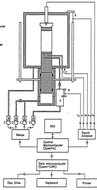
Experimental techniques used to investigate the small strain behaviour of overconsolidated soils should be able to measure stiffness moduli accurately for small changes of stress and especially at low strain levels subsequent to or during carefully selected stress paths. The major advances in laboratory test equipment and testing techniques which made these measurements possible were, firstly, the development of the hydraulic stress path cell (Bishop and Wesley, 1975) and secondly the design and use of devices to measure axial and radial strains on the sample inside the cell. In addition, equipment such as the resonant column apparatus has been used to measure stiffnesses at very small strains, less than 0.001%.

2.2.1 Develo pments in H ydraulic Stress Path Cells

The hydraulic stress path cell was developed by Bishop and Wesley (1975). The cell incorporates the feature employed by Atkinson (1973) of applying the axial load by hydraulic pressure using Bellofram rolling diaphragm seals. The sample sits on an axial ram, where it is loaded from below by fluid pressure in a chamber divided from the cell fluid by two Belloframs, one above and one below the ram. A sketch showing a cross-section of the cell is given in Figure 2.2.1. The standard Bishop and Wesley cell for 38mm diameter samples was developed into a cell which can accommodate samples in excess of 100mm in diameter by Atkinson et al. (1984).

(1983) used continuous motors, automatically controlled by a microcomputer, to control manostat air pressure regulators. Two subsequent modifications to this system substituted, first electromanostats for the motor driven pressure regulators (Atkinson, 1985) and, secondly, analogue pressure converters, (Viggiani, 1990).

The hydraulic stress path cell was developed so that soil deformation parameters could be measured over a wide range of stress paths. Lewin and Burland (1970) and Davis and Poulos (1968), among others, recognised that stiffness measured directly from a triaxial test is dependent on the stress path followed by the soil. Therefore, appropriate deformation characteristics would only be obtained if the appropriate stress path was followed. To conduct stress path tests in conventional triaxial cells the axial load is applied by dead weights and can only be increased in steps. This means that it is almost impossible to follow any stress path other than conventional triaxial compression or extension. A Bishop and Wesley hydraulic stress path cell operated by any of the control systems described here will enable the appropriate stress history of the soil, such as I( compression or swelling, to be followed with reasonable accuracy.

2.2.2 Develo pments in Strain Measurin Techniques

There are three main areas in which strain measuring techniques have been improved and developed. Firstly, errors in externally made measurements have been eliminated using special procedures and relatively simple modifications to existing testing apparatus. Secondly, methods of measuring strains local to the sample have been developed, in particular internal strain transducers mounted on the sample. Thirdly, laboratory testing apparatus that can measure very small strains, less than 0.001%, have been developed.

top platen beds into the sample. The accuracy of the axial strains measured in this way was estimated as ±0.01%.

A considerable number of different approaches to the problem of measuring local axial strains have been developed. A comprehensive review of the early work in this field is given by Costa Filho (1985). The different types of procedure that have been used include X-ray techniques to measure the movement of lead shot set in the sample (for example Balasubramaniain (1976)) and a pair of cathetometers sighting on inscribed drawing pins stuck into the sample below the membrane (Atkinson, 1973).

Initial attempts to measure local axial and radial strains by mounting transducers on the sample were made using miniature LVDTs (for example Brown and Snaith, 1974). Costa Filho (1985) continued with this system and described a set up using two miniature LVDTs to measure strains over a gauge length of approximately 25mm on samples of overconsolidated London Clay, see Figure 2.2.2. The accuracy of measurements made at low strains was estimated as ±0.005%.

There are two further methods of measuring local strains which have been used recently. The first, designed by Clayton and Khatrush (1986) and Clayton et al. (1989), made use of Hall effect semiconductors which operate by detecting changes in magnetic flux. The device is in two halves: the semiconductor and its mounting are fixed to the sample at one end of the gauge length and the magnet causing the changes in magnetic flux is on an arm fixed to the other end of the gauge length. Figure 2.2.5 shows this configuration, which is used to measure axial strains, and also a radial strain measuring device based on a Bishop and Henkel (1962) lateral strain caliper. Clayton and Khatrush (1986) reported that the gauges were temperature and voltage stabilised and capable of measuring axial strains to 0.002%. The second technique for measuring local strains was described by Hird and Yung (1987) who used proximity transducers to measure local strains on 100mm diameter samples with an accuracy of 0.009% for strains less than 0.1%.

It is particularly important to measure strains with gauges attached to the sample when testing stiff overconsolidated clays. At low stress levels the strains are very small, often less than 0.1%, and so inaccuracies in measurements made using a transducer mounted outside the cell will be significant. Jardine et al. (1984) and Clayton et al. (1989) identified a number of errors in external measurements such as load cell deflection and bedding and tilting of the sample. A diagram of a typical sample in a triaxial cell showing the exact origin of the errors identified by Jardine et al. (1984) is given in Figure 2.2.6. Both this paper and the paper by Clayton et al. (1989) concluded that these errors were the primary cause of the observed difference between field and laboratory measured stiffness moduli. However, the errors can be largely eliminated using the procedures given by Atkinson and Evans (1985) who felt that the increased accuracy obtained by measuring axial strains locally compared with external strains measured following their guidelines, was principally due to the greater resolution of the equipment.

importance of end restraint and bedding errors and, for samples of undisturbed London clay, found that, although end restraint effects would cause the stiffness to be somewhat overestimated, bedding errors were more significant.

The equipment used most couunonly to measure shear stiffness at strains of less than 0.001% in the laboratory is the resonant column apparatus. Three types of test can be carried out using the resonant column to obtain values of the shear modulus of the soil. These tests are the resonant column test, the free vibration decay test and the cyclic torsional shear test. The original resonant column test (Richart et al., 1970) loaded a cylindrical sample, or column, of soil dynamically in torsional shear at a given amplitude but varying frequency. The shear modulus of the soil was calculated by comparing the response of the soil when resonance occurred to a theoretical model. Current resonant column testing methods employ all three types of test in a multistep technique (Isenhower, 1979).

The main alternative method of measuring these very small strain stiffness moduli in the laboratory was described by Schulteiss (1981) The technique used piezoceramic crystals, known as bender elements, to send pulse shear waves through a triaxial sample which were picked up by a further bender element acting as a sensor at the top of the sample. The shear modulus of the sample was calculated from the velocity of the waves obtained by measuring the time for the wave to pass between the two sensors.

Dynamic testing methods appear to be the only means of resolving strains of 0.001% or less in the laboratory. Recent work by Ranipello (1989) testing Todi clay indicates that, at equivalent shear strains, dynamic stiffness moduli obtained from resonant column tests and static stiffness moduli measured in triaxial tests using local axial strain gauges are comparable. However, it should be noted that the loading path and recent stress history of soil subjected to dynamic testing are always the same and are equivalent to a series of unload-reload loops.

and the appropriate overall and recent stress history of the soil to be recreated. Improved techniques of measuring strains, especially the use of local axial strain gauges in triaxial cells, means that this stress-strain response can be determined for strains as low as 0.001%. The shear stiffness of the soil can be obtained at lower strain levels using apparatus such as the resonant column or bender elements but these moduli are only applicable to the limited stress path and recent stress history provided by dynamic loading.

2.3 Experimental Investigation of Deformations at Small Strains

As noted in the previous section, experimental techniques enabling stress-strain relationships for overconsolidated soils to be determined at low stress levels and small strains have only been developed relatively recently and this section will concentrate on the comparatively limited selection of data obtained using these procedures.

The work in this area falls into two main categories.

(i) Experimental work concentrating on the accurate measurement of the small strain stiffness of soils.

(ii) The experimental evaluation of the effect of recent stress history.

The results of work carried out to fulfill the first category also provided data on the effect of recent stress history on soil behaviour although the tests were not specifically designed for this purpose.

The non-linear stress-strain response of overconsolidated soils was reported by Costa Filho and Vaughan (1980) for London Clay and Jardine et al (1984) and Jardine (1985) for a variety of soils but predominantly London Clay and a low plasticity North Sea clay. Costa Filho and Vaughan (1980) described results from unconsolidated undrained and anisotropically consolidated undrained tests on samples of London clay. During the tests local axial strains were measured using the method given in Costa Filho (1985). The stress-strain response of the London Clay in both tests was highly non-linear. In addition the anisotropically consolidated undrained tests showed an initial stiffness which was greater than that observed in the undrained tests on unconsolidated samples, see Figure 2.3.1. Costa Filho and Vaughan (1980) and Costa Filho (1979) concluded that in comparing the stiffness of overconsolidated soils, such as London Clay, it is necessary to account for both the strain level and stress history of the soil.

Jardine (1985) reached similar conclusions from the results of an

extensive series of tests on reconstituted samples of a low plasticity

North Sea clay. All the tests were undrained but different stress histories and reconsolidation procedures were followed before the compression or extension shearing stage. Electrolevel internal strain gauges were used to measure the highly non-linear stress-strain response of the soil. This non-linear stress-strain response was characterised using an initial secant Young's modulus, when the axial strain was 0.01%, and a non-linearity index or a non-linearity function. For the one-dimensionally consolidated soil the non-linearity function was found to depend both on preshearing conditions, i.e. the stress history of the soil, and the length of time that the soil was held at the current stress state, and the loading direction.

plotted on a set of typical stress paths. The previous stress history of the soil appeared to affect the size and shape of the zones.

The observation was also reported in Jardine et al (1984) and Hight et al. (1985). Night et al. (1985) identified a region or zone bounded by strains of 0.01% in order to explain the behaviour of soil after different stress paths and histories during sampling. If the current stress path was a continuation of the previous path the zone was hardly traversed at all and the initial stiffness observed was lower.

If there was a stress reversal the zone was traversed completely and there was an increase in stiffness. There was also some indication that the zone decreased in size as the soil swelled back from a normally consolidated state.

It should be noted that none of the results that have been reviewed above isolate the influence of recent stress history. Where differences in the stress-strain behaviour of the soil have been attributed to the influence of previous stress history, the stress history referred to is not necessarily only recent stress history as stress state and overconsolidation ratio have also been altered. Although the zones of different behaviour identified by different strain levels provide a useful method of monitoring the variation in stress-strain response of the soil, they cannot be used to explain this stress-strain behaviour which was itself used to define them.

Clinton (1987) carried out a series of stress probing tests on samples of Cault clay in order to determine anisotropic stiffness moduli. The results of the tests implied that the soil had different stiffness parameters for the same stress state and overconsolidation ratio when the probe was preceded by different recent stress histories. In this case the effect of recent stress history was isolated from the effect of state or overconsolidation ratio.

for shear strains of less than 0.001%. Rampello (1989) testing Todi clay also established from tests using a resonant column apparatus, similar to that used by Isenhower (1979), that the shear modulus is at a maximum and constant for strains less than 0.001%. Ranipello (1989) used both undisturbed samples and samples which as part of their previous stress history had been swelled back to very low effective stresses. Both types of sample were tested at a number of different initial stress states. The results of these tests are shown in Figure 2.3.3 as shear modulus normalised by the initial maximum shear modulus against strain amplitude. The variation of the normalised shear modulus is approximately constant for all the tests. The general form of this curve is typical of many results of resonant column tests on clays (see Sun et al. (1988)).

Rampello (1989) also compared the moduli observed from the resonant column tests directly with corresponding moduli obtained by using electrolevel gauges to measure local axial strains during triaxial undrained shear tests. The data compare well as shown by Figure 2.3.4 which shows the data plotted as the variation of Young's modulus with axial stress.

These results clearly confirm the highly non-linear stress-strain behaviour of overconsolidated clays at strains greater than 0.001%. However it is difficult to draw any conclusions about the importance of recent stress history because the two tests impose different stress conditions on the sample and the recent stress history of the triaxial samples is not always clear.

There have been very few laboratory test programs specifically aimed at investigating the effect of recent stress history on the stress-strain behaviour of overconsolidated soils. However, Som (1968) testing London Clay reported that if a sample was held at a constant stress state in an oedometer for many days before a new load increment was applied, the stiffness for that load increment was increased provided that the increment was small. This illustrated the effect of rest period on the subsequent stiffness of soil.

in undrained compression from the same stress state and overconsolidation ratio. However, one pair had been anisotropically and the other isotropically consolidated and swelled. In addition, for both pairs one sample was swelled back past the initial state for the shearing stage and recompressed back. The other sample was only swelled to the initial state and sheared. Both the samples which had been subjected to a recompression cycle before shearing showed a much less stiff stress-strain response. The undrained effective stress path followed by these two samples was also affected by the recompression stage but the different overall stress histories, i.e. isotropic or anisotropic, of the soil appeared to have a more significant influence.

The most important series of tests used to study the effect of recent stress history on the stress-strain behaviour of overconsolidated soils was completed by Richardson (1988). A comprehensive program of drained stress path tests on reconstituted samples of speswhite kaolin, London clay, Cowden Till, Ware Till and slate dust was carried out. The stress probes followed during the tests isolated the effect of recent stress history for soils subjected to different overall stress histories such as one-dimensional consolidation and swelling. Various overconsolidation ratios and time effects were also investigated. Combinations of stress probes were frequently duplicated to ensure that the results were repeatable. Richardson (1988) found that the recent stress history of a soil has a significant effect on both the stiffness of a soil and its stress induced anisotropy. The results of this work form the basis of much of the work in this thesis and are reviewed in more detail in section 4.3. A selection of the data obtained from the tests on London Clay is described by Atkinson et al. (1990). A typical set of data obtained from an investigation of the effect of recent stress history on the stress-strain response of an overconsolidated sample of London clay for a constant p' loading is given in Figure 2.3.5.

the dependence of stiffness on recent history, but only for strain levels greater than 0.01%. The results of the undrained tests by Jardine (1985) and the resonant column tests by Rampello (1989), among others, give a more extensive picture of the non-linear stress-strain behaviour and identify an elastic region of soil deformation at strains of less than 0.001%. Unfortunately it is not easy to quantify the effect of recent stress history on this behaviour from these latter tests.

2.4 Soil Models for the Stress-Strain Behaviour of Overconsolidated Soil

This section reviews existing continuum numerical models which have been formulated to predict the stress-strain behaviour of fine grained soils at states lying within the state boundary surface. The majority of the models reviewed in this section were originally defined in general stress space and then modified to model the specific case of soils tested in triaxial stress conditions. As most test data is obtained from triaxial tests it is simpler to evaluate the model in this form. The models can be divided into two groups.

(i) Models which assume all deformations inside the state boundary surface are elastic.

(ii) Models which allow plastic yielding to occur inside the state boundary surface.

2.4.1 Elastic Models

-E'/2(l-i-v'), and the bulk modulus K' - E'/3(l-2u'). Using the stress

and strain invariants p', q', €,, and e 5 , the matrix equation relating

increments of stress and strain for an isotropic elastic soil is;

K' 0 6€,

- (2.4.1)

Sq' 0 3G' 6€

The isotropic linear elastic stress-strain behaviour represented by

this equation has been used extensively to predict ground movements

around structures constructed in stiff clays, (e:g. Davis and Poulos,

1968).

A simple form of nonlinear isotropic elasticity was incorporated in

the Cain-clay critical state soil model formulated by Schofield and

Wroth (1968). The model can undergo recoverable volumetric strains

inside the state boundary surface but not recoverable shear strains.

The state boundary surface for Cam-clay was derived by assuming a

balanced energy equation. Introducing recoverable shear strain would

alter the state boundary surface. The elastic volumetric strains were

defined by the relationship 6€ - —Sv/v Sp'/vp'. Hence the

incremental bulk modulus, K' given in equation 2.4.1 is vp'/sc and C'

is infinite. The Modified Cam-clay model (Roscoe and Burland, 1968)

used the same definition of elastic stress-strain behaviour.

Atkinson and Bransby (1978) proposed that a more realistic model for

the elastic deformation of soil would be obtained by assuming that C'

was not infinite but varied with mean effective stress in the same way

as K'. Thus C' — K'[3(l-2u')/2(l+u')] where u' is a constant. The state boundary surface derived in the Cam-clay model was not modified.

Experimental evidence that G' is dependent on the mean effective

pressure had previously been provided by Wroth (1971), who analysed

data from tests on undisturbed samples of London clay carried out by

Webb (1967). Wroth (1971) concluded that the parameters K' and G' in

a model of the elastic stress-strain response of the soil should be

determined primarily by p' and to a lesser degree by overconsolidation

ratio. The overconsolidation ratio could be represented by the

parameter e, where e A - e + Alnp'. These experimental data also

Zytinski et al. (1978), examining the thermodynamic implications of an elastic model where G' varied with p' while Poissons ratio remained constant, found that it was not conservative which is a condition for elastic behaviour. However, the alternative assumption, that Poissons ratio varied and G' was a constant, resulted in negative values for Poissons ratio, which were clearly unreasonable. The only remaining option was to abandon the idea of a purely elastic model for soil behaviour.

As reported above, in the critical state soil models elastic volumetric strains occurring during the swelling and recompression of

the soil are modelled by assuming that the specific volume of the soil varies linearly with the logarithm of the mean effective stress. As an alternative Butterfield (1979) proposed that the logarithm of the specific volume should be related to the logarithm of the mean effective stress state. For overconsolidated soils the most significant advantage of this "natural compression law" is that natural volumetric strains, as defined in section 1.2.1 are linked directly to the logarithm of the stress change. For isotropic elastic behaviour, Se,, - (,c'/p')Sp', or K' - ic'/p'.

All the above models assume that soil can be modelled as isotropic elastic although for many natural soils it is more realistic to use an anisotropic elastic model. The most appropriate form of anisotropy assumes that the soil has a vertical axis of symmetry and is known as cross-anisotropy or transverse isotropy. Love (1942) established that five independent parameters were required to define the behaviour of a transversely isotropic soil and the various thermodynamic limits on the values of these five parameters were investigated by Pickering

(1970) and Gibson (1974). Graham and Houlsby (1983) provided a matrix equation for a transverse isotropic elastic soil in terms of triaxial stress invariants.

[

rK* _Ji

(2.4.2)

'1

L3i