Development of a variance prioritized multiresponse robust design framework for quality improvement

Development of a variance prioritized multiresponse

robust design framework for quality improvement

Jami Kovach

Department of Information and Logistics Technology, University of Houston, Houston, Texas 77204, USA

Byung Rae Cho

Advanced Quality Engineering Laboratory, Department of Industrial Engineering, Clemson University, Clemson, South Carolina 29634, USA

Jiju Antony

Strathclyde Institute of Operations Management, Design Manufacturing and Engineering Management, University of Strathclyde, Glasgow, G1 1XY, UK

Submitted to:

International Journal of Quality and Reliability Management

February 2008

Development of a variance prioritized multiresponse

robust design framework for quality improvement

Jami Kovach

Department of Information and Logistics Technology, University of Houston, Houston, Texas 77204, USA

Byung Rae Cho

Advanced Quality Engineering Laboratory, Department of Industrial Engineering, Clemson University, Clemson, South Carolina 29634, USA

Jiju Antony

Strathclyde Institute of Operations Management, Design Manufacturing and Engineering Management, University of Strathclyde, Glasgow, G1 1XY, UK

Abstract

Purpose – Robust design is a well-known quality improvement method that focuses on building quality into the design of products and services. Yet, most well established robust design models only consider a single performance measure and their prioritization schemes do not always address the inherent goal of robust design. In this paper, we propose a new robust design method for multiple quality characteristics where the goal is to first reduce the variability of the system under investigation and then attempt to locate the mean at the desired target value.

Design/methodology/approach – In this paper, we investigate the use of a response surface approach and a sequential optimization strategy to create a flexible and structured method for modeling multiresponse problems in the context of robust design. Nonlinear programming is used as an optimization tool.

Findings – Our proposed methodology is demonstrated through a numerical example and the results are compared to that of the traditional robust design method. The proposed methodology provides enhanced optimal robust design solutions consistently.

Originality/value – This paper is perhaps the first study on the prioritized response robust design with the consideration of multiple quality characteristics. The findings and key observations of this paper will be of significant values to the quality and reliability engineering/management community.

Keywords Quality, robust design, multiresponse problems

Introduction

In today’s industrial production environment, it is essential that companies create and retain a

competitive advantage over their competitors with respect to quality in order to be successful.

The robust design (RD) methodology, first developed by Taguchi (1986, 1987), is important to

industrial quality improvement initiatives. This approach focuses on building quality into the

design of products and services though the determination of the optimum operating conditions in

order to minimize performance variability and deviation from the target value of interest (i.e.

process bias). Since it was first introduced, this approach has come under serious criticism due to

the statistical analysis methods and optimization approaches utilized. In his method of RD,

Taguchi advocates minimizing signal-to-noise ratios to determine the best overall combination of

design parameter settings and identifying adjustment factors, which are used to adjust the mean

to the desired target value. Yet, Nair and Shoemaker (1990) argue that by simply collapsing

experimental data into signal-to-noise ratios much of the information concerning the system’s

behavior is lost. Additionally, Taguchi gives no real justification for the use of these ratios, and

the details surrounding the use of adjustment factors to achieve the target value of interest are

sketchy at best. To address these issues, there have been several attempts in the literature to

improve the analysis and optimization phases of the RD methodology.

Several RD optimization models that are relevant to the work presented here are based on

the dual response approach, which was first considered by Myers and Carter (1973). Here, the

process mean and variance of a single quality characteristic are modeled separately using

response surfaces. These functions are then optimized simultaneously to determine the system’s

optimum operating parameters. The first attempt to combine this type of optimization model

dual response approach to RD, Lin and Tu (1995) proposed the mean-squared error (MSE)

model. This approach relaxed the zero-bias assumption of the previous model to provide

solutions that are better (or at least equal), in terms of the variance achieved, through a more

flexible optimization model. Lin and Tu (1995) further suggested assigning different weights to

process bias and variability as a way of prioritizing the optimization procedure. Along these

lines, Park and Cho (2003), Shin and Cho (2005), and Cho and Park (2005) considered more

complex RD systems from the viewpoints of non-normal data, process oriented modeling, and

unbalanced design space, respectively, Finally, Kovach and Cho (2006) and Lee et al. (2007)

developed RD models for unbalanced data structures and irregular experimental situations,

respectively.

The RD optimization models discussed thus far may be considered multiresponse

approaches because they simultaneously optimize the response models for both the process mean

and variance. These approaches, however, only consider the response models for the process

mean and variance for a single performance measure. Yet, customer judge products on multiple

scales simultaneously. Further, the prioritization scheme of these optimization models do not

always address the inherent goal of RD. Taguchi (1986, 1987) believed it was vital to quality

improvement efforts to not simply focus on adjusting the process mean to the desired target

value. He felt strongly that it was also critical to reduce the variability of the process around the

mean. Therefore, when optimizing a system, RD should consider multiple quality characteristics

simultaneously and place top priority on minimizing process variability. In this paper, we

propose a new approach to the multiresponse RD problem to address these issues, called

variance-prioritized multiresponse robust design (VPMRD). In this approach, the optimization

scheme is specified using a preemptive optimization procedure. Through a numerical example,

we demonstrate the use of this methodology to determine the optimum operating conditions for

the system under investigation based on experimentation and system modeling.

In the next section, we describe our proposed methodology in detail. Then, an example is

used to demonstrate the practical implementation of our proposed approach. Next, a comparison

study is conducted to validate the proposed model. Finally, we discuss conclusions concerning

the practical implications of the proposed approach.

The proposed methodology

While there are several optimization models that can be employed within the RD methodology,

few consider the inherent goal of RD. Recall that Taguchi’s quality philosophy suggests that

quality improvement efforts should not simply focus on the mean; it also involves the variability

around the mean. Yet, well-established optimization approaches, including the dual response

(Vining and Myers, 1990) and MSE models (Lin and Tu, 1995), may have failed to place top

priority on minimizing the variance. Therefore, we propose a new method of RD that creates a

structured, yet flexible modeling approach for multiresponse RD problems where the goal is to

first reduce the variability of the system under investigation and then attempt to reduce the

process bias. In this new approach, we utilize nonlinear goal programming techniques [3] to

determine the system’s optimum operating conditions based on response surface models of the

system derived though experimentation and analysis.

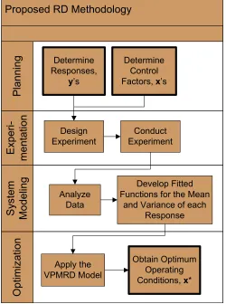
The methodology proposed in this paper is shown in Figure 1, which consists of first

determining the problem to be considered and choosing the responses of interest, as well as the

appropriate experimental design, and the experiment is carried out according to plan. Next, data

collected from the experiment are analyzed using the least squares method of regression analysis.

Based on these results, response surface models for the mean and variance of each response are

created. Finally, the proposed VPMRD model is used to simultaneously optimize the responses

to obtain the settings for the design parameters that make the system under investigation perform

optimally relative to minimizing the process’ variance and bias.

[Figure 1 Approximately Here]

Planning

In an RD study, the determination of the quality characteristics of interest is strongly related to

the nature of the problem being investigated. Similarly, the choice of experimental parameters is

often derived from the responses under investigation using prior engineering knowledge

concerning the system being studied. In many situations, however, practitioners may not have

sufficient experience to effectively choose the appropriate experimental parameters. Therefore,

the alternative is to collect data relative to potential experimental factors and then use

multivariate studies, correlation analysis, and/or screening experiments to determine the specific

factors to consider in an RD investigation.

Experimentation

In designing an experiment, there are many standard approaches from which to choose. These

include, but are not limited to, factorial designs, Taguchi designs, and response surface designs.

The key, therefore, is to choose the design that best addresses the experimental question and

supports the desired data analysis given the available resources (i.e. time and experimental

number of levels of each factor to be tested, and the number of replications planned. The results

obtained form the experiment provides the information necessary to create response surface

models that describe the behavior of the system under investigation.

System modeling

To create response surface models for the mean and variance of each quality characteristic under

investigation, we utilize the least squares method of regression analysis. Using this approach,

consider that each of the n treatment combinations in an experiment consists of r replicates. For each response of interest, let yuj represent the jth response at the uth treatment where

1 2

j= , , , r and u=1 2, , , n. Then, for each quality characteristic, the mean and variance for

the uth treatment can be estimated using the following equations:

(

)

1 2 1

and

1

r r

uj uj u

j j

u u

y y y

y s

r r

= = −

= =

−

∑

∑

(1)

for u=1 2, , , n. Assuming the underlying distribution of the experimental data is normal with

constant variance, the estimators given in Equation (1) are then used to create the response

surface functions of the mean and variance based on the method of least squares regression

analysis as follows. The model for the mean, therefore, is written as

( )

µ

∧ ∧

=

x Xβ, (2)

where

(

)

∧ ₋

=

X is the design matrix, β∧ is the estimate of the vector of unknown model parameters, and y is

the vector of estimated means for each treatment combination in an experiment. In addition, the

response surface function for the variance is given as

( )

∧

=Xγ

x

2

σ , (4)

where

(

)

∧ ₋

=

γ X X X s , (5)

∧

γ is the estimate of the vector of unknown model parameters, and 2

s is the vector of estimated

variances for each treatment in an experiment. However, if the underlying distribution of the

experimental data is skewed (i.e. is significantly non-normal) or the assumption of constant

error-variance is violated significantly, the data will have to be transformed in order to proceed

with this type of analysis. Commonly used transformations include, but are not limited to, a log

transformation or square root transformation; the transformation to be used depends on the

specific situation and the degree to which the necessary assumptions are violated. Assuming the

necessary assumptions can be verified, the fitted response functions for each quality

characteristic under investigation are then optimized simultaneously to determining the system’s

optimum operating parameters.

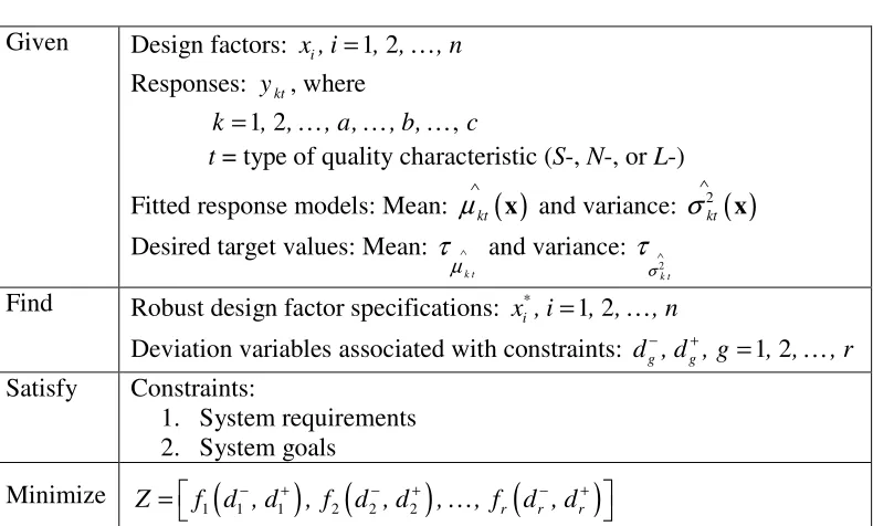
Optimization

The framework for the proposed optimization model is shown in Table 1 and is structured

in such a way that given the system parameters and the models of their behavior, the goal is to

find the design factor settings based on satisfying the system requirements and goals by

These designations are necessary to accommodate the different types of quality characteristics

that may be considered in an RD investigation. According to Taguchi, responses are usually

categorized as one of the following three types.

1. Smaller-the-better (S-type): Minimize the quality characteristic of interest (i.e. the target value equals zero).

2. Nominal-the-better (N-type): The quality characteristic of interest has a specific target value.

3. Larger-the-better (L-type): Maximize the quality characteristic of interest (i.e. the target value approaches infinity).

Further, µ_kt

_{( )}

∧

x and σ2_kt

_{( )}

∧

x are the response surface functions for the process mean and

variance of response ykt, respectively, which are assumed to be independent of each other, and

k t

µ

τ ∧ and

2

k t

σ

τ ∧ are the desired target values for the mean and variance of response ykt,

respectively.

[Table 1 Approximately Here]

In the proposed model, the constraints consist of the system’s technical requirements and

its desired goals. The system requirements are characterized by the upper and/or lower limits on

the system variables under consideration, which must be satisfied in order for the solution to be

feasible. Further, the constraints representing the system goals model the deviation from the

desired target values for both the mean and variance of each response. Overall, the system goal is

to minimize the deviation from the desired target values. Additionally, we can specify the

priority of individual goals in the objective function given this framework.

The objective function for the proposed model is formulated as a nonlinear goal

programming problem (Hillier and Liberman, 2001). This type of approach makes the general

as a single function using deviation variables. In mathematical programming terms, deviation

variables are also known as auxiliary variables. In the objective function for our proposed model,

these variables are used to denote the under- and over-achievement of a constraint (i.e. a desired

range or target value), which are given as dg and dg

− +

, respectively; hence, the deviation

variables are also used in formulating the constraints for the proposed model. For example,

consider the constraint associated with the process mean of a particular response of interest.

Using deviation variables, this constraint can be written in general terms as

_{( )}

k t

g kt d

µ

µ τ ∧

∧

= x − , for g=1 2, , , r (6)

where

g g g

d d+ d−

= − (7)

and

{

0 otherwise

if 0

0 otherwise g g g g g g d d d d d d + − ≥ =  _≤ =  (8)

Given these definitions, the constraint in Equation (6) can then be rewritten as

( )

(

)

k t

kt dg dg

µ

µ τ ∧

∧

+ −

− − =

x . (9)

Further, the method described here for modeling constraints using deviation variables for the

mean of a quality characteristic can also be used for modeling the variance. Given this type of

approach, the deviation variables associated with the constraints for the mean and variance of

each response are then combined to form a single objective function as follows:

min Z f d , d1

(

)

(

)

(

)

− + − + − +

 

=_{ } (10)

1. S-type quality characteristic: µkS

( )

∧

≤

x for k=1 2, , , a

2. N-type quality characteristic: LSL_kN µ_kN

_{( )}

∧

≤ x ≤ for k=a+1, a+2, , b

3. L-type quality characteristic: µ_kL

_{( )}

∧

≥

x for k= +b 1, b+2, , c

Constraints due to system goals: 1. Process mean:

( )

k t

kt dg dg

µ

µ τ ∧

∧

− +

+ − =

x for t = type of quality characteristic (S-, N-, or L-) 2. Process variance:

( )

2

2

k t

kt dg dg

σ

σ τ ∧

∧

− +

+ − =

x for t = type of quality characteristic (S-, N-, or L-) Bounds:

1. Design factors: ximin ≤xi ≤ximaxfor i=1 2, , , n

2. Deviation variables: −, +≥0

g g d

d and −⋅ + =0

g g d

d for g=1 2, , , r

In the proposed model, the constraints are delineated according to the type of quality

characteristic considered where USL and LSL are the upper and lower specification limits,

respectively, for the system’s requirements. To establish a prioritization scheme for the

optimization procedure, our proposed model utilizes a preemptive approach involving sequential

optimization. Here, weights of different magnitudes are assigned to the deviation variables

associated with the process mean and variance. In this model, we propose setting priorities in

such a way that the goal is to first minimize the variance and then attempt to achieve the mean

equal to the desired target value. The proposed approach is illustrated through the numerical

example in the following section.

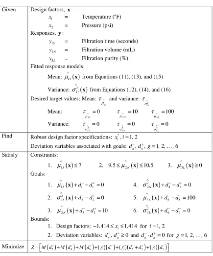
Implementation of the proposed model

Consider the problem of optimizing a chemical filtration process for measuring dosages with

respect to filtration time, volume, and purity. Here, we consider temperature (x1) and pressure

(y_3L) as our responses of interest. Hence, this becomes a multiresponse RD study, given that

there are multiple quality characteristics of interest in determining the optimum operating

conditions for the system under investigation. In this example, filtration time is considered an S -type quality characteristic since it is desirable to minimize processing time. Additionally, the

system configuration has a maximum processing time of 7 seconds that cannot be exceeded. The

desired target for the volume of the filtered chemical dose is 10 mL, where the allowable

tolerance is ±0.5 mL; therefore, filtration volume is considered an N-type response. Further,

filtration purity is required to be as high as possible, therefore this response is considered an L -type quality characteristic with a natural bound at 100%. In this particular example, it is critical

that we reduce the variability of each response simultaneously in order to stabilize the processing

cost in terms of filtration time and improve product quality by minimizing the occurrence of

under- and over-filled vials and stabilizing filtration purity.

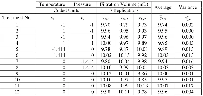
To estimate quadratic models of the responses, a central composite design with four

center points is chosen for this experiment. Additionally, the experiment is replicated three times

and data are collected concerning the responses of interest. The experimental design schemes and

the data for each response are displayed in Tables 2-4, respectively.

[Table 2 – Approximately Here]

[Table 3 – Approximately Here]

[Table 4 – Approximately Here]

Analysis of the data, using the method shown in Section 2.3, results in response surface

models for the mean and variance of each response as follows:

( )

1S 2 1725 0 1913. - . x - .1 0 1470x2 0 0613. x - .1 0 1163x - .2 0 2375x x1 2

( )

2 2 2

1S 0 03300 0 0004. - . x - .1 0 0008x - .2 0 0154x - .1 0 0151x2 0 0013. x x1 2

σ

∧

= +

x (12)

( )

2N 10 0000 0 0497. . x1 0 0434. x - .2 0 0381x - .1 0 0256x - .2 0 055x x1 2

µ∧ x = + + (13)

( )

2 2 2

2N 0 0058 0 0001. . x - .1 0 0022x2 0 0011. x - .1 0 0006x2 0 0013. x x1 2

σ

∧

= + + +

x (14)

( )

3L 94 9775 0 4832. . x1 0 7465. x - .2 0 3725x - .1 0 3175x2 0 1550. x x1 2

µ∧ x = + + + (15)

( )

2 2 2

3L 0 1898 0 0011. - . x - .1 0 0039x - .2 0 0942x - .1 0 0902x2 0 0013. x x1 2

σ

∧

= +

x (16)

Using Equations (11) through (16), the proposed VPMRD optimization model is then

applied to obtain the optimum operating conditions for the filtration process, as shown in Table

5. In this particular example, the constraints are comprised of the bounds on the responses that

must be strictly adhered to. These bounds are denoted by the technical requirements of the

system stated as the USL and/or LSL. Specifically, filtration time must be less than 7 seconds,

filtration volume must be within the range of 9.5-10.5 mL, and filtration purity must be greater

than zero. Further, the goals are determined based on the desire to minimize the process bias and

variance. For this example, the target values of interest are theoretically zero seconds for

filtration time, 10 mL for filtration volume, and 100% for filtration purity. Additionally, we

specify that the target for the variance is equal to zero because the goal of an RD study is always

to minimize the variance. Given these constraints and their associated deviation variables, the

deviation function to be minimized considers the over-achievement for the S- and N-type quality characteristics and the under-achievement for the N- and L-type quality characteristics of interests for the mean and the over-achievement of each quality characteristic for the variance.

Here, the streamlined procedure for preemptive goal programming is used to first minimize the

responses of interest are weighted equally. The big M method [3] is utilized to establish a

prioritization scheme within the optimization process. Here, the deviation variables associated

with the variance are given substantially larger weights, designated by M, over that of the

deviation variables associated with the process bias.

[Table 5 – Approximately Here]

The results of the proposed method, which are shown in Table 6, indicate the goal of zero

variance for filtration purity was achieved; yet, the variance of both filtration time and volume

slightly exceed zero. In addition, the mean of each response is achieved with minimal amounts of

bias allowed; however, none of the mean values achieved the exact target value desired.

[Table 7 – Approximately Here]

Comparison study

In this section, we validate the proposed methodology by comparing its results to those obtained

using traditional RD optimization models, including both the dual response approach (Vining

and Myers, 1990) and the MSE model (Lin and Tu, 1995). The dual response approach

minimizes the variance with the constraint that the process mean equals the desired target value,

which can be written as

min σ2

( )

∧

x (17)

s.t. µ

_{( )}

∧

= x ∈ x

where is the region of interest. This optimization model is typically used for problems in

value. Given this approach, we obtain optimum operating conditions that result in the mean

located on target with some amount of variation around the mean.

To improve upon the dual response approach, Lin and Tu (1995) relaxed its zero-bias

assumption (i.e. the constraint requiring that the process mean must equal the desired target

value) and proposed a model that simultaneously minimizes the squared difference of the mean

from the target value and the variance as follows:

min

_{( )}

_{( )}

2 2

+

µ τ σ

∧ ∧

 

−

 

 x  x (18)

s.t. x∈

When minimizing the variability of the response of interest is of equal or greater importance than

achieving the desired target value, this optimization strategy is often utilized. Based on such an

approach, it is observed that by allowing some difference between the mean and the desired

target value, the resulting process variance is less than or at most equal to the variance of the

dual response approach.

For the purpose of comparison, we utilize an approach similar to that demonstrated by

Tang and Xu (1995) in which we approximate the traditional RD models using the VPMRD

framework developed in this paper. Here, we reformulate the original RD models as goal

programming problems and apply them to the example used previously to illustrate our proposed

methodology. The formulations of and the results obtained from these equivalent models are

presented in the following sections. The results obtained using these models are then compared

to the results obtained from our proposed methodology.

Using the dual response approach, the first priority of the optimization procedure is to achieve

the desired target value and then the model attempts to minimize the variance. To approximate

the optimization procedure of the dual response approach for a multiresponse problem, we use a

preemptive goal programming approach, which is similar to that used in the proposed model. As

discussed previously, all quality characteristics are equally weighted; yet in this case,

substantially larger weighted priorities are placed on the deviation variables associated with

minimizing the process bias over that of the deviation variables associated with minimizing the

variance. Given the same response surface models and constraints used to demonstrate the

proposed model, the big M method can be used in the optimization procedure to establish a

prioritization scheme that reflects the dual response approach for multiple quality characteristics

as follows:

( )

( )

( )

( )

( )

( )

( )

(

)

( )

3 2 3 4 3 6 1 3 3 5

Z =_ d+ + d+ + d− +M d+ +M d−+d+ +M d− _ (19)

Based on Equation (19), we can interpret the objective of this model as an attempt to locate the

mean at the desired target first and then an attempt is made to minimize the variance. Therefore,

this equivalent model replicates the goals of the original dual response approach and allows us to

optimize multiple quality characteristics simultaneously. The results obtained using this model

are shown in Table 7.

[Table 7 Approximately Here]

Expansion of the MSE model for multiresponse problems

In terms of the MSE model, minimizing the squared difference of the mean from the desired

target value and minimizing the variance are of equal priority in the optimization procedure and

approximated for multiresponse problems using a nonpreemptive goal programming approach

(Hillier and Liberman, 2001). To create this equivalent model, equal weights are given to the

variables in the deviation function for the mean and variance. Again, based on the response

surface models and constraints used to illustrate the proposed model, we establish a prioritization

scheme that reflects the MSE model for multiresponse problems, which can be written as

min Z=_

( ) ( ) ( ) ( ) (

) ( )

From Equation (20), we can observe that minimizing the bias and minimizing the variance are of

equal importance. This prioritization scheme effectively replicates the original intention of the

MSE model, and this formulation also allows us to optimize multiple quality characteristics

simultaneously. The results obtained using this model are shown in Table 8.

[Table 8 Approximately Here]

Discussion of comparison study results

The results of this study comparing the proposed approach to that of the prioritization

schemes associated with traditional RD optimization models are best considered based on the

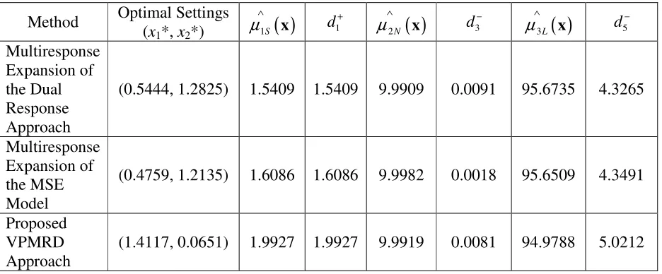
evaluation of the mean and variance at their optimal settings. In terms of the variance, Table 9

shows the optimum operating conditions for each approach, which also represents the deviation

from the target, given that the desired target value is zero. The only result that indicates the goal

of zero variance was achieved is for the response of filtration purity using the proposed VPMRD

approach; all other results slightly exceed zero. Yet, it is important to note that the proposed

method also resulted in the lowest variance for the response of filtration time in comparison to

the other approaches. In terms of the mean, Table 10 shows the evaluation of the mean at the

optimization method considered here. For filtration time, all optimization methods over-achieve

the target, with the multiresponse expansion of the dual response concept producing the

minimum deviation. In terms of filtration volume and purity, all approaches under-achieve the

target. Here, the multiresponse expansion of the MSE and the dual response concepts produce

the minimum deviation for the filtration volume and purity, respectively.

[Table 9 – Approximately Here]

[Table 10 – Approximately Here]

As has been shown with other RD models in the past, we see here that a trade-off exists

between minimizing the variance and minimizing the process bias. Based on the results of this

comparison study, it can be concluded that the proposed model achieves its primary goal of first

minimizing the variance and then attempting to achieve the mean equal to the desired target

value. This logic explains why this method tended to produce the minimum variance, but not the

minimum process bias. Yet, this approach provides a flexible and structured method for

modeling multiresponse RD problems in the presence of responses with differing objectives.

Therefore, this method is useful in situations where minimizing the variance is more critical than

achieving a specific target value for problems involving multiple objectives.

Conclusion

In this work, a new RD optimization approach and framework was proposed, called VPMRD, to

handle situations in which we wish to determine the optimum operating conditions for a system

when the problem entails multiple responses and in cases where it is critically important that the

variance of the responses being considered is minimized. Here, the proposed method utilized

using deviation variables. The objective of the proposed model addressed the inherent goal of

RD where the first priority was to minimize the variance. The proposed optimization approach

was described in detail and illustrated though the use of a numerical example. The results

obtained from this approach were then compared to that of expanded approaches of the

traditional RD optimization models in order to address multiple quality characteristics.

The result of this work provides a method for using RD in real-world situations where

optimal solutions are desired in the face of multiple responses. The approach discussed here

illustrates that there are trade-offs in design between minimizing the variance and achieving the

desired target value. Yet, the specific model proposed here addresses these trade-offs by

References

Cho BR, Park C. Robust design modeling and optimization with unbalanced data. Computers and Industrial Engineering 2005;48(2): 173-80.

Hillier FS, Lieberman GJ. Introduction to operations research. New York: McGraw-Hill, 2001. Kim YJ, Cho BR. Development of priority-based robust design. Quality Engineering 2002;14(3):

355-63.

Kovach J, Cho BR. A D-optimal design approach to robust design under constraints: a new design for six sigma tool. International Journal of Six Sigma and Competitive Advantage 2006;2(4): 389-403.

Lee SB, Park C, Cho BR. Development of a highly efficient and resistant robust design. International Journal of Production Research 2007;45(1): 157-67.

Lin DKJ, Tu W. Dual response surface optimization. Journal of Quality Technology 1995;27(1): 34-9.

Myers RH, Carter WH. Response surface techniques for dual response systems. Technometrics 1973;15(2): 301-17.

Nair VN, Shoemaker AC, The role of experimentation in quality engineering: a review of Taguchi’s contributions. In: Ghosh, S (Ed.). Statistical design and analysis of industrial experiments. New York: Marcel Dekker, 1990. p. 247–77.

Park C, Cho BR. Development of robust design under contaminated and non-normal data. Quality Engineering 2003;15(3): 463-69.

Shin S, Cho BR. Bias-specified robust design optimization and its analytical solutions. Computers and Industrial Engineering 2005;48(1): 129-40.

Taguchi G. Introduction to quality engineering: designing quality into products and processes. New York: Krauss International Publications, 1986.

Taguchi G. System of experimental design: engineering methods to optimize quality and minimize costs. Dearborn, MI: American Supplier Institute, 1987.

Tang LC, Xu K. A unified approach for dual response surface optimization. Journal of Quality Technology 2002;34(4): 437-47.

Figures and Tables

! !

"

# $ %

$ &

# $ &

#

Table 1 General Model of the Proposed VPRMD Framework

Given Design factors: x , i_i =1 2, ,…, n

Responses: y_kt, where

1 2 ,

k= , , , a, , b, c

t = type of quality characteristic (S-, N-, or L-) Fitted response models: Mean: µ_kt

_{( )}

∧

x and variance: 2

_{( )}

σ

∧

x

Desired target values: Mean:

k t

µ

τ ∧ and variance:

2

k t

σ

τ ∧

Find _{Robust design factor specifications:} * _{1 2} i

x , i= , ,…, n

Deviation variables associated with constraints: d , d , gg g 1 2, , , r

− +

=

Satisfy Constraints:

1. System requirements 2. System goals

Minimize Z=_f d , d₁

₍

₎

₍

₎

₍

₎

Table 2 Experimental Design and Observations of Filtration Time for the Multiresponse Chemical Filtration Study

Temperature Pressure Filtration Time (seconds) Coded Units 3 Replications

Average Variance

Treatment No. x1 x2 y1 1S y1 2S y1 3S y1S

2

1S

s

1 -1 -1 3.86 4.03 3.92 3.94 0.007

2 1 -1 3.12 3.07 3.02 3.07 0.003

3 -1 1 2.82 2.79 2.87 2.83 0.002

4 1 1 1.07 0.97 0.99 1.01 0.003

5 -1.414 0 1.30 1.26 1.32 1.29 0.001 6 1.414 0 2.07 2.14 2.11 2.11 0.001 7 0 -1.414 0.60 0.63 0.68 0.64 0.002 8 0 1.414 2.03 2.08 2.04 2.05 0.001

9 0 0 2.12 1.79 2.16 2.02 0.041

10 0 0 2.80 2.52 2.42 2.58 0.039

11 0 0 2.19 2.02 2.14 2.12 0.008

Table 3 Experimental Design and Observations of Filtration Volume for the Multiresponse Chemical Filtration Study

Temperature Pressure Filtration Volume (mL)

Coded Units 3 Replications Average Variance Treatment No. x1 x2 y2 1N y2N2 y2N3 y2N

2

2N

s

1 -1 -1 9.70 9.79 9.73 9.74 0.002

2 1 -1 9.96 9.95 9.93 9.95 0.000

3 -1 1 9.94 9.96 9.97 9.96 0.000

4 1 1 10.00 9.97 9.89 9.95 0.003

5 -1.414 0 9.78 9.87 10.01 9.89 0.013 6 1.414 0 10.02 10.15 9.92 10.03 0.013 7 0 -1.414 9.80 10.04 9.98 9.94 0.016 8 0 1.414 10.10 9.99 10.01 10.03 0.003 9 0 0 10.12 10.01 9.86 10.00 0.001

10 0 0 10.10 9.97 9.85 9.97 0.001

11 0 0 10.08 9.99 10.13 10.07 0.017

12 0 0 9.98 10.11 9.78 9.96 0.004

Table 4 Experimental Design and Observations of Filtration Purity for the Multiresponse Chemical Filtration Study

Temperature Pressure Filtration Purity (%)

Coded Units 3 Replications Average Variance Treatment No. x1 x2 y3 1L y3 2L y3 3L y3L

2

3L

s

Table 5 Proposed VPMRD Optimization Model for the Multiresponse Chemical Filtration Study

Given Design factors, x:

1

x = Temperature (ºF)

2

x = Pressure (psi)

Responses, y:

1S

y = Filtration time (seconds)

2N

y = Filtration volume (mL)

3L

y = Filtration purity (%) Fitted response models:

Mean: µ_{k t}

_{( )}

∧

x from Equations (11), (13), and (15)

Variance: σ_{k t}2

_{( )}

∧

x from Equations (12), (14), and (16) Desired target values: Mean:

k t

µ

τ ∧ and variance:

2 k t σ τ ∧ Mean: 1 0 S µ

τ ∧ =

2 10

N

µ

τ ∧ =

3 100

L

µ

τ ∧ =

Variance: 2 1 0 S σ

τ ∧ =

2 2

0

N

σ

τ ∧ =

2 3

0

L

σ

τ ∧ =

Find _{Robust design factor specifications:} * _{1 2} i

x , i= ,

Deviation variables associated with goals: d , d , g_g− _g+ =1 2, , ,6 Satisfy Constraints:

1. µ_1S

_{( )}

∧

≤

x 2. 9 5. µ_2N

_{( )}

∧

≤ x ≤ 3. µ_3L

_{( )}

∧

≥ x

Goals:

1. µ1S

( )

∧

− +

+ − =

x 4. σ22N

( )

∧

− +

+ − =

x

2. σ2_1S

_{( )}

∧

− +

+ − =

x 5. µ_3L

_{( )}

∧

− +

+ − =

x

3. µ_2N

_{( )}

∧

− +

+ − =

x 6. 2

_{( )}

3L d6 d6 0

σ ∧ − + + − = x Bounds:

1. Design factors: 1 414− . ≤x_i ≤1 414 for . i=1 2,

2. Deviation variables: d , dg g 0

− +

≥ and dg dg 0

− +

⋅ = for g=1 2, , ,6

Minimize

_{( )}

_{( )}

_{( )}

_{( )}

_{( )}

_{( )}

₍

₎

_{( )}

_{( )}

3 3 3

2 4 6 1 3 3 5

Z M d+ M d+ M d+ d+ d− d+ d− 

Table 6 Results of the Proposed VPMRD Approach for the Multiresponse Chemical Filtration Study

Optimal Settings x* = (1.4117, 0.0651)

Mean

( )

1S

µ

∧

x = 1.9927

( )

µ

∧

x = 9.9919

( )

3L

µ

∧

x = 94.9788

Variance

( )

x = 0.0017

( )

2 2N

σ

∧

x = 0.0081

( )

2 3L

σ

∧

x = 0

Table 7 Results of the Multiresponse Expansion of the Dual Response Approach for the Multiresponse Chemical Filtration Study

Optimal Settings x* = (0.5444, 1.2825)

Mean

( )

1S

µ

∧

x = 1.5409

( )

2N

µ

∧

x = 9.9909

( )

3L

µ

∧

x = 95.6735

Variance

( )

x = 0.0033

( )

2 2N

σ

∧

x = 0.0033

( )

2 3L

σ

∧

Table 8 Results of the Multiresponse Expansion of the MSE Model for the Multiresponse Chemical Filtration Study

Optimal Settings x* = (0.4759, 1.2135)

Mean

( )

1S

µ

∧

x = 1.6086

( )

µ

∧

x = 9.9982

( )

3L

µ

∧

x = 95.6509

Variance

( )

x = 0.0069

( )

2 2N

σ

∧

x = 0.0033

( )

2 3L

σ

∧

x = 0.0311

Table 9 Comparison of Optimization Methods in Determining the Optimal Design Factor Settings and the Evaluation of the Variance

for the Multiresponse Chemical Filtration Study

Method Optimal Settings

(x1*, x2*)

( )

2 1S

σ

∧

x 2

_{( )}

σ

∧

x 2

_{( )}

σ

∧

x

Multiresponse Expansion of the Dual Response Approach

(0.5444, 1.2825) 0.0033 0.0033 0.0088

Multiresponse Expansion of the MSE Model

(0.4759, 1.2135) 0.0069 0.0033 0.0311

Proposed VPMRD

Table 10 Comparison of Optimization Methods in Determining the Optimal Design Factor Settings and the Evaluation of the Mean

for the Multiresponse Chemical Filtration Study

Method Optimal Settings

(x1*, x2*) µ1S

( )

∧

x d1

+

( )

2N

µ

∧

x d3

−

( )

3L

µ

∧

x d5

−

Multiresponse Expansion of the Dual Response Approach

(0.5444, 1.2825) 1.5409 1.5409 9.9909 0.0091 95.6735 4.3265

Multiresponse Expansion of the MSE Model

(0.4759, 1.2135) 1.6086 1.6086 9.9982 0.0018 95.6509 4.3491

Proposed VPMRD Approach

(1.4117, 0.0651) 1.9927 1.9927 9.9919 0.0081 94.9788 5.0212