Control of Lagrange point orbits using solar sail propulsion

CONTROL OF LAGRANGE POINT ORBITS USING SOLAR SAIL PROPULSION

John Bookless*, Colin McInnes+

[email protected]

*Dept. of Aerospace Engineering, University of Glasgow, Glasgow G12 8QQ, Scotland, UK +

Dept. of Mechanical Engineering, University of Strathclyde, Glasgow G1 1XJ, Scotland, UK

Abstract

Several missions have utilised halo orbits around the L1 and L2 Lagrange points of the Earth-Sun system. Due to the instability of these orbits, station-keeping techniques are required to prevent escape after orbit insertion. This paper considers using solar sail propulsion to provide station-keeping at quasi-periodic orbits around L1and L2. Stable manifolds will be identified which provide near-Earth insertion to a quasi- periodic trajectory around the libration point. The possible control techniques investigated include solar sail area variation and solar sail pitch and yaw angle variation. Hill’s equations are used to model the dynamics of the problem and optimal control laws are developed to minimise the control requirements. The constant thrust available using solar sails can be used to generate artificial libration points sunwards of L1 or Earthwards of L2. A possible mission to position a science payload sunward of L1 will be investigated. After insertion to a halo orbit at L1, gradual solar sail deployment can be performed to spiral sunwards along the Sun-Earth axis. Insertion ΔV requirements and area variation control requirements will be examined. This mission could provide advance warning of Earthbound CME (Coronal Mass Ejections) responsible for magnetic storms.

Introduction

Solar sailing is an emerging form of propulsion which utilises solar radiation pressure to provide a useful thrust. The sail is a thin reflective film with a thickness of order 2 μm, with a large reflective area in order to intercept a flux of photons. A key advantage of solar sails over conventional propulsion systems is that missions are not constrained by the ΔV available from stored reaction mass. This enables many new and exciting high-energy mission concepts. Several authors including Leipold1,2, Macdonald3 and Hughes4 have recently investigated the potential of solar sails for planetary missions.

McInnes5-7, Farquhar8, Forward9 and Morrow10 have demonstrated that the constant acceleration from a solar sail can be used to generate artificial libration points in the Earth- Sun three-body problem. This is achieved by directing the thrust due to solar radiation pressure in the anti-Sun direction adding to the centripetal force in the rotating Earth-Sun frame. A continuum of libration points can be produced Earthwards of L2 or sunwards of L1.

Halo orbits can be generated around these libration points by selecting suitable initial

conditions which lead to periodic solutions of the linearised three-body equations. Due to the instability of these orbits, station-keeping techniques must be applied to prevent escape after orbit insertion. The solar sail can be made to track the nominal trajectory by applying trims to the sail reflective area or sail pitch angle.11 Optimal control laws are applied to minimise the variation of sail area or pitch angle required to provide orbit control.

The Geostorm mission, developed at JPL, aims to position a science payload Sunwards of L1. After insertion to a halo orbit around L1, the solar sail is slowly deployed resulting in a spiraling motion Sunwards along the Sun-Earth line. This would enable continuous monitoring of the solar wind to detect CMEs. The increase in charge density of the solar wind can result in magnetic storms being experienced in the vicinity of the Earth. This space weather phenomenon poses a considerable risk to geostationary satellites which can be bombarded by high energy, charged particles.12

Solar sails consist of large area gossamer structures with a reflective coating which intercept the solar photon flux. Photons incident on the sail impart momentum and the reflection results in a reaction force, thus providing double the force which would be imparted to an absorbing surface. Possible sail substrate candidates include the plastics Mylar, Kapton or CP-1 polyimide film developed at NASA-Langley. 13

The solar sail acceleration is dependent on the areal density, also known as the sail loading. The sail acceleration, κ, is defined by

n φ α βμ

η ₂ cos2 cos2

s

R

s

= (1)

where η the sail reflectivity, Rs is the distance from the Sun, α is the pitch angle of the sail normal vector n to the Sun-line, φ is the yaw angle of the sail normal vector to the Sun-line and β is the solar sail lightness parameter defined as the ratio of solar radiation pressure to gravitational attraction

σ μ π β

s c

s L 2

= (2)

where solar luminosity Ls = 3.86x10 26

W, c is the speed of light, μs is the solar gravitational parameter and σ is the ratio of solar sail mass to surface area known as the loading parameter. Decreasing sail loading increases the lightness number thus increasing the characteristic acceleration.14

Hill’s Equations

Hill’s approximation of the circular restricted three-body problem can be adapted to include the dynamical effects of solar radiation pressure as

x

x x

y

x−2Ω =− +3Ω2 +κ 3

r & &

& (3.1)

y

y x

y+2Ω =− ₃+κ

r & &

& (3.2)

z

z z

z=− −Ω2 +κ 3

r &

& (3.3)

where r= x2+y2+z2 is the separation between the solar sail and the Earth, Ω is the angular velocity of the Earth orbiting the Sun and the acceleration due to solar radiation

pressure =κxi+κyj+κzk. These equations

are non-dimensionalised using 1RE (Earth Radii) as the characteristic length and

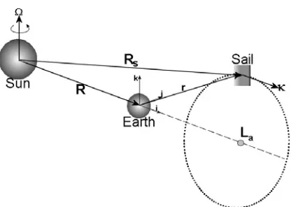
characteristic time τ = L3 μE , where μE is the Earth gravitational parameter.15 A schematic of the three-body model is provided in Fig 1.

[image:2.612.329.537.231.379.2]

It is assumed that the Earth is located at the origin and the separation distance between the Sun and Earth, R, is constant. The sail is assumed to have negligible mass relative to the larger bodies.

Fig 1: Schematic of Sun-Earth Model with artificial libration point La

Jacobi Integral

The Jacobi integral can be extracted from Hill’s equations with the form

C z

x +Ω − =

Ω −

− r

r

v2 2 3 2 2 2 2 2 .

(4)

where _{v= x&}2_+y&2_+z&2 _{is the velocity}

magnitude and r=xi+yj+zk.

The constant of integration, C, is analogous to

the total orbit energy E, where . The

Jacobi constant can be evaluated for a set of initial conditions. The obtained value of C can be used to generate a surface of zero velocity. This surface of constant energy, also referred to as Hill’s surface, bounds the orbital motion as it is forbidden for the trajectory to intersect the surface.

E C=2

The L1 and L2 Lagrange points of Hill’s problem are symmetric about the origin on the x-axis. The position can be calculated from Eqn (3) by setting the acceleration and velocity components . Solving Eqn (3.1) for x,

gives the Lagrange point location

0 = = = = =

=x y y z z

x& && & && & &&

( )

₂ 13

3Ω −

± =

x .

Substituting into Eqn (4), the Jacobi constant evaluated at the Lagrange points has the form

( )

23 9Ω − =

C for the ballistic case, κ=0.15

An artificial libration point, located at xo, can be generated using the solar sail acceleration to cancel part of the gravitational forces exerted by the Earth and the Sun. The required acceleration is given by

o o o o x r x 2

3 −3Ω =

κ (5)

[image:3.612.326.539.74.288.2]

where κ=κ_oi in the case of a Sun-pointing sail.

Table 1 provides the values of Jacobi Constant for the contours shown in Fig 2. These contours represent constant energy surfaces of zero-velocity. The values of C, evaluated at the libration points represent a critical value for a closed surface. As orbit energy is increased, a gap opens in the surface around the libration point.

No. xo

RE

Jacobi Constant C

Acceleration

κ

1 234.46 -0.012795 0

2 210 -0.015626 6.383x10-6

3 190 -0.0182518 1.296 x10-5

4 170 -0.021287 2.141 x10-5

[image:3.612.67.294.423.680.2]

5 150 -0.024921 3.281 x10-5

Table 1: Jacobi Constant for libration points

Fig 2: Hill’s Surfaces for onaxis libration points Quasi-periodic Orbit Solution

Hill’s equations are linearised about the libration point, new coordinates ξ=x−x_o, η=y− y_o and

o

z z− =

ζ , where (xo, yo, zo). The linearised

equation can be represented by the state equation x& =Ax, where the state vector

[

]

Τ

= ξ η ς ξ& η& ς&

x , The linear coefficient

matrix is defined as

(6) ⎥ ⎥ ⎥ ⎥ ⎥ ⎥ ⎥ ⎥ ⎦ ⎤ ⎢ ⎢ ⎢ ⎢ ⎢ ⎢ ⎢ ⎢ ⎣ ⎡ Ω − Ω = 0 0 0 0 0 0 0 2 0 0 0 2 0 0 0 1 0 0 0 0 0 0 1 0 0 0 0 0 0 1 0 0 0 zz yy xx f f f A

where fxx, fyyand fzz are the 2 nd

order derivatives of the pseudo-potential

x z x z y x

f = +Ω (3 − )+κ

2 1 ) , ,

( 2 2

2

r (7)

The partial derivatives are evaluated at the libration point.

In the x-y plane the linear solution produces two real eigenvalues and two imaginary eigenvalues. Using the method outlined by Szebehely16, the terms containing real eigenvalues are suppressed which obtains the oscillatory solution

( )

λ τ

ξ= Ayvsin xy (8.1)

( )

λ τ

η= Aycos xy (8.2)

( )

λ τ

ς = Aycos zy (8.3)

where Ay is the y-axis orbit amplitude.

The in-plane eigenvalue λ_xy is defined as

(

) (

)

(

)

_⎟⎟ ⎠ ⎞ ⎜ ⎜ ⎝ ⎛ − − − Ω − + + Ω −

= xx yy xx yy xx yy

xy 4 f f 4 f f 4 f f

2

1 _{2 2} 2

λ

(9)

and the out of plane eigenvalue λ_z = f_zz . The eigenvector relating the x and y coordinates is expressed as v=−

(

λ_xy2 +3Ω2

)

2Ωλ_xy.

non-rational the orbit is quasi-periodic producing a Lissajous trajectory about the libration point.

Evaluating the linear solution at time τ=0 yields the initial conditions xo =0, yo =Ay, zo =0,

v A

x&o = yλxy , y&o =0 and z&o = Ayλz. 17

These

conditions will be used to identify stable manifolds which wind onto the nominal Lissajous trajectory.

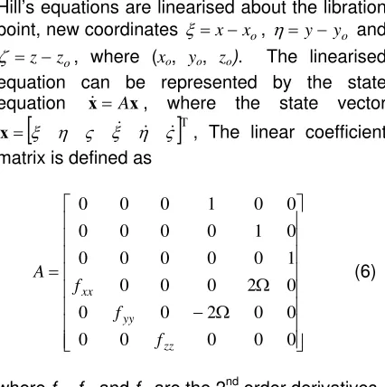
Fig 3: Quasi-periodic Trajectory produced by linear solution to Hill’s Equations

Optimal Controller

Optimal control laws can be applied to help select gains which use sail area or pitch angle control for station-keeping. The control problem can be modeled using the state equations

(10.1) ) ( ) ( )

(t Axt Bu t

x& = +

(10.2)

) ( ) (t Cxt

y =

where A is the linear coefficient matrix defined in Eq (6), B is the control matrix, C is the output matrix, u(t) is the control vector, x(t) is the state vector and y(t) is the output vector.

The acceleration components can be derived from Eq (1) as

(11.1)

φ α κ

κ 3 3

cos cos ) (t x= φ φ α κ

κy = (t)cos3 cos2 sin (11.2)

α φ α κ

κz = (t)cos2 cos2 sin (11.3)

The continuous variation of the distance between the Sun and the solar sail is modeled

using κ(t)=κ_o

(

R_s R(t)

)

2 where Rs is the separation distance between the Sun and solar sail at the nominal orbit and R(t) is the separation distance at time t.

The solar sail area varies linearly with the acceleration. The area control matrix is constructed using the partial derivatives

φ α κ

κ _cos3 _cos3

) ( =

∂ ∂

t

x _(12.1)

φ φ α κ κ sin cos cos ) ( 2 3 = ∂ ∂ t y (12.2) α φ α κ κ sin cos cos ) ( 2 2 = ∂ ∂ t

z _(12.3)

such that Τ ⎥ ⎦ ⎤ ⎢ ⎣ ⎡ ∂ ∂ ∂ ∂ ∂ ∂ = ) ( ) ( ) ( 0 0 0 t t t

B x y z

κ κ κ κ κ κ (13)

At the nominal orbit, the pitch and yaw angles

0

= =φ

α . The resulting control matrix has the form B=

[

0 0 0 1 0 0

]

Τ and the output matrix C is a 6x6 identity matrix I6x6.

For a pitch and yaw angle controller, the control matrix has the form

Τ ⎥ ⎥ ⎥ ⎥ ⎦ ⎤ ⎢ ⎢ ⎢ ⎢ ⎣ ⎡ ∂ ∂ ∂ ∂ ∂ ∂ ∂ ∂ ∂ ∂ ∂ ∂ = φ κ φ κ φ κ α κ α κ α κ z y x z y x B 0 0 0 0 0 0 (14)

The partial derivatives can be expressed as

φ α α κ

α

κ 2 3

cos sin cos ) ( 3 t

x ₌₋

∂ ∂ (15.1) φ φ α α κ α κ sin cos sin cos ) (

3 t 2 2

y ₌₋

∂ ∂ (15.2)

(

α φ α κ α

)

κ 3 2 2

tan 2 1 cos cos ) ( − = ∂ ∂ t

z _(15.3)

φ φ α κ φ κ sin cos cos ) (

3 t 3 2 x ₌₋

∂ ∂ (15.4)

(

φ α φ κ φ

κ _{3 3 2}

tan 2 1 cos cos ) ( − = ∂ ∂ t y

)

(15.5) φ φ α α κ φ κ sin cos sin cos ) ( 2 t 2

z ₌₋

∂ ∂

[image:4.612.85.270.191.381.2]

Evaluating at the nominal orbit conditions with acceleration κ(0)≡κ_o and pitch and yaw angle

0

= =φ

α , results in a control matrix of the form

(16) Τ ⎥ ⎦ ⎤ ⎢ ⎣ ⎡ = 0 0 0 0 0 0 0 0 0 0 o o B κ κ

Optimal control theory provides a method for selecting a gain matrix which suppresses any unstable eigenvalues based on a cost function V

(17)

[

∫

∞ + = t d N Q

V x'(τ) x(τ) u'(τ) u(τ)

]

τ

where t is the initial integration time, Q is the state-weighting matrix and N is the control-weighting matrix. The 1st term inside the brackets represents the penalty on the deviation of state vector x from the nominal orbit conditions and the 2nd term represents the cost of control which limits the size of the control signal. The aim is to select a gain matrix G that minimises the performance function V. This can be achieved using the Ricatti Equation

(18) Q M B MBN M A MA

M = + − +

− & ' −1 '

where M is the performance matrix and is related to the performance function such that

.

Mx x

V = ' Provided that M converges to a limit

as , it can be assumed that .

Equation (18) can be solved for M which enables the optimal gain matrix to be calculated

using .

∞ →

t M& →0

M B N

G= −1 ' 18

In the case of area control, the gain matrix contains 6 elements. These are multiplied by the difference between the desired and actual position and velocity to obtain the required x-axis velocity variation as

ς δ η δ ξ δ δς δη δξ

δκx=G₁ +G₂ +G₃ +G₄ &+G₅ &+G₆ &

(19)

The desired position is determined using the solution to the linear Hill’s problem provided in Eq (8). The actual position and velocity relative to the libration point are denoted by

(

ξ,η,ς,ξ&,η&,ς&

)

.

The variation of position and velocity is determined using

δξ=ξ −A_yνsin

( )

λ_xyτ (20.1) δη=η−Aycos

( )

λxyτ (20.2)

δς =ς−Aysin

( )

λzτ (20.3)

δξ&=ξ&−A_yvλ_xycos

( )

λ_xyτ (20.4) δη&=η&+Ayλxysin

( )

λxyτ (20.5) δς&=ς&−Ayλzcos

( )

λzτ (20.6)

In the case of pitch and yaw angle control, the gain matrix, G, yields 6x2 elements. The pitch angle variation is determined using

ς δ η δ ξ δ δς δη δξ

δα=G₁₁ +G₁₂ +G₁₃ +G₁₄ &+G₁₅ &+G₁₆ &

(21.1)

and the yaw angle variation as

ς δ η δ ξ δ δς δη δξ

δφ=G₂₁ +G₂₂ +G₂₃ +G₂₄ &+G₂₅ &+G₂₆ &

(21.2)

These angles can be substituted into Eq (11) to calculate the resulting Cartesian acceleration components. Both these control techniques will be demonstrated for Lissajous trajectories around the Lagrange points.

Insertion to Lissajous orbit around L2

It is impossible to direct the solar sail normal acceleration sunward. Therefore, to enable the controller to prevent escape in the anti-Sun direction, the Lissajous trajectory will orbit a libration point slightly sunward of L2, at xo=230RE with selected radius Ay=20RE. An insertion trajectory which winds onto this orbit is provided in Fig 4, bound within a Hill’s surface with Jacobi constant C= -0.0131.

The closest approach distance to the Earth is 19.1RE. This trajectory was identified by numerically integrating the Lissajous orbit initial conditions and selecting the closest approach distance to the Earth.

Using the mirror image transform

(

)

(

x y z x y z t

)

t z y x z y x − − − −

→ & & & &

& &

the closest approach conditions can be transformed into a new set of initial conditions which wind onto the nominal Lissajous orbit. The nominal acceleration for this orbit

κo=0.00831mms -2

.

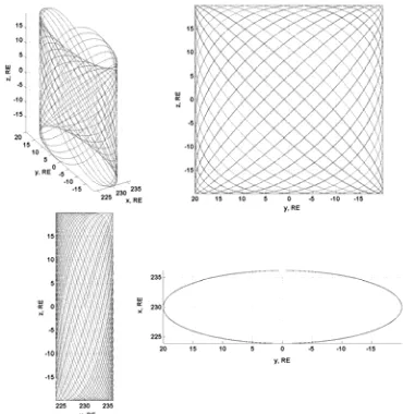
Figure 5 demonstrates the insertion to the stable manifold from a 200 km altitude Earth orbit, inclined 7.3o relative to the ecliptic plane. A Hohmann transfer manoeuvre is performed with an initial kick-stage ΔV=2.94kms-1. The second kick-stage, ΔV=1.831kms-1 is directed 11.5o Sunwards relative to the y-z plane. The solar sail is deployed immediately after this second kick-stage arriving at the nominal orbit after 91 days.

Fig 4: Insertion manifold for Lissajous orbit around L2

Fig 5: Insertion requirements from a 200km

altitude Earth orbit

Area variation Control at L2

The controller is activated when the solar sail arrives at the nominal orbit. Figure 6a shows the solar sail controlled in a Lissajous orbit at L2 for a duration of 15 years. A close-up section of the Lissajous orbit is provided in Fig 6b.

Figure 7 shows the required acceleration and area variation for a 200kg payload + sail mass. The acceleration varies between 0.00682mms-2 and 0.0114mms-2,which corresponds to an area variation between 152m2 and 254m2. Sail area variation can be achevied using 4 small, controllable vanes attached to the central payload. For sail loading σ=12gm-2, the total required sail mass is 3kg allowing a payload mass of 197kg. The station-keeping requirements correspond to an annual ΔV of approximately 280ms-1.

[image:6.612.95.273.277.444.2]

The gradient of sail area against payload mass is 1.2917 for sail loading σ=12gm-2. This enables the sail area required for orbit control to be determined for a desired payload mass. In the case of a small payload with mass 100kg, station-keeping could be achieved using a 129m2 sail. A larger payload with mass 2000kg would require a 2583m2 solar sail.

[image:6.612.329.538.412.511.2]

Fig 6a: Insertion to area variation controlled Lissajous trajectory around L2

[image:6.612.75.289.492.601.2] [image:6.612.381.487.549.684.2]

Fig 7: Acceleration and area variation required to control orbit

Gains: G1=4.839x10

-7

G2=-8.630x10 -8

G3=1.485x10 -15

G4=8.295x10 -4

G

5

=

4.394x10-4

G

6

=

-4.048x10-12

Angle variation Control at L2

Using the same stable manifold for insertion, pitch and yaw angle control can be performed at the nominal orbit to provide station-keeping. The controller is activated as the solar sail approaches the nominal orbit and the sail is fully deployed to provide constant acceleration of

0.01mms-2. This acceleration increase

corresponds to 1.2κo and is necessary to prevent Earthwards escape from the nominal orbit after insertion.

[image:7.612.334.538.73.188.2]

Figure 8a demonstrates the orbit insertion of a solar sail to a Lissajous trajectory controlled for an duration of 15 years. Figure 8b shows an enlarged view of the Lissajous orbit.

Fig 9 shows the pitch and yaw angle variation required to control this orbit. The pitch angle varies between -42.9o and 2.9o. The yaw angle varies between -0.69o and 0.78o.

[image:7.612.75.286.77.240.2]

A total sail and payload mass of 200kg could be controlled with a 222m2 sail using this method. This is around 30m2 less than the total sail area required using area variation control for the same mass. The payload mass-area gradient is 1.1268 for sail loading σ=12gm-2. A small 100kg payload could be controlled using a 113m2 sail or a large 2000kg payload would require a 2254m2 sail.

[image:7.612.355.516.233.371.2]

Fig 8a: Insertion to angle variation controlled Lissajous trajectory around L2

Fig 8b: Close-up of angle variation controlled Lissajous orbit

Fig 9: Pitch and Yaw angle variation required to control Lissajous orbit

Gain φ:

G1=-5.157x10-14G2=9.628x10-15G3=1.568x10-6 G4=-8.788x10-11

G

5

=

-4.631x10-11

G

6

=

1.7564

Gain α:

G1=0.9103 G2=-0.1618 G3=4.032x10 -14

[image:7.612.327.534.419.577.2]

Insertion to Lissajous orbit around L1

Artificial libration points can be generated Sunwards of L1. A nominal Lissajous orbit will be generated around a libration point at xo=-240RE with radius 20RE. This requires a nominal acceleration κo=0.0141mms

-1 .

[image:8.612.95.271.353.508.2]

A stable manifold was identified which passes within 1.15 RE of the Earth. After insertion, the solar sail winds onto the desired orbit. Figure 10 shows this trajectory bound within a Hill’s surface with Jacobi constant C=-0.0120. As the solar sail travels sunwards, the radiation pressure exerts a drag force. Due to this drag, increased energy is required to generate a gap in the zero-velocity surface at the libration point.

[image:8.612.93.268.356.688.2]

Figure 11 demonstrates the insertion to the stable manifold using a Hohmann transfer manoeuvre from a 200km altitude parking orbit. The solar sail is deployed immediately after the 2nd kick-stage and winds onto the nominal orbit within 320 days.

Fig 10: Insertion manifold for Lissajous orbit around L1

Fig 11: Insertion requirements from a 200km

altitude Earth orbit

Area variation control at L1

As before, the controller is activated when the solar sail arrives at the nominal orbit. Figure 12a shows a Lissajous orbit controlled around the artificial libration point for 15 years. An enlarged view of the Lissajous orbit is provided in Fig 12b.

Figure 13 shows the acceleration and area variation required to control the orbit. The acceleration varies between 0.0115mms-2 and 0.0159mms-2. For a 200kg sail and payload mass, this corresponds to an area variation between 246m2 and 340m2. A sail loading of

σ=12gm-2 would require a sail of 4kg enabling control of a 196kg payload at this libration point. The station-keeping requirement corresponds to an annual ΔV of approximately 395ms-1.

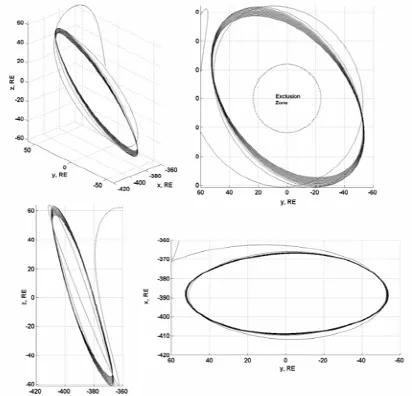
[image:8.612.330.537.405.496.2]

There is a telemetry exclusion zone sunwards of the Earth as the solar radio disk interferes with spacecraft communication. At the libration point this corresponds to a 93,500km radius disk in the y-z plane.19 During the control period, the solar sail spends approximately 1/4th of the time within the exclusion region.

[image:8.612.92.269.528.687.2]

Fig 12a: Insertion to area variation controlled Lissajous trajectory around L1

[image:8.612.359.510.539.681.2]

[image:9.612.349.517.72.209.2]

Fig 13: Area and acceleration variation required to control orbit at L1

Gains:

G1 =4.655x10-7 G2 =-8.379x10-8 G3 =1.4x10-16 G 4 =8.068x10-4 G₅ = 4.355x10-4 G₆ = 2.345x10-12

Angle variation Control at L1

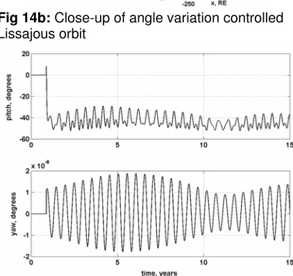
[image:9.612.73.285.72.242.2]

Pitch and yaw angle variation can also be applied to control the Lissajous trajectory at L1. Figure 14a shows the orbit controlled using pitch and yaw angle variation. The sail is fully deployed when it reaches the nominal orbit producing an acceleration of 0.0247mms-2. An enlarged view of the trajectory is provided in Fig 14b.

The pitch and yaw angle variation is shown in Fig 15. The pitch angle varies between -52.3o and 8.3o. The yaw angle varies between -1.78x10-6 o and 1.89x10-6 o.

[image:9.612.326.537.209.408.2]

During the control period, the solar sail spends approximately 1/5th of the time within the exclusion region.

Fig 14a Insertion to angle variation controlled Lissajous trajectory around L1

Fig 14b: Close-up of angle variation controlled Lissajous orbit

Fig 15: Pitch and yaw angle variation required to control orbit at L1

Gain φ: G1=1.872x10

-13

G2=-3.405x10 -14

G3=1.283x10 -17

G4=-3.295x10 -10

G

5

=

1.836x10-10

G

6

=

3.19x10-6

Gain α:

G1=0.916 G2=-0.0575 G3=-5.666x10-14 G4=554.3190

G

5

=

309.7840

G

6

=

1.836x10-10

Geostorm Mission

Currently there are several spacecraft which orbit the L1 point including SOHO20 and ACE21. These spacecraft provide data regarding the solar wind density and velocity.

[image:9.612.86.278.562.662.2]

magnetosphere on the day-side. Lower altitude satellites can also be affected by the expansion of the Earth’s atmosphere leading to increased drag affects. Probes orbiting L1 can provide approximately 30 minutes advance warning of approaching CME.

It has been demonstrated that a solar sail can be used to provide station-keeping at an orbit Sunward of L1. The Geostorm mission, developed at JPL, aims to position a science payload sunwards of L1 providing increased warning time of local changes in solar wind density.12

An un-deployed solar sail can be transported to a Lissajous orbit around L1. The sail can then be slowly deployed, spiralling sunwards along the Sun-line to a new libration point orbit further from the Earth.

A ballistic (κ=0) manifold was idenitifed which winds onto a Lissajous orbit of radius 50RE. The manifold passes within 11.15RE of the Earth. Figure 16 shows the insertion trajectory bound within a zero-velocity surface with Jacobi constant C=-0.01226.

A Hohmann transfer manoeuvre which inserts the solar sail onto the stable manifold from a 200km altitude orbit is shown in Figure 17. After the second kick-stage, the solar sail winds onto the Lissajous orbit within 186.5 days.

[image:10.612.340.526.73.243.2]

Fig 16: Insertion trajectory for Geostorm Mission

Fig 17: Insertion requirements from a 200km altitude Earth orbit

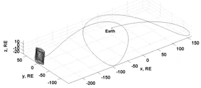
Figure 18a shows the complete trajectory including ballistic insertion and sail deployment. The sail is slowly deployed over the period of 561 days and arrives at a halo orbit around a new libration point 390RE sunward of the Earth. In this case, frequency control is applied using the area controller to match the in-plane and out-of-plane frequencies.22

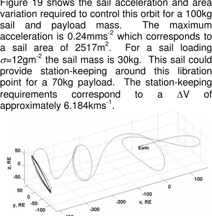
[image:10.612.324.540.471.691.2]

An enlarged view of the final halo orbit is provided in Fig 18b. At this distance, the exclusion zone to avoid solar interference has a radius of 150,000km. It is clear that the halo orbit remains outside the exclusion zone throughout the 15 year control period.

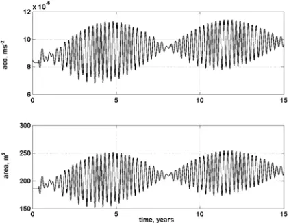
Figure 19 shows the sail acceleration and area variation required to control this orbit for a 100kg sail and payload mass. The maximum acceleration is 0.24mms-2 which corresponds to a sail area of 2517m2. For a sail loading

σ=12gm-2 the sail mass is 30kg. This sail could provide station-keeping around this libration point for a 70kg payload. The station-keeping

requirements correspond to a ΔV of

approximately 6.184kms-1.

Fig 18a: Insertion to Lissajous orbit at L1

[image:10.612.97.270.474.636.2]

[image:11.612.79.285.74.272.2] [image:11.612.75.287.78.455.2]

Fig 18b: Enlarged view of the final halo orbit achieved using area control

Fig 19: Sail acceleration and area variation for Geostorm mission

Conclusions

This paper has demonstrated a possible, near-term application of solar sails for station-keeping in orbits near the Lagrange points of the three-body problem. Relatively small sail area requirements, achievable with present day technology, could provide an attractive alternative to using chemical or solar electric propulsion for libration point missions.

A possible Geostorm mission trajectory was outlined using slow deployment of a solar sail to position a science payload sunward of L1. Initial delivery to an orbit around L1offers the option of a ‘piggy-back’ insertion before sail deployment. The large ΔV requirements of 6kms-1 per year indicate that solar sails are the only feasible propulsion option for this mission.

Acknowledgements

This work was carried out with part financial support from the Lockheed Martin Corporation Advance Technology Centre, Palo Alto, CA.

References

1 _{Leipold, M, et al, ‘Solar Sail Technology for Advanced}

Space Missions’, Acta Astronautica, Vol 39(1-4), 1996, pp143-151

2 _{Leipold, M, ‘To the Sun and Pluto with Solar Sails and}

Micro-Sciencecraft’, Acta Astronautica, Vol 45 (9-5), 1999, pp. 549-555

3_{Hughes, G, et al, ‘Analysis of a Solar Sail Mercury Sample}

Return Mission’, 55th _{International Astronautical Congress, 2004,}

Vancouver, IAC-04-S.2.b.08

4 _{Macdonald, M, McInnes, C.R., ‘A Near-Term Roadmap for}

Solar Sailing’, 55th _{International Astronautical Congress, 2004,}

Vancouver, IAC-04-U.1.09

5 _{McInnes, C.R., McDonald, A.J.C., Simmons, J.F.L. and}

MacDonald, E.W., ‘Solar Sail Parking in Restricted Three Body Systems’, Journal of Guidance, Control and Dynamics, Vol 17, No 2, 1994, pp339-406

6 _{McInnes, C.R., ‘Artificial Lagrange Points for a Non-Perfect}

Solar Sail’, Journal of Guidance, Control and Dynamics, Vol 22, No 1, 1999, pp. 185-187

7 _{McInnes, C.R., ‘Passive Control of Displaced Solar Sail}

Orbits’, Journal of Guidance, Control and Dynamics, Vol. 21, No 6, Nov-Dec, 1998, pp. 975-982

8 _{Farquhar, R, ‘Limit Cycle Analysis of a controlled libration}

point satellite’, The Journal of the Astronautical Sciences, Vol XVII, No. 5, pp 267-291, 1970

9 _{Forward, R.L, ‘Statite: A Spacecraft that does not orbit’,}

Journal of Spacecraft, Vol.28, No. 5, Sept-Oct, 1991, pp 606-611

10 _{Morrow, E, Scheeres, D.J., Lubin, D, ‘Solar sail orbit} operations at asteroids’, Journal of Spacecraft and Rockets, Vol. 38, No 2, Mar-Apr, 2001, pp. 279-286

11 _{Bookless, J, McInnes, C.R, ‘Dynamics and control of}

displaced non-Keplerian orbits using solar sail propulsion’, Journal of Guidance, Control and Dynamics, Vol 29, No3, pp 527-537, 2006

12 _{West, J, Derbes, B, ‘Solar Sail Vehicle System Design for the} Geostorm Warning Mission’, AIAA-2000-5326

13 _{Murphy, D.M., et al, ‘Demonstration of a 10m Solar Sail} System’, 45th _{AIAA Structures, Structural Dynamics & Materials} Conference, AIAA 2004-1576

14 _{McInnes, C.R, ‘Solar Sailing: Technology, Dynamics and} Missions Applications’, Springer-Praxis Series in Space Science and Technology, Springer-Verlag, Berlin, 1999

15 _{Villac, B.F., Scheeres, D.J., ‘Escaping Trajectories in the Hill} Three-Body Problem and Applications’, Journal of Guidance, Control and Dynamics, Vol 26, No 2, Mar-Apr 2003

16 _{Szebehely, V, ‘Theory of Orbits – The restricted problem of} three bodies’, Academic Press Inc., NewYork and London, 1967

17 _{Cielaszyk, D and Wie, B, ‘New Approac to Halo Orbit} Determination and Control’, Journal of Guidance, Control and Dynamics, Vol. 19, No. 2, Mar-Apr, 1996

18 _{Friedland, B, ‘Control System Design: An introduction to} state space methods’, McGraw-Hill Series in Electrical Engineering, 1986, Chap 9, pp 337-369

19 _{Farquhar, R.W., et al, ‘Mission Design for a Halo Orbiter of} the Earth’, J. Spacecraft, Vol 14, No. 3, 1977

20 _{Bouffard, M, et al, ‘SOHO: A Modular Spacecraft Concept to} allow flexible payload integration and efficient development’, Acta Astronautica, Vol. 37, pp 277-291, 1995

21 _{Stone, E.C., et al, ‘The Advance Composition Explorer’,} Space Science Reviews, Vol 86, No 1-4, pp 1-22, 1998