rspa.royalsocietypublishing.org
Research
Cite this article:Payne GS, Pascal R, Vaillant G. 2015 On the concept of sloped motion for free-floating wave energy converters.Proc. R. Soc. A471: 20150238.
http://dx.doi.org/10.1098/rspa.2015.0238
Received: 10 April 2015 Accepted: 20 August 2015
Subject Areas:
ocean engineering, energy, mechanical engineering
Keywords:
wave energy, boundary element method, WAMIT, optimization
Author for correspondence: Grégory S. Payne
e-mail:[email protected]
Electronic supplementary material is available at http://dx.doi.org/10.1098/rspa.2015.0238 or via http://rspa.royalsocietypublishing.org.
On the concept of sloped
motion for free-floating wave
energy converters
Grégory S. Payne
1
, Rémy Pascal
2
and
Guillaume Vaillant
3
1
Institute for Energy Systems, University of Edinburgh,
Edinburgh EH9 3FB, UK
2
Abengoa Seapower, ETTC, Alrick Building, The King’s Buildings,
Edinburgh EH9 3JL, UK
3
Institut Jean Le Rond d’Alembert, Université Pierre et Marie Curie,
Place Jussieu, Paris, France
A free-floating wave energy converter (WEC) concept whose power take-off (PTO) system reacts against water inertia is investigated herein. The main focus is the impact of inclining the PTO direction on the system performance. The study is based on a numerical model whose formulation is first derived in detail. Hydrodynamics coefficients are obtained using the linear boundary element method package WAMIT. Verification of the model is provided prior to its use for a PTO parametric study and a multi-objective optimization based on a multi-linear regression method. It is found that inclining the direction of the PTO at around 50◦ to the vertical is highly beneficial for the WEC performance in that it provides a high capture width ratio over a broad region of the wave period range.
1. Introduction
Wave energy technology has now evolved from early academic research involving scaled model testings and theoretical investigations [1,2] to full-scale devices developed industrially and deployed in the ocean [3–5]. There is, however, no consensus on what type of wave energy converter (WEC) is the most promising and many WEC concepts are currently being investigated [6,7]. The main criteria for a WEC to be successful in the long term
2015 The Authors. Published by the Royal Society under the terms of the
Creative Commons Attribution Licensehttp://creativecommons.org/licenses/
2
rspa.r
oy
alsociet
ypublishing
.or
g
Proc
.R.
Soc
.A
47
1
:2
01
50
23
[image:2.493.61.434.42.190.2]8
...
incoming wave direction
water flowing in and out of the tube as the piston moves
incoming wave direction
free surface
hollow tube
PTO free
surface float
float only direction of motion
(a) (b)
rigid mechanical connection floating
body
piston moving with
respect to tube sea bed
reference
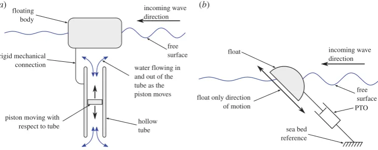
Figure 1.Section view schematic of a generic WEC reacting against water inertia (a) and side view schematic of the externally constrained sloped IPS buoy model tested by the University of Edinburgh (b).
is to maximize the amount of energy harvested from the waves while minimizing cost and ensuring survivability. Although it is not necessary where it is the most exploitable [8], wave energy resource is generally more energetic in deep water environments than in shallow, coastal areas. However, increased water depth makes it more difficult and more costly to design WECs whose power take-off (PTO) mechanisms react against the sea bed. In such situations, an alternative approach is to use an inertial mass for the PTO to react against. This reduces significantly mooring loads as the mooring system is then only used for station keeping and not as a reference for the PTO. For such WECs to produce a significant amount of power, the mass reference needs to be large. If it is to be part of the device structure, it will be associated with significant costs. One way to alleviate this issue is to use water inertia as the PTO reference. One generic WEC concept that corresponds to this approach consists of a fully submerged tube, open at both ends and fitted with a piston able to slide inside. The tube is rigidly mounted onto a floating body and is thus subjected to wave-induced motions. The piston, constrained by the inertia of the water inside the tube, provides a reaction for the PTO mechanism (figure 1a). Energy is thus extracted from the relative motion between the piston and the tube. This concept was originally pioneered by the Swedish company Inter Project Services AB whose device (the IPS buoy) was fitted with a vertical PTO tube as infigure 1a[9].
In the 1990s, the University of Edinburgh adapted the IPS buoy by tilting the axis of the PTO tube away from vertical in an attempt to use both heave and surge wave induced motions of the water particles. In a first scaled model experimental investigation, the motion of the float was externally constrained to a single degree of freedom which was a translation along a sloped direction as shown infigure 1b. The PTO was referenced to the sea bed. More information on this study can be found in [10,11].
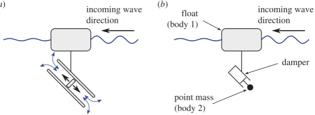
In a subsequent stage, a free-floating configuration was investigated. The main focus was to compare numerical modelling results with tank testing measurements [12,13]. In this configuration, the PTO was reacting against water inertia as depicted infigure 2a.
3
rspa.r
oy
alsociet
ypublishing
.or
g
Proc
.R.
Soc
.A
47
1
:2
01
50
23
[image:3.493.94.406.43.157.2]8
...
incoming wave direction
(a) (b)
damper
point mass (body 2)
incoming wave direction float
(body 1)
Figure 2.Section view schematics of a free-floating WEC reacting against water inertia (a) and against a point mass (b).
The paper first provides a detailed derivation of the numerical model which is then verified against numerical benchmark data. A parametric study and a multi-objective optimization are then carried out using a multi-linear regression method.
2. Numerical model derivation
The BEM package WAMIT was originally used in the offshore industry [14–17] but has more recently been used to model the behaviour of WECs [12,13,18–21].
The WEC described infigure 2b is modelled as a two-body system: the float (body 1) and the point mass (body 2). Only the former is subjected to hydrodynamic and hydrostatic loads. These are computed using WAMIT. The equations of motion of the system are expressed in the frequency domain using an Eulerian approach. The motion amplitudes of both bodies are considered small with respect to the cross-sectional dimensions of body 1 and with respect to wavelength. Equations of motion are linearized thus neglecting the terms of order higher than 1.
(a) System description and notations
The system is assumed to have a vertical plane of symmetry which is parallel to the direction of propagation of the waves. Consequently, motions of the system will be restricted to this plane. The only degrees of freedom considered are therefore surge, heave and pitch. Consequently, all forces and displacement components perpendicular to that plane are considered null. This also applies to all rotations and moment components whose axis are not perpendicular to that plane.
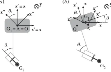
The coordinate systems and the notations used are summarized infigure 3in which the float (body 1) is shown in light grey and the point mass (body 2) is shown in darker grey.
R0=(O,x,y,z) is the global coordinate system,R1=(G1,x,y,z) is the body fixed coordinate
system associated with body 1,R2=(A,x,y,z) is the body fixed coordinate system associated
with body 2. G1is the centre of gravity of body 1 and G2the centre of gravity of body 2.m1and
m2are the masses of body 1 and 2, respectively. Point A is part of, in the sense that it moves with,
body 2. The positions of G1, G2and A are given inR0by the coordinate vectorsuG1,uG2anduA,
respectively, with
uG1=OG1=
⎛ ⎜ ⎜ ⎝
uG1
0
wG1
⎞ ⎟ ⎟
⎠, uG2=OG2=
⎛ ⎜ ⎜ ⎝
uG2
0
wG2
⎞ ⎟ ⎟
⎠ and uA=OA=
⎛ ⎜ ⎜ ⎝
uA
0
wA
⎞ ⎟ ⎟
⎠. (2.1)
When the system is at rest, G1 and A coincide with O andx andz coincide withx andz,
respectively. From the geometry of the system, at any time, vectors G1A andz are always parallel. This geometric constrain can be expressed by
4
rspa.r
oy
alsociet
ypublishing
.or
g
Proc
.R.
Soc
.A
47
1
:2
01
50
23
8
...
z¢ ∫z z¢ x¢¢ x¢
x z¢¢
z
G1∫A∫ O
G2
(a) (b)
G2 G1
O A
z¢¢ q° x¢¢
q° q°
q°
q
x¢∫x
[image:4.493.158.337.45.161.2]y y
Figure 3.Schematic of the two-body system with coordinate systems and notations. (a) The system is at rest, whereas in (b) it is in motion, away from its equilibrium position. The symbolrepresents the vectorybeing perpendicular to the plane of the sketch and pointing ‘into the page, away from the reader’.
The orientation ofR1and ofR2are given inR0by vectorsΩ1andΩ2, respectively, with
Ω1=
⎛ ⎜ ⎝ 0 θ 0
⎞ ⎟
⎠ and Ω2=
⎛ ⎜ ⎝
0 θ+θ0
0 ⎞ ⎟
⎠, (2.3)
whereθis the time varying angle betweenxandxandθ0is the fixed angle betweenzandz.
(b) Efforts applied to the system
The different stresses applied to the bodies are given using screw notations. An effort screw (or wrench)Sconsists of two vectorial quantities corresponding to a load: a forceFand an associated momentMP(expressed with respect to a point P) acting on the system:
S= FS
MS,P
P
.
For more details on this concept, see [22] (ch. 2 and 3) and [23].
Body 1 is subjected to the following stresses: weight, buoyancy, wave-induced loads and the linkage load applied by body 2 to body 1 through the damper. Some of the stresses induced by weight and buoyancy cancel each other out; the remaining hydrostatic loads are accounted for by a hydrostatic screw (H1). Wave-induced loads are split into hydrodynamic radiation loads (R1)
and hydrodynamic wave exciting loads (E1). The linkage load applied by body 2 to body 1 is
notedL2→1. Finally, the effort screw accounting for the external loads applied to body 1 is
T→1=E1+R1+H1+L2→1. (2.4)
The linkage between body 1 and body 2 is of cylinder type which means that it has two degrees of freedom: translation along thezdirection and rotation around that samezaxis. Given that the motion of the system is restricted to the (x,z) plane the latter degree of freedom is irrelevant. The linkage is fitted with a linear damper along thezdirection.
L2→1= MFL2→1
L2→1
O
= (FL2→1·x)x+Fdmp
ML2→1
O
, (2.5)
whereFdmpis the force from the damper given by
Fdmp= −α((u˙G1− ˙uA)·z)z, (2.6)
5
rspa.r
oy
alsociet
ypublishing
.or
g
Proc
.R.
Soc
.A
47
1
:2
01
50
23
8
...Hydrodynamic and hydrostatic quantities are computed by WAMIT in G1 but need to be
expressed with respect to O to solve the equations of motion. Let one considerH1in detail:
H1= MFH1
H1,G1
G1
= FH1
MH1,G1+OG1×FH1
O
, (2.7)
where OG1 is the vector from O to G1. Under the assumption of linearity, the magnitude of
OG1and ofFH1are first-order small quantities. Their product is, therefore, a second-order small
quantity and is thus negligible compared withMH1,G1andH1can be approximated as
H1≈ MFH1
H1,G1
O
. (2.8)
Similarly
R1≈ MFR1
R1,G1
O
and E1≈ MFE1
E1,G1
O
. (2.9)
Body 2 is subjected to the following stresses: weight and the linkage stress applied by body 1 to body 2 through the damper (L1→2). Since body 2 is a point mass without volume, it is not
subjected to any hydrodynamic loads. However, it is assumed that its weight is compensated by a force equal in magnitude and opposite in direction which could be assimilated to buoyancy. As explained in the introduction, body 2 is an approximation of the set consisting of the piston and the body of water contained in the tube (figure 2a). The set has a density which is dominated by that of water and is therefore neutrally buoyant. This assumption is necessary to ensure that the two-body system is stable at rest. If the weight of body 2 was not compensated the system would sink. In consequence, the effort screw accounting for the external loads applied to body 2 is reduced to
T→2=L1→2= −L2→1. (2.10)
(c) Dynamics equations
The dynamic screw concept (or acceleration screw) D of a body is similar to that of wrench introduced in §2b. It consists of two vectorial quantities: the linear acceleration and the angular acceleration (dynamic moment, notedδ) given with respect to a point.
For body 1,
D1= mδ1u¨G1 1,G1
G1
= m1u¨G1
δ1,G1+OG1×m1u¨G1
O
≈ m1u¨G1
δ1,G1
O
, (2.11)
where the Newton’s (or dot) notation is used for differentiation with respect to time. The approximation made in (2.11) is consistent with the assumption of linearity as explained for (2.8). Similarly for body 2,
D2= mδ2u¨G2 2,G2
G2
= m2u¨G2
δ2,G2+OG2×m2u¨G2
O
. (2.12)
Newton’s second law for the two-body system is expressed by
D1=T→1 and D2=T→2. (2.13)
Introducing the generalized displacement vectorξ
ξ= ⎛ ⎜ ⎜ ⎜ ⎜ ⎜ ⎝ ξ1 ξ2 ξ3 ξ4 ξ5 ⎞ ⎟ ⎟ ⎟ ⎟ ⎟ ⎠ = ⎛ ⎜ ⎜ ⎜ ⎜ ⎜ ⎝
uG1
6
rspa.r
oy
alsociet
ypublishing
.or
g
Proc
.R.
Soc
.A
47
1
:2
01
50
23
8
...(2.13) and (2.2) lead, in the frequency domain, to the following matrix equation whose detailed derivation is given in §A of the electronic supplementary material:
(−ω2(M+AH)+iω(BH+BS)+(CH+CS))ξ=EH, (2.15) whereωis the radian frequency and with
M= ⎛ ⎜ ⎜ ⎜ ⎜ ⎜ ⎝
m1 0 m2wG2r m2 0
0 m1 −m2uG2r 0 m2
0 0 I1,G1+m2(uG22r+wG22r) m2wG2r −m2uG2r
0 0 0 0 0
0 0 −m2uG2rcosθ0−m2wG2rsinθ0 −m2sinθ0 m2cosθ0
⎞ ⎟ ⎟ ⎟ ⎟ ⎟ ⎠ , (2.16)
AH=
⎛ ⎜ ⎜ ⎜ ⎜ ⎜ ⎝ 0 0 A 0 0 0 0
0 0 0 0 0
0 0 0 0 0
⎞ ⎟ ⎟ ⎟ ⎟ ⎟ ⎠
and BH=
⎛ ⎜ ⎜ ⎜ ⎜ ⎜ ⎝ 0 0 B 0 0 0 0
0 0 0 0 0
0 0 0 0 0
⎞ ⎟ ⎟ ⎟ ⎟ ⎟ ⎠ , (2.17)
BS=
⎛ ⎜ ⎜ ⎜ ⎜ ⎜ ⎝
0 0 0 0 0
0 0 0 0 0
0 0 0 0 0
0 0 0 0 0
αsinθ0 −αcosθ0 0 −αsinθ0 αcosθ0
⎞ ⎟ ⎟ ⎟ ⎟ ⎟
⎠, (2.18)
CH=
⎛ ⎜ ⎜ ⎜ ⎜ ⎜ ⎝ 0 0 C 0 0 0 0
0 0 0 0 0
0 0 0 0 0
⎞ ⎟ ⎟ ⎟ ⎟ ⎟ ⎠
and CS=
⎛ ⎜ ⎜ ⎜ ⎜ ⎜ ⎝
0 0 0 0 0
0 0 0 0 0
0 0 0 0 0
−cosθ0 −sinθ0 0 cosθ0 sinθ0
0 0 0 0 0
⎞ ⎟ ⎟ ⎟ ⎟ ⎟ ⎠ (2.19)
and EH= ⎛ ⎜ ⎝ E 0 0 ⎞ ⎟
⎠, (2.20)
uG2r and wG2r are the coordinates in R0 of G2 when the system is at rest. A, B andC are,
respectively, the added mass, hydrodynamic damping and hydrostatic 3×3 matrices computed by WAMIT.Eis wave exciting force 3×1 vector also computed by WAMIT.
3. Verification of the numerical model
The above derivation is relatively complex and it is important to ensure that no mistake has been left unspotted before using the model for optimization purposes. To do so, the model needs to be verified, to make sure that its outcomes are consistent with the underlying theory, so as to show that the model is doing what it is supposed to do [24]. This is done by comparing model results with benchmark computations from WAMIT. The results are also checked to ensure that they make physical sense.
(a) Comparison with benchmark data
7
rspa.r
oy
alsociet
ypublishing
.or
g
Proc
.R.
Soc
.A
47
1
:2
01
50
23
[image:7.493.63.434.44.265.2]8
...
0 0.5 1.0
1.5 surge
normalized amplitude
0 5 10
15 heave
0 5 10
15 pitch
1 2 3
–200 –100 0 100 200
period (s)
phase (°)
1 2 3
–200 –100 0 100
period (s)
1 2 3
–50 0 50 100
period (s)
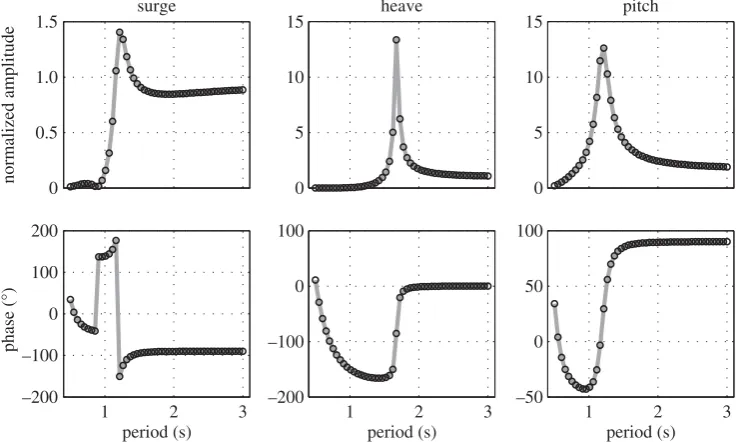
Figure 4.Comparisons between the response amplitude operators computed using only WAMIT with a modified mass matrix (grey line) and those calculated using equation (2.15) (black circle). Results are plotted as normalized amplitude (first row) and phase (second row) for the three degrees of freedom of interest.
WAMIT. The results from the model derived in this paper are therefore compared with those of a WAMIT single-body simulation but for which the mass properties of that single-body account for both the float and the point mass. The comparison is shown infigure 4. For this simulation, the float is a cylinder 0.5 m in diameter with a 0.5 m draft, its mass ism1=98.17 kg and its centre
of gravity is located on the cylinder axis, 0.4 m below the mean water level. The point mass is located 0.1 m below the centre of gravity of the float and its mass is a-tenth of that of the float:
m2=m1/10=9.82 kg. The damping coefficientα=109Nsm−1and the damper angleθ0=0◦. The
response amplitudes shown infigure 4are normalized by wave amplitude for surge and heave, and by wave slope (defined as arctan((2×wave amplitude)/(wave length/2))) for pitch.
The match between the two computations is excellent for all degrees of freedom, in terms of both amplitude and phase. The discrepancies do not exceed 7.67×10⁻⁴ in amplitude. Similar results are observed for any value of θ0. This contributes to build confidence in the model
derivation.
(b) Physical interpretation of simulations
Another way of providing reassurance in the model derivation is to gradually increase the values of the damping coefficient and of the mass of the point mass and to check that the evolution of the bodies response makes physical sense.
Figure 5 shows the amplitude of the heave response of the float (wG1) and of the point
mass (wA) for increasing values of the damping coefficientα, ranging from 1 to 1000 Nsm−1.
In comparison, the maximum radiation damping values of the float in surge and in heave are 333 Nsm−1and 15 Nsm−1, respectively.
8
rspa.r
oy
alsociet
ypublishing
.or
g
Proc
.R.
Soc
.A
47
1
:2
01
50
23
[image:8.493.63.433.43.270.2]8
...
0 5 10 15
Ω
wG
1
Ω
1.0 1.5 2.0 2.5
0 5 10 15
period (s)
Ω
wA
Ω
a= 1 Nsm–1
a= 10 Nsm–1
a= 25 Nsm–1
a= 100 Nsm–1
a= 1000 Nsm–1
Figure 5.Normalized amplitude of the heave displacement of the float (wG1) and of the point mass (wA) for various values of the damping coefficientα.
bodies, hence the similar heave response of the float and of the point mass. It can also be seen that as damping increases up to 100 Nsm−1, the amplitude of motion of the float at resonance is reduced whereas for the much higher damping value of 1000 Nsm−1, the float motion is large again. This can be explained by the fact that for damping values up to 100 Nsm−1, some of the energy in the system is dissipated by the damper which has the effect of reducing the float motion amplitude. For the highest damping value, however, there is hardly any relative motion between both bodies and very little energy is dissipated by the damper hence the large motion of the float. It can also be observed that the resonance period of the heave response increases withα. This can be physically explained by the fact that for low damping there is little coupling between the two bodies and the heave resonance periodThresof the float is mainly driven by the square
root of the ratio of its massm1plus heave added massahover the heave hydrostatic stiffnessch:
Thres∝
(m1+ah)/ch. However, for the highest damping value, the point mass can be considered integral to the float and is increasing its overall inertia. Given that the heave hydrostatic stiffness remains unchanged because it only depends on the geometry of the float, the heave resonance period increases:Thres∝
(m1+ah+m2)/ch. Variations inαaffect the system response in heave but not in surge or in pitch and that is why these latter degrees of freedom are not plotted in
figure 5. Given that the damper is vertical (θ0=0◦), the system is symmetrical about a vertical
plane which is perpendicular to the direction of propagation of the waves. In these conditions, the heave mode is decoupled from surge and pitch (see [25, p. 308] for more detail).
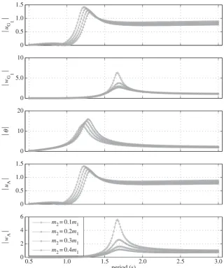
Infigure 6, the float geometry, its mass properties and the position of the point mass are the same as before. The damper is set vertical (θ0=0◦), the damping value is fixed (α=70 Nsm−1)
and the impact of increasing the massm2 of the point mass is shown. In heave, it can be seen
that the amplitude of the response of the point mass (wA) decreases with increasing values ofm2.
This makes physical sense given that the inertia of the point mass increases withm2whereas the
exciting force it experiences from the float via the damper remains largely unchanged. It can also be seen that the resonance period of the float response in heave (wG1) increases slightly
with m2. This is to be expected given that, in that mode of motion there is coupling between
the two bodies (via the damper) and that therefore an increase inm2tends to increase the heave
9
rspa.r
oy
alsociet
ypublishing
.or
g
Proc
.R.
Soc
.A
47
1
:2
01
50
23
[image:9.493.86.407.40.424.2]8
...
0 0.5 1.0 1.5
Ω
uG
1
Ω
0 5.0 10
Ω
wG
1
Ω
0 10 20
Ω
q
Ω
0 0.5 1.0 1.5
Ω
uA
Ω
0.5 1.0 1.5 2.0 2.5 3.0
0 2 4 6
period (s)
Ω
wA
Ω
m2= 0.1m1
m2= 0.2m1
m2= 0.3m1
m2= 0.4m1
Figure 6.Normalized amplitude of the displacements of the float (uG1,wG1andθ) and of the point mass (uAandwA) with the damper set vertical (θ0=0◦) andα=70 Nsm−1for various mass values of the point mass.
pitch (which are coupled), it can be observed that the resonance period also increases withm2but
more significantly than for heave. An increase inm2brings about an increase in the pitch moment
of inertia whereas the hydrostatic restoring torque stays constant. As for heave, this has the effect of increasing the resonance period. Moreover, given that the damper is vertical, the float and the point mass can be considered to be rigidly connected in surge and pitch and so the increase in
m2 impacts directly on float surge and pitch inertia and not in a ‘damped’ manner as it is the
case in heave.
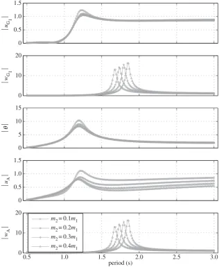
Figure 7shows the response of the system in the same conditions as infigure 6except that the damper is set horizontal (θ0=90◦). It can be seen that in this configuration, the heave motion of
the float (wG1) is the same as the heave motion of the point mass (wA). The impact of increased
m2on the heave resonance period is also more pronounced than infigure 6. This is to be expected
10
rspa.r
oy
alsociet
ypublishing
.or
g
Proc
.R.
Soc
.A
47
1
:2
01
50
23
[image:10.493.88.405.43.429.2]8
...
0 0.5 1.0 1.5
Ω
uG
1
Ω
0 10 20
Ω
wG
1
Ω
0 5 10 15
Ω
q
Ω
0 0.5 1.0 1.5
Ω
uA
Ω
0.5 1.0 1.5 2.0 2.5 3.0
0 10 20
period (s)
Ω
wA
Ω
m2= 0.1m1
m2= 0.2m1
m2= 0.3m1
m2= 0.4m1
Figure 7.Normalized amplitude of the displacements of the float (uG1,wG1andθ) and of the point mass (uAandwA) with the damper set horizontal (θ0=90◦) andα=70 Nsm−1for various mass values of the point mass.
In figures6and7, it can be seen that for long wave periods, the heave response amplitude of the float converges towards 1. This is consistent with the fact that in those circumstances, the heave wave loads are dominated by hydrostatic terms and the float therefore follows the wave surface (see [26, p. 134] for more details).
4. Parametric study and optimization
Figures 4–7and their interpretations provide a strong verification of the model and build the necessary confidence to be able to use the model reliably for parametric study and optimization purposes. The WEC configuration considered in this context consists of a point mass and of the same float as the one described in §3a. The mass properties of the float are fixed and are also described in §3a. The point mass is neutrally buoyant (as explained in §2b) and it is located along the vertical axis of the cylindrical float when the system is at rest.
11
rspa.r
oy
alsociet
ypublishing
.or
g
Proc
.R.
Soc
.A
47
1
:2
01
50
23
8
...
Table 1.Description and range of the parameters investigated for parametric study and optimization. The last column expresses the range of some of the parameters as a function of the float characteristics.
parameter symbol range range (relative value)
mass of the point mass m2 [19.6–117.8] kg [0.2m1–1.2m1]
. . . . vertical position of the point mass with
respect to the float
wG2r [−0.05 to−0.25] m [−0.1 to−0.5]×cylinder draft
. . . .
angle of the PTO θ0 [0–90]◦
. . . .
PTO damping α [100–1000] Nsm−1
. . . .
literature [27–30]. The present investigation focuses instead on PTO parameters with an emphasis on sloped motion.
No scale factor or any particular sea state are specified for the optimization. Doing so would have inevitably made the device size a key parameter for performance. This would have in turn shifted the focus of the study away from investigating purely the sloped PTO.
(a) Scopes and metrics
The parameters investigated and their range are given bytable 1. It should be noted that whilem2
was allowed to vary between [0.2m11.2m1], the optimization will only be conducted with values
ofm2≤m1. Extending the range ofm2 helps ensuring the validity of the models for values of
m2close tom1. The upperm2 value retained for the optimization (m2=m1) would correspond
to a tube whose internal volume is similar to that of the float. Although detailed engineering considerations are beyond the scope of this study, it is believed that this can be achieved, by spreading the reference body of water across several PTO tubes, for example. ThewG2r range was chosen so that the point mass is always below the centre of gravity of the float and therefore does not reduce its stability. It can be noticed that the range ofwG2r starts at−0.05 m, which is within the float and not below it. From an engineering point of view, this would correspond to having the PTO tube integrated to the float. ThewG2rlower limit was set to−0.5×cylinder draft as too large a distance between the float and the tube could be impractical from an engineering perspective.
Two metrics are considered to assess the performance of the WEC configurations explored. They are derived from the capture width ratio (CW) which corresponds to the ratio of the energy harvested by the WEC over the incoming wave energy available in a wave front whose width is equal to that of the device. More information on that concept can be found in [31].
The power captured by the WEC is calculated from the relative translational motion between the float and the point mass along the damper direction. The velocity associated with that motion is multiplied by the PTO damping force to obtain the captured power.
The two metrics used to assess WEC performance are the following.
Capture width area (CWarea) corresponds to the capture width ratio integrated over
the wave period spectrum. Physically, it gives an indication of the energy capture performance over the whole spectral range.
Mean capture width period(TmCW) is the mean of the wave period weighted by the capture
width ratio:
TmCW= 1
CWarea
spectrumCW(T)TdT, (4.1)
12
rspa.r
oy
alsociet
ypublishing
.or
g
Proc
.R.
Soc
.A
47
1
:2
01
50
23
8
...
good performance in long waves is advantageous because it potentially increases power production while keeping the float size, and therefore to some extends its cost, constant.
(b) Method
(i) Generation of data
Four thousand WEC configurations are generated by randomly selecting 4000 combinations of the four parameters within the range specified intable 1. The performance and body motions of each configuration are then computed over a 0.5 to 4 s wave period range using the equations derived in §2c.
The amplitude of motions predicted by linear BEM can be non-physically large. This is mainly due to the fact that potential flow theory, on which BEM is based, does not account for viscous effects which damp body motion. Unrealistically large body motions can lead to erroneous predictions of WEC power absorption which would in turn distort the PTO optimization. To circumvent this issue, configurations exhibiting normalized motion amplitudes (as defined in §3a) higher than 10 are discarded. This way, from an initial set of 4000 randomly generated WEC configurations, 600 are typically retained.
(ii) Scores
The optimization process with respect to each of the metrics defined in §4a taken individually could lead to conflicting requirements. A way around this issue is to combine the different metrics in a single objective function leading to a single score. This is done as follows. For a given WEC configuration, each metric is normalized by its maximum value achieved over the full set of retained configurations. The score of each configuration is then defined as the weighted sum of the normalized metrics, keeping the sum of the weight equal to 1. This ensures that scores are kept within the [0 1] range. This approach makes it possible to control and investigate the influence of each metric on the overall score. Three weight combinations are defined as part of the optimization process:
score20=0.2 TmCW
max(TmCW)+0.8
CWarea
max(CWarea) (4.2)
score40=0.4 TmCW
max(TmCW)+0.6
CWarea
max(CWarea) (4.3)
and score50=0.5 TmCW
max(TmCW)+0.5
CWarea
max(CWarea) (4.4)
(iii) Optimization
The process of optimization consists first in fitting an analytical model to the observed score distribution. The parameters of the model (defined in table 1) are the variables to optimize. The scores and associated variables (m2,wG2r,θ0andα) are imported into the statistical analysis
package R [32].
(c) Results
(i) Experimental plan
13
rspa.r
oy
alsociet
ypublishing
.or
g
Proc
.R.
Soc
.A
47
1
:2
01
50
23
[image:13.493.90.406.40.450.2]8
...
20 40 60 80 100 120
−0.25 −0.20 −0.15 −0.10 −0.05
m2 as % of m1
wG
2
r
(m)
20 40 60 80 100 120
−80 −60 −40 −20 0
m2 as % of m1
q0
(°)
20 40 60 80 100 120
200 400 600 800 1000
m2 as % of m1
a
(Nsm
−1
)
−0.25 −0.20 −0.15 −0.10 −0.05 −80
−60 −40 −20 0
w G2r (m)
q0
(°)
−0.25 −0.20 −0.15 −0.10 −0.05 200
400 600 800 1000
w G2r (m)
a
(Nsm
−1
)
−80 −60 −40 −20 0
200 400 600 800 1000
q0 (°)
a
(Nsm
−1
)
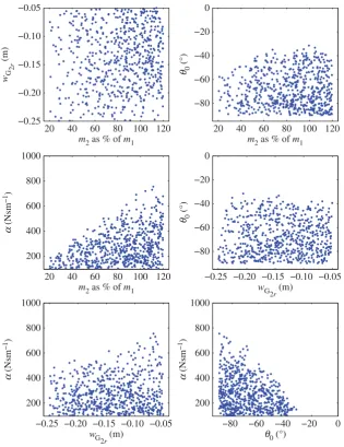
Figure 8.Resulting experimental plan obtained after excluding configurations for which motion amplitudes were dimmed unrealistic.
It can be noted that the nearest angle to vertical included in the experimental plan is about θ0= −30◦. Indeed, for PTO angles closer to vertical, the normalized pitch motion exceeds 10.
Although these large pitch responses are partly due to the numerical model neglecting viscous and radiation damping on the PTO structure, it also reflects a real physical pitch instability exhibited by some free-floating WECs with similar geometry and a vertical PTO [33]. In this context, a sloped PTO direction brings beneficial damping to the pitch motion.
(ii) R model
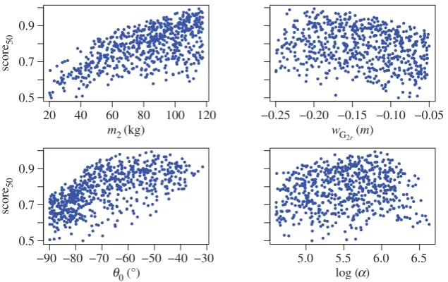
Figure 9 shows score50 plotted as a function of the four variables. log(α) is used instead ofα
as it provides a better spread of the points with respect to that variable. It can be seen from these plots that linear trends of score50 with respect tom2 andwG2r can be expected, whereas at least square laws should be considered to model the evolution of score50 with respect toθ0
14
rspa.r
oy
alsociet
ypublishing
.or
g
Proc
.R.
Soc
.A
47
1
:2
01
50
23
[image:14.493.90.408.39.239.2]8
...
20 40 60 80 100 120
0.5 0.7 0.9
m2 (kg)
score
50
−0.25 −0.20 −0.15 −0.10 −0.05 wG
2r (m)
−90 −80 −70 −60 −50 −40 −30 0.5
0.7 0.9
q0 (°)
score
50
5.0 5.5 6.0 6.5
log (a)
Figure 9.score50with respect to the four parameters to optimize. log(α) is used instead ofαas it was found to better spread the data and to lead to a better model fit.
The model is fitted to the distribution in R using the following call:
logModel <- lm(score50 ~ {I}(theta0^2) + I((log(alpha))^2) + (theta0 + m2 + alpha + wG2r)^2).
This model considers a square term forθ0and log(α), as well as linear terms for the four variables
and their possible interactions.
The model is then simplified to remove the non-significant terms. The final model fitted to score50is presented in equation (4.5).
score50(m2,θ0,α,wG2r)= −1.614−0.1641e−3θ02−0.06479 log(α)2−0.01809θ0
+0.2134e−2m2+0.6276 log(α)+0.2093e−4θ0m2−0.3209e−3θ0log(α)
−0.5970e−2θ0wG2r+0.4651e−3m2log(α)+0.2867e−2m2wG2r
−0.2419 log(α)wG2r. (4.5)
The summary of the models and the check plots are presented in §B of the electronic supplementary material. It can be observed that the model is not perfect, as the residuals appear to depart from normality. However, the fitted model is not to be used for extrapolation but solely for interpolation, and to reveal trends about the influence of each parameter. Ther2-value associated to the model is 0.9674 and its residual standard error is 0.01909, which is thought to be acceptable given the observed dispersion.
Similar models were fitted to score20and score40. These are summarized in §B of the electronic
supplementary material.
(iii) Optimization results
Optimizing the WEC now corresponds to finding the combination of parameters maximizing the model scores. For score50, it can be observed that the model derivative with respect tom2
15
rspa.r
oy
alsociet
ypublishing
.or
g
Proc
.R.
Soc
.A
47
1
:2
01
50
23
[image:15.493.90.405.46.235.2]8
...
−90 −80 −70 −60 −50 −40 −30
0.4 0.6 0.8 1.0
score
50
q0 (°)
a= 150 Nms−1
a optimum
a= 600 Nms−1
0 100 200 300 400 500 600 700 800 900 1000
0.4 0.6 0.8 1.0
score
50
a (Nms−1)
q0= −70°
q0 optimum
q0= −35°
(b) (a)
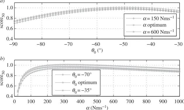
Figure 10.Variation of the analytical model fitted to score50with respect toθ0for three levels of PTO damping (a) and with respect toαfor three values ofθ0(b). For both graphsm2andwG2rare set to optimum.
The optimal values forθ0andαare found by solving the following system of equations:
∂score50(m1,θ0,α,−0.25)
∂θ0 =0
∂score50(m1,θ0,α,−0.25)
∂α =0
⎫ ⎪ ⎪ ⎬ ⎪ ⎪
⎭. (4.6)
Solving (4.6) leads toθ0= −49.97◦andα=325.76 Nsm−1. These values are within the bounds
shown infigure 8. For this set of values, the score obtained from the analytical model is larger than 1: score50(m2=m1,θ0= −49.97,α=325.76,wG2r= −0.25)=1.011230516. By inputting these values of parameters to the hydrodynamic model derived in §2c, score50=0.9670 is obtained.
By comparison, the highest score50in the randomly generated data set withm2≤m1is score50=
0.9473. This means that the optimization method used has provided a combination of parameters with a better score than the one associated with any of the randomly generated configurations.
It is interesting to look at the sensitivity of score50toθ0andα.Figure 10shows the variation
of the analytical model as a function ofθ0for three levels of PTO damping and as a function ofα
for three values ofθ0. It can be observed that the model shows a strong sensitivity toθ0. On the
top plot, score50increases rapidly as the PTO direction departs from horizontal towards a sloped
angle, which suggests strong benefit in inclining the PTO direction. Low values ofαare associated with very low scores. However, as soon as values over 100 are reached, the sensitivity toαis less pronounced. This suggests that it should be possible to vary significantly the PTO damping if required (e.g. for stability reasons or to limit the damper motion) without impacting too much on performance.
Finally, the influence of the weighting factors used for the definitions of the scores on the optimization results is investigated. The optimal values form2andwG2rare identical in the three
scoresdefined in §4b(ii).Table 2gives a summary of the optimum configurations corresponding
to the three different scores.
It can be observed that the optimal θ0 is very similar for the three different scores. This is
16
rspa.r
oy
alsociet
ypublishing
.or
g
Proc
.R.
Soc
.A
47
1
:2
01
50
23
[image:16.493.87.409.41.153.2] [image:16.493.64.439.235.392.2]8
...
0.5 1.0 1.5 2.0 2.5 3.0 3.5 4.0
0 0.2 0.4 0.6 0.8 1.0
period (s)
capture width ratio
score50
score40
score20
Figure 11.Capture width ratios plotted against wave period for the threescoresinvestigated.
Table 2.Summary of the optimal configurations found for the three different scores defined in §4b(ii). From the left to the right, relative importance of CWareais increasing and relative importance ofTmCW is decreasing.
optimum score50 optimum score40 optimum score20
m2 m1 m1 m1
. . . .
wG2r −0.25 −0.25 −0.25
. . . .
θ0 −49.96 −49.87 −49.80
. . . .
α 325.76 326.95 293.11
. . . .
CWarea 1.573 1.573 1.569
. . . .
TmCW 1.808 1.808 1.801
. . . .
score50 0.9668 0.9669 0.9639
. . . .
score40 0.962 0.9621 0.9592
. . . .
score20 0.9523 0.9524 0.9498
. . . .
problematic. Additionally, as can be seen infigure 10, the sensitivity of thescorestoαis low in the [250−400] Nsm−1range, and the variability seen intable 2might therefore not be in fact very significant.
Table 2shows the capture width area, the mean capture width period and the different scores for each optimum. From these data, it can be seen that some configurations optimized for a given score perform less well for that score (by a tiny amount) than configurations optimized for a different score. For example, the optimum solution for score20would be expected to have a higher
score20than the two other solutions but that is not the case. As the three solutions are very close,
these discrepancies are thought to be due to noise in the optimization process. These discrepancies would be less likely to occur if the two optimization metrics did not lead to similar results as is the case here.
17
rspa.r
oy
alsociet
ypublishing
.or
g
Proc
.R.
Soc
.A
47
1
:2
01
50
23
8
...
5. Conclusion
The concept of inclining the PTO axis of a free-floating WEC reacting against water inertia has been investigated using numerical modelling. The shape of the WEC has deliberately been kept to that of a simple vertical axis circular cylinder and the study has focused on PTO parameters. The derivation of the numerical modelling has been presented in detail. The thorough validation of that model has been carried out by ensuring that the results made physical sense and by comparing these with benchmark numerical data. This successful validation has built the necessary confidence into the model so that it could reliably be used for the parametric study and the optimization which has investigated the impact of the mass of the point mass, of its vertical position, of the angle of the PTO damper and of the damping value on the WEC performance. A multi-linear regression method has been used to find the set of parameters which provides the best performance in terms of linear combinations of capture width area and mean capture width period. Four thousand WEC configurations have been generated in that process. The optimum values form2is the maximum of the range considered, i.e.m2=m1. ForwG2rit is the lowest value of the range:wG2r= −0.25 m. For the PTO angle and damping, the optimum values vary slightly with the score chosen. It is respectively between 293 and 327 Nms−1and around 50◦.
Given the simplicity of the WEC shape and the fact that the numerical modelling technique used is frequency domain BEM, computations for each configuration was quick. This makes it possible to compute the performance of a large number of configurations. In that context, it would have been possible to identify a best performing configuration by carrying out a systematic exploration of the parametric domain with a fine parametric resolution. It should, however, be noted that the fitting of the analytical model and the subsequent optimization did yield some performance improvement over the best of the 4000 initial cases, which is already a large number of configurations. But perhaps more importantly, the optimization approach used here has provided an understanding of the impact of each parameter on the device performance and behaviour and this could not have been achieved with a systematic ‘brute-force’ optimization.
The parametric study shows, in a comprehensive manner, the clear advantage of an inclined PTO direction versus a vertical one. This is physically due to the fact that inclined configurations exploit resonance in both heave and pitch, thus widening the period range over which high capture width ratios are observed. These fundamental results pave the way for exploring further WEC concepts featuring sloped PTOs.
Data accessibility. This article is solely based on numerical modelling and has therefore no data associated with it. Authors’ contributions. G.P. led this study, led the development of the numerical method and drafted the manuscript; R.P. conducted the optimization process and helped drafting the manuscript; G.V. took part in the development of the numerical method. All authors gave final approval for publication.
Competing interests. At the time of submitting this manuscript, none of the authors had vested interests in the promotion of WEC technologies based on slopped PTO.
Funding. This work was supported by the UK Engineering and Physical Sciences Research Council (R35500) and by the UK Department of Trade and Industry (V/06/00184/00/00).
Acknowledgements. The authors thank Prof. Stephen Salter of the University of Edinburgh for introducing them to the concept sloped WEC.
References
1. Salter S. 1974 Wave power.Nature249, 720–724. (doi:10.1038/249720a0)
2. Evans D. 1976 A theory for wave-power absorption by oscillating bodies.J. Fluid Mech.77, 1–25. (doi:10.1017/S0022112076001109)
3. Henderson R. 2006 Design, simulation, and testing of a novel hydraulic power take-off system for the pelamis wave energy converter. Renew. Energy 31, 271–283. (doi:10.1016/j.renene. 2005.08.021)
18
rspa.r
oy
alsociet
ypublishing
.or
g
Proc
.R.
Soc
.A
47
1
:2
01
50
23
8
...
5. Yemm R, Pizer D, Retzler C, Henderson R. 2012 Pelamis: experience from concept to connection.Phil. Trans. R. Soc. A370, 365–380. (doi:10.1098/rsta.2011.0312)
6. Heath TV. 2012 A review of oscillating water columns.Phil. Trans. R. Soc. A370, 235–245. (doi:10.1098/rsta.2011.0164)
7. Titah-benbouzid H, Benbouzid M. 2015 Ocean wave energy extraction: up-to-date technologies review and evaluation. InProc. of the 2014 IEEE PEAC, pp. 338–342. Shanghai, China: IEEE.
8. Folley M, Whittaker TJ. 2009 Analysis of the nearshore wave energy resource.Renew. Energy
34, 1709–1715. (doi:10.1016/j.renene.2009.01.003)
9. Bergdahl L. 1992 Review of research in Sweden. InWave energy R&D workshop, pp. 129–136. Cork, Ireland: Commission of the European Communities.
10. Salter S, Lin C-P. 1995 The sloped IPS wave energy converter. In2nd European Wave Energy Conf., Lisbon, Portugal, pp. 337–344. Nantes, France: EWTEC.
11. Salter S, Lin C-P. 1998 Wide tank efficiency measurements on a model of the sloped IPS buoy. In3rd European Wave Energy Conf., Patras, Greece, pp. 200–206. Nantes, France: EWTEC. 12. Payne GS, Taylor JR, Bruce T, Parkin P. 2008 Assessment of boundary-element method for
modelling a free-floating sloped wave energy device. Part 1: numerical modelling.Ocean Eng.
35, 333–341. (doi:10.1016/j.oceaneng.2007.10.006)
13. Payne GS, Taylor JR, Bruce T, Parkin P. 2008 Assessment of boundary-element method for modelling a free-floating sloped wave energy device. Part 2: experimental validation.Ocean Eng.35, 342–357. (doi:10.1016/j.oceaneng.2007.10.008)
14. Newman J, Sclavounos P. 1988 The computation of wave loads on large offshore structures. InConf. on the Behaviour of Offshore Structures (BOSS ’88), vol. 2, Trondheim, Norway, pp. 605–622. New York, NY: Elsevier.
15. Newman J, Lee C-H. 1992 Sensitivity of wave loads to the discretization of bodies. InConf. on the Behaviour of Offshore Structures(BOSS ’92), vol. 1, London, UK, pp. 50–64. New York, NY: Elsevier.
16. Lee C-H, Maniar H, Newman J, Zhu X. 1996 Computations of wave loads using a B-spline panel method. In21st Symp. on naval hydrodynamics, Trondheim, Norway, pp. 75–92. Washington, DC: National Academies of Science.
17. Birk L, Clauss G. 2002 Parametric hull design and automated optimization of offshore structures. In10th Int. Congress of the Int. Maritime Association of the Mediterranean, Hellas,
Greece.
18. Folley M, Whittaker T. 2013 Validating a spectral-domain model of an OWC using physical model data.Int. J. Mar. Energy2, 1–11. (doi:10.1016/j.ijome.2013.05.003)
19. De Backer G, Vantorre M, De Beule K, Beels C, De Rouck J. 2009 Experimental investigation of the validity of linear theory to assess the behaviour of a heaving point absorber at the belgian continental shelf. In28th Int. Conf. on Ocean, Offshore and Arctic Engineering(OMAE), vol. 4, no. PART B, Honolulu, HI, pp. 1013–1020.
20. Delauré Y, Lewis A. 2003 3D hydrodynamic modelling of fixed oscillating water column wave power plant by a boundary element methods.Ocean Eng. 30, 309–330. (
doi:10.1016/S0029-8018(02)00032-X)
21. Lee C-H, Newman J, Nielsen F. 1996 Wave interactions with an oscillating water column. In
6th Int. Offshore and Polar Eng. Conf., vol. 1, Los Angeles, CA, pp. 82–90.
22. Featherstone R. 1987 Robot dynamics algorithms. Dordrecht, The Netherlands: Kluwer Academic Publishers.
23. Ball R. 1900A treatise on the theory of screws. Cambridge, UK: Cambridge University Press. 24. Standing R. 1991 The verification and validation of numerical models, with examples taken
from wave diffraction theory, wave loading and response. InIUTAM Symp. Dynamics of Marine Vehicles and Structures in Waves(eds W Price, P Temarel, A Keane), pp. 263–278. New York, NY: Elsevier.
25. Newman J. 1977Marine hydrodynamics. Cambridge, MA: MIT Press.
26. Falnes J. 2002Ocean waves and oscillating systems. Cambridge, UK: Cambridge University Press. 27. Babarit A, Clément A, Gilloteaux J-C. 2005 Optimization and time-domain simulation of the searev wave energy converter. In24th Int. Conf. on Offshore Mechanics and Arctic Engineering
(OMAE), Halkidiki, Greece.
19
rspa.r
oy
alsociet
ypublishing
.or
g
Proc
.R.
Soc
.A
47
1
:2
01
50
23
8
...
29. McCabe A. 2013 Constrained optimization of the shape of a wave energy collector by genetic algorithm.Renew. Energy51, 274–284. (doi:10.1016/j.renene.2012.09.054)
30. Gomes RPF, Henriques JCC, Gato LMC, Falcão AFO. 2012 Hydrodynamic optimization of an axisymmetric floating oscillating water column for wave energy conversion.Renew. Energy44, 328–339. (doi:10.1016/j.renene.2012.01.105)
31. Evans D. 1978 The oscillating water column wave-energy device. J. Inst. Math. Appl. 22, 423–433. (doi:10.1093/imamat/22.4.423)
32. R Core Team. 2012 R: a language and environment for statistical computing. Vienna, Austria: R Foundation for Statistical Computing. Seehttp://www.R-project.org/.