Performance of downscaled regional climate simulations using a variable-resolution regional climate model : Tasmania as a test case

Performance of downscaled regional climate simulations

using a variable-resolution regional climate model:

Tasmania as a test case

Stuart Corney,1Michael Grose,1,2James C. Bennett,3,4Christopher White,1Jack Katzfey,5 John McGregor,5Greg Holz,1and Nathaniel L. Bindoff1,3,5

Received 24 April 2013; revised 30 July 2013; accepted 2 October 2013; published 8 November 2013.

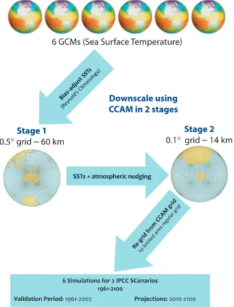
[1] In this study we develop methods for dynamically downscaling output from six general circulation models (GCMs) for two emissions scenarios using a variable-resolution atmospheric climate model. The use of multiple GCMs and emissions scenarios gives an estimate of model range in projected changes to the mean climate across the region. By modeling the atmosphere at a veryfine scale, the simulations capture processes that are important to regional weather and climate at length scales that are subgrid scale for the host GCM. Wefind that with a multistaged process of increased resolution and the application of bias adjustment methods, the ability of the simulation to reproduce observed conditions improves, with greater than 95% of the spatial variance explained for temperature and about 90% for rainfall. Furthermore, downscaling leads to a significant improvement for the temporal distribution of variables commonly used in applied analyses, reproducing seasonal variability in line with observations. This seasonal signal is not evident in the GCMs. This multistaged approach allows progressive improvement in the skill of the simulations in order to resolve key processes over the region with quantifiable improvements in the correlations with observations.

Citation: Corney, S., M. Grose, J. C. Bennett, C. White, J. Katzfey, J. McGregor, G. Holz, and N. L. Bindoff (2013), Performance of downscaled regional climate simulations using a variable-resolution regional climate model: Tasmania as a test case,J. Geophys. Res. Atmos.,118, 11,936–11,950, doi:10.1002/2013JD020087.

1. Introduction

[2] Anthropogenic climate change is likely to have

wide-ranging impacts across the spectrum of natural and human sectors. Responding and adapting to these impacts will be a sig-nificant challenge for governments, businesses, and individuals. As such, there is great interest in obtaining projections of cli-mate that can be used to inform responses and adaptation mea-sures at a local scale. Analysis of output from an ensemble of coupled general circulation models (GCMs) using a range

of future emissions scenarios is currently the most useful tech-nique we have to estimate likely changes to the climate system resulting from an enhanced greenhouse effect.

[3] Twenty-three GCMs were published in the Coupled Model

Intercomparison Project Phase 3 (CMIP3) archive [Meehl et al., 2007a] and were considered in the Intergovernmental Panel on Climate Change (IPCC) Fourth Assessment Report chapters on global changes [Meehl et al., 2007b] and regional changes [Christensen et al., 2007]. The analysis of multiple GCMs allows for the production of a “central estimate” of future climate change for a given scenario by examining the multimodel mean change in key variables (such as tempera-ture and rainfall) as well as providing an estimate of the model uncertainty in these climate variables through the spread of the models. However, the output from GCMs is currently of

insuf-ficient spatial resolution to illustrate the regional detail of projected climate change and its potential impacts at a scale relevant to decision makers [Christensen et al., 2007]. GCM output available through the CMIP3 website has horizontal resolutions on the order of 200–300 km. Coarse spatial reso-lution has an inevitable effect on the temporal character of outputs, where localized and short-duration events are poorly resolved. The coarse spatial resolution and temporal defi cien-cies of GCMs limit the effectiveness of GCM model output in providing useful information at the regional scale. Local climate change impact assessments often rely on models of hydrological, agricultural, or ecological systems to quantify

1_{Antarctic Climate and Ecosystems Cooperative Research Centre,}

University of Tasmania, Hobart, Tasmania, Australia.

2_{CSIRO Marine and Atmospheric Research, Aspendale, Victoria, Australia.} 3

Institute for Marine and Antarctic Studies, University of Tasmania, Hobart, Tasmania, Australia.

4

CSIRO Land and Water, Highett, Victoria, Australia.

5_{Centre for Australian Weather and Climate Research, CSIRO Marine}

and Atmospheric Research, Aspendale, Victoria, Australia.

Corresponding author: S. P. Corney, Antarctic Climate and Ecosystems Cooperative Research Centre, University of Tasmania, Private Bag 80, Hobart, Tas 7001, Australia. (Stuart.Corney@acecrc.org.au)

the changes [Hughes, 2003;Ines and Hansen, 2006;Fowler et al., 2007;Chiew et al., 2009]. These models require inputs such as rainfall, evaporation, and temperature, often at daily and subdaily time steps that account for processes of climate and climate change relevant to the site of interest. This level of regional detail in the projected climate change signal requires downscaling of GCM outputs. Downscaling can be done using statistical models (see review of statistical methods such as Fowler et al. [2007]) or through dynamical down-scaling using regional climate models (RCMs).

[4] Feser et al. [2011] have shown that dynamical RCMs

add value to GCM results when simulating current climate, particularly in mountainous or coastal regions where meso-scale phenomena are important. The higher resolution of RCMs gives the potential to resolve processes such as synop-tic systems, narrow jet cores, cyclogenesynop-tic processes, gravity waves, mesoscale convective systems, sea breezes, and extreme weather systems that are poorly resolved in GCMs [Mearns et al., 2003]. However, RCMs inherit biases from the host model and introduce new uncertainties associated with the downscaling model itself [Foley, 2010]. Dynamical RCMs can be divided into two broad categories: limited-area RCMs and variable-resolution global atmospheric models (we regard a variable-resolution global model that has a re-gion of particular interest at much higher resolution than the rest of the globe as a regional climate model). Limited-area RCMs use a higher-resolution grid over a subset of the globe and thus require lateral (atmospheric) boundary conditions from a host (or parent) GCM. There are various possible configurations of a variable grid, and here we exam-ine a stretched grid with a higher resolution over the area of in-terest. The use of stretched-grid RCMs is less common than limited-area RCMs, even though these models have been shown to simulate rainfall and related processes realistically at a range of scales and locations [e.g., Berbery and Fox-Rabinovitz, 2003;Boe et al., 2007]. Stretched-grid RCMs have no lateral boundaries and accordingly do not suffer from the problems associated with lateral boundaries in limited area models [Fox-Rabinovitz et al., 2008], while still providing

re-finement of the large-scale features of the host GCM in the high-resolution area of interest. Crucially for our study, a stretched-grid RCM can be configured to be forced only through the lower boundary (i.e., surface temperature, see for exampleEngelbrecht et al. [2009]) enabling the possi-bility of bias-correcting global climate model sea surface temperature before downscaling (see section 3.2 below).

[5] This study presents downscaled climate projections for

Tasmania, Australia. The aim of this study is to provide very high resolution climate projections for use in applied analyses that will inform the Tasmanian community of impacts of projected changes on the regional climate of Tasmania up to 2100, including changes to water availability, changes to hydropower generation capacity, changes to extreme events, and changes to agricultural productivity. Accordingly, the method we chose for this study had to produce plausible projec-tions of future climate with veryfine regional detail. Dynamical downscaling of coupled ocean-atmosphere GCMs can show the regional detail of projected climate changes incorporating the effect of Tasmania’s complex topography and range of climate drivers, to thereby provide a clearer picture of regional variations and impacts of projected climate change. The model-ing program dynamically downscaled six GCMs to a final

resolution of about 10 km over Tasmania. Two emissions sce-narios were used to represent a range of plausible future emis-sions from the IPCC Special Report on Emisemis-sions Scenarios (SRES) [Nakicenovic and Swart, 2000], and the simulations covered the period 1961 to 2100. The model output has been used to inform the Tasmanian government’s response to climate change and 29 local councils of the likely regional changes to climate and primary producers across a range of industries.

2. Study Site

[6] Tasmania is Australia’s island state, located off the

southeast corner of the continent. Tasmania’s topography is mountainous in much of the south, west, and central, causing a sharp east-west rainfall gradient from more than 3000 mm annually in the west to less than 500 mm in the eastern lowlands [Bureau of Meteorology, 2008]. Mean daily maximum temper-atures range from 8.6°C on Mount Read in western Tasmania to 18.3°C at Friendly Beaches on Tasmania’s east coast. The southwest of Tasmania is home to a World Heritage area of high conservation value. Agriculture is an important industry in the drier eastern regions;Post et al. [2012] note that there are plans to develop significant new irrigation infrastructure in eastern Tasmania in light of declining yields in the Murray-Darling Basin and southwest Western Australia.

[7] The relationship of rainfall variability to mean circulation

and remote drivers of rainfall vary considerably across the rela-tively small area of Tasmania [Risbey et al., 2009].Christensen et al. [2007] showed that Tasmania lies near the border between the subtropics, where most CMIP3 models show that annual rainfall is projected to decrease, and the high latitudes, where mean annual rainfall is projected to increase with a warming climate. The placement and resolution of this boundary is especially relevant to the projected mean annual rainfall of Tasmania, as it determines the sign of the projected change for locations within the state. Tasmania’s diverse geography and varied climate make it particularly difficult to assess the re-gional impacts of climate change on temperature, rain, and other climate variables when relying solely on low-resolution GCMs.

3. Downscaling Methods and Approach

3.1. GCM Selection

[8] There have been several assessments of GCM

or inSmith and Chandler[2010], but is also included as the most recent version of the Australian GCM available at the commencement of our study. The models were chosen to rep-resent a range of projections in the 23 GCMs andGrose et al. [2013] have shown that mean rainfall changes and model agreement projected by the mean of the six GCMs chosen for this study are broadly similar to rainfall changes projected by the mean of the 23 CMIP3 GCMs over Australia. Note that GFDL-CM2.0 and GFDL-CM2.1 can be regarded as separate, independent GCMs due to their different dynamical cores, ocean time-stepping schemes, and lateral viscosity. In line with IPCC recommendations [IPCC, 2007], we chose a high (A2) and a low (B1) emissions scenario to sample a range of plausible emissions scenarios for unmitigated climate change. [9] The choice of six GCMs and two SRES emissions

scenarios gives a total of 12 representations of climate for Tasmania, including 47 years of hindcast (1961–2007) and over 90 years of projected future climate (2008–2100).

3.2. Conformal Cubic Atmospheric Model Configuration and Downscaling Method

[10] To perform the dynamical downscaling, we use the

Conformal Cubic Atmospheric Model (CCAM) from CSIRO [McGregor and Dix, 2001;McGregor, 2005;McGregor and Dix, 2008]. CCAM has been used for regional climate studies in Australia [Nunez and McGregor, 2007;Watterson et al., 2008;McGregor and Nguyen, 2009;Nguyen and McGregor, 2009a, 2009b; Frost et al., 2011] and internationally [Lal et al., 2008;Engelbrecht et al., 2009;Nguyen and McGregor, 2009b; Katzfey et al., 2010; Feng et al., 2011]. CCAM is a global atmospheric climate model that uses a conformal cubic grid. CCAM is configured to use a stretched grid by utilizing the Schmidt [1977] transformation of the coor-dinates with higher resolution in areas of interest and lower resolution elsewhere.

[11] CCAM uses a semi-Lagrangian advection scheme and

semi-implicit time integration with an extensive set of physical parameterizations in a hydrostatic formulation. The GFDL

parameterizations for long-wave and short-wave radiation [Lacis and Hansen, 1974;Schwarzkopf and Fels, 1991] were used, with interactive cloud distributions determined by the liquid and ice water scheme ofRotstayn[1997]. The simu-lations used a stability-dependent boundary layer scheme based on Monin-Obukhov similarity theory [McGregor et al., 1993]. The canopy scheme described byKowalczyk et al. [1994] was employed with six layers for soil temp-erature, six for soil moisture, and three for snow. CCAM’s cumulus convection scheme with both downdrafts and detrainment, as well as mass-flux closure, is described by

McGregor [2003]. The simulations used fixed vegetation and soil type.

3.3. Lower Boundary Forcing: SST Bias Adjustment

[12] Coupled GCMs typically have biases in their

simu-lation of the mean current climate [Randall et al., 2007], including their simulation of mean SSTfields. In particular, the SST “cold tongue” bias along the equatorial Pacific [Lin, 2007] causes some challenging issues for the climate modeling community [Mechoso et al., 1995]. This bias pro-duces air-sea fluxes that affect the atmospheric model and cause deficiencies in the simulated climate. To ameliorate these problems, we adjust SST biases in the parent GCMs before downscaling. The global extent of CCAM allows for the model to be run without lateral boundary conditions and thus without any atmospheric forcing. CCAM can be run with only lower boundary conditions since the majority of the long-term climate variability and change signal is repre-sented in SST patterns, and the atmosphere quickly adjusts to the underlying surface forcings, a principle that underlies the Atmospheric Model Intercomparison Project (AMIP) set of experiments [Gates et al., 1998]. This means bias-adjusting SST will not produce inconsistencies with atmo-spheric variables. In this configuration, the bottom boundary conditions are SSTfields and sea ice concentrations, while the land surface and sea ice temperatures are dynamically modeled by CCAM. We calculate SST biases for each GCM

−150 −100 −50 0 50 100 150

−80 −60 −40 −20 0 20 40 60 80

(a) Mean SST

−150 −100 −50 0 50 100 150

−80 −60 −40 −20 0 20 40 60 80

(b) Cross−validated bias−corrected SST

−10 −7 −4 −2.5 −1 1 2.5 4 10

Bias (°C)

−1 −0.7 −0.4−0.25−0.1 0.1 0.25 0.4 0.7 1

Bias (°C)

7

and for each calendar month by subtracting mean GCM SSTs from mean observed [Reynolds, 1988] SSTs:

SSTbias¼SSTOBSSSTGCM; (1)

where SSTOBSis mean observed SST, SSTGCMis mean sim-ulated SST for the period that observations are available (1960–2000), and SSTbiasis the bias for each month. We then add the bias to the GCM SST to create bias-adjusted SST and use bias-adjusted SSTfields to force CCAM. Raw monthly mean sea ice concentrations were taken directly from the host GCM without bias adjustment. This can lead to minor inconsistencies in regions of sea ice concentration such as Antarctica, as the SST is adjusted but the sea ice boundary is not moved to be physically consistent with the adjusted SST. However, CCAM is able to quickly recalculate temp-erature gradients, which means that this inconsistency is

expected to have only a negligible effect; furthermore, Tasmania is far from the sea ice zone and thus should not be affected by this inconsistency.

[13] Ashfaq et al. [2011] have shown that correcting GCM

SST biases improves future climate projections of regional pre-cipitation while others [Held and Soden, 2006; Christensen et al., 2008] have shown similar improvements for precipitation in GCM or RCM experiments.Nguyen et al. [2011] have used the same CCAM simulations and bias-correction technique presented here to demonstrate improved rainfall over the tropi-cal Pacific. Bias adjustment of atmospheric inputs prior to run-ning a downscaling limited-area model (Weather Research & Forecast Model) is now being trialed [Xu and Yang, 2012].

[14] The application of a mean bias correction to the entire

simulation assumes both that the bias is not influenced by sample size of the training period and that the bias remains

constant through the simulation. We test that the bias is not influenced by the sample size of the training period with split-sample cross validation using the GFDL-CM2.0 GCM (the remaining GCMs give very similar results). SST biases of uncorrected GCM output (Figure 1, left) are calculated for the period 1961–1990. Cross-validated biases (Figure 1, right) are calculated by training the bias adjustment using odd years from the period 1950–1999. The bias adjustment is then applied to even years from the same 1950–1999 period. The bias-adjusted years are then compared to obser-vations. The uncorrected SST shows significant biases of up to 10°C in some parts of the Earth. By contrast the cross-validated bias-adjusted SST has biases less than 0.25°C in most regions. The only significant remaining bias is in the west equatorial Pacific and Indonesian throughflow region. The larger biases from the cross validation are due to the quasiperiodic nature of the El Niño–Southern Oscillation, although the bias in both of these regions is still less than 1°C. Further analysis of the effects of the SST bias-adjustment on the model output is given inNguyen et al. [2011]. This cross-validation analysis demonstrates that the SST bias adjustment appears to be insensitive to training period and is effective in removing the bias inherent in the original GCM SSTs. Given that we train the bias adjustment using 40 years of observations and apply it to 140 years of model output, this insensitivity to sample size is important. While we cannot be certain that the bias remains constant in time, and indeed it has been shown that bias in climate models can change in dif-ferent climates [Boberg and Christensen, 2012], this insensi-tivity to sample size supports the assumption that the SST

bias is likely to remain similar in future climates and thus ap-plying a constant adjustment is valid.

[15] The effect of the SST bias adjustment is to reduce

the ensemble spread for the observed period by explicitly accounting for the different biases in each model. This tech-nique also reduces the spread in future projections for the same reasons. Nguyen et al. [2011] have shown that using bias-adjusted SSTs with no atmospheric forcing produces a better current climatology of rainfall than unadjusted SSTs with atmospheric forcing. In this work we show this is also true for spatial and temporal variability (section 4). In other recently published research, we show that these CCAM sim-ulations are less biased than many GCMs in the simsim-ulations of climatological features such as location and intensity of the mean midlatitude westerly jet [Grose et al., 2013], as well as the wintertime split-jet structure and frequency of cutoff lows [Grose et al., 2012], and this is likely to be due in part to the SST bias adjustment process.

3.4. Two-Stage Downscaling

[16] Whilst one could attempt a single strongly stretched

climate simulation over Tasmania, systems advecting from the coarse-grid region into the Tasmanian region would be poorly resolved and could lead to unrealistic climate. This issue was discussed byCaian and Geleyn[1997], who advo-cated that the Schmidt factor [Schmidt, 1977], which relates the resolution of the host model (GCM) to the resolution of the downscaled model, should be less than 7 for any standalone stretched global simulation. Fairly modest values are usually used for standalone stretched climate simulations, for example, the Schmidt factor of 2.5 used in the SGMIP intercomparison [Fox-Rabinovitz et al., 2008] modifies the resolution of the unstretched grid to be 2.5 timesfiner over part of the globe and 2.5 times coarser over the opposite side of the globe. Accordingly, we adopt a two-stage strategy, byfirst performing a modestly stretched climate simulation over Australia, and then using this simulation to force the broadscale features of the strongly stretched simulation over Tasmania (Figure 2).

[17] For thefirst step, CCAM was configured with 64 × 64

cells on each face (termed C64 hereafter), producing interme-diate-resolution simulations with the primary face covering the Australian continent. With this configuration, the grid reso-lution ranges from approximately 60 km on the primary face to approximately 400 km over the North Atlantic Ocean. This resolution is sufficient over the Earth to allow for the realistic simulation of broadscale features of the climate system [Katzfey et al., 2009;Nguyen et al., 2011;Grose et al., 2012;

Grose et al., 2013] and so will not degrade the performance of the output over Australia. The intermediate-resolution C64 simulations used only mean monthly SST and sea ice concentrations from the host GCM. Raw monthly mean sea ice concentrations were taken directly from the host GCM without bias adjustment. The atmospheric composition and radiative forcing for each downscaling pair are the same as the host GCM. The intermediate CCAM simulations were run with a 30 min time step and the output was saved every 6 h.

[18] To provide further clarification of thefirst stage of the

downscaling procedure, we include the following comments provided by one of the reviewers. The SSTs taken from the host GCMs are in dynamic interaction with the fully coupled system and thus represent a dynamic response to additional system

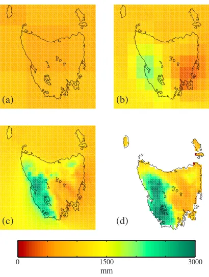
0 1500 3000

mm

(a) (b)

(c) (d)

elements from land and atmosphere. As such, in our downscal-ing, CCAM introduces new structural error factors and its own internal variability responses, forced in a one-way direction from the bias adjusted SSTs. Therefore, this provides a down-scaling of the host GCM’s SSTs/ice to the exclusion of the global modes of atmospheric variability of the host GCM.

[19] For the second stage, CCAM was configured with

48 × 48 cells on each face (termed C48 hereafter) to produce thefine-scale simulations. Computational limits and the use of hydrostatic equations determined a final resolution of approximately 0.1° (~10 km) over a primary face covering Tasmania and its offshore islands. Thefine-resolution C48 simulations used the same bias-adjusted SST from the host GCM as bottom boundary conditions. To ensure that realisti-cally resolved systems will be advected into thefine-resolution region of the C48 grid, we implemented a scale-selectivefilter [Thatcher and McGregor, 2009] to nudge the atmosphere of the C48 model with the output from the C64 model. The spec-tral nudging is performed on the surface pressure, windfields, temperature, and atmospheric moisture above 850 hPa. The length scale of the spectral nudging is approximately the side length of the primary face. Thatcher and McGregor[2009] have shown that nudging these variables results in a consistent improvement in pattern correlation and root-mean-square errors at the surface and the 500 hPa level. Again, the atmo-spheric composition and radiative forcing were the same as the host GCM and the simulations were run with a 6 min time step with output from most variables saved every 6 h.

[20] Finally, the model output from the CCAM conformal

grid is regridded to a geodetic system grid (WGS84) with a horizontal resolution of 0.1° (~10 km) over Tasmania and output time step of 6 h.

4. Evaluation

4.1. Simulations of Historical Climate

[21] The ability of the CCAM simulations to reproduce the

current observed temperature and rainfall climate is assessed as a means of estimating the reliability of projections of the future Tasmanian climate [Charles et al., 1999;Christensen and Christensen, 2007]. Simulated screen temperature and rainfall are compared to the Australian Water Availability Project (AWAP) [Jones et al., 2009] gridded climate data set. It should be noted that due to sparse station coverage and a high degree of spatial variation in climate across Tasmania, the AWAP-observed gridded data set may not ac-curately represent historical climate, especially for the sparsely monitored west and southwest of Tasmania [Beesley et al., 2009;Jones et al., 2009]. The spatial and temporal variabil-ities of mean rainfall and temperature are compared in this section. Further evaluation is presented in Bennett et al. [2010, 2012] using this model output in hydrological models in order to inform future water use in Tasmania.White et al. [2010, 2013] analyze the simulation of extreme temperature and precipitation whileHolz et al. [2010] analyze projected changes to agricultural indices and related variables. Grose et al. [2010, 2012, 2013] assess the ability of the simulations to replicate some relevant regional climate dynamics.

[22] Tasmania is approximately 350 km by 300 km and is

represented by 0 to 6 land cells in the 23 GCMs that partici-pated in CMIP3 [Meehl et al., 2007a]. At this resolution, GCMs are able to provide only very limited spatial differen-tiation across the state. With the increased resolution through the downscaling process, the regional differences in mean annual temperature and rainfall that exist in Tasmanian climate are simulated with greaterfidelity. Examining GFDL-CM2.1 as an example (other simulations show a very similar pat-tern), the mean annual rainfall and temperature in the GCM and the 0.5° CCAM simulations are spatially coarse and obviously do not resolve the regional detail present in the 0.1° model output or the gridded observations (Figures 3 and 4). These improvements can be quantified by comparing with the AWAP gridded observations. When comparing the 0.1° simulation to AWAP gridded data (upscaled to 0.1° from a native resolution of 0.05° so as to be directly compa-rable), the spatial correlation for mean monthly temperature is 0.93, while for rainfall, it is 0.86. In comparison, the GCM has a spatial correlation of 0.45 for temperature and 0.28 for rainfall compared to observations. The intermedi-ate-resolution 0.5° model lies between the two with spatial

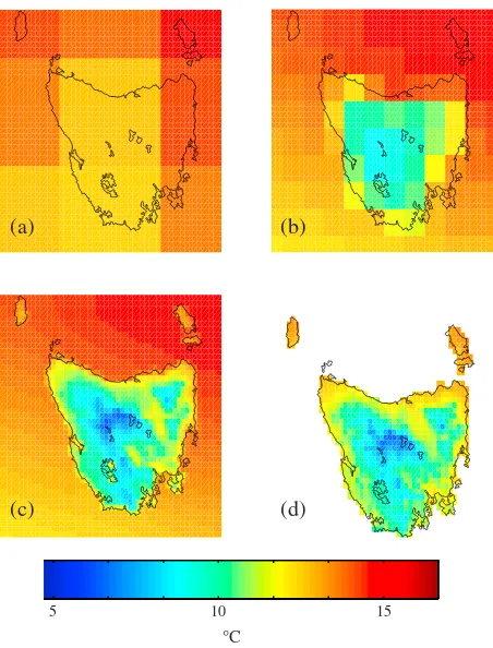
5

°C

(a) (b)

(c) (d)

10 15

Figure 4. Mean temperature (°C) over Tasmania for the period 1961–1990 from (a) the GCM GFDL-CM2.1, (b) the 0.5° downscaled simulation of the same GCM, (c) the 0.1° downscaled simulation of the same GCM, and (d) the gridded AWAP observations interpolated to 0.1°.

Table 1. Spatial Correlations for Rainfall and Temperaturea

Model Resolution Mean Monthly Temperature Mean Monthly Rainfall

GCM 0.45 0.28

0.5° 0.79 0.44

0.1° 0.93 0.86

a

correlations of 0.79 and 0.44, respectively (see also Table 1 for correlations as function of scale and variable).

[23] Higher resolution should improve the simulations of

spatial patterns of rainfall. Due to the inclusion of topogra-phy, the downscaled simulations exhibit more realistic orographic effects on rainfall than GCMs and thus would be expected to produce more rain. This is indeed the case: The mean annual rainfall of the entire region, shown in Figure 3 (Tasmania and the immediately surrounding ocean), is 750 mm for the GCM, while for the 0.5° and 0.1° simula-tions, it is 1010 mm and 1175 mm, respectively. If we just consider the land area, then the mean annual rainfall from the 0.1° simulations is 1385 mm. This is very close to the AWAP mean rainfall of 1390 mm. For temperature, the pres-ence of topography is expected to lead to a slight reduction in mean annual temperature due to the cooler temperatures that exist at altitude, and this can be seen in Figure 4. The mean annual temperature for the Tasmanian region from the GCMs is 14.1°C, for the 0.5° simulation it is 13.7°C and for the 0.1° simulation it is 13.5°C.

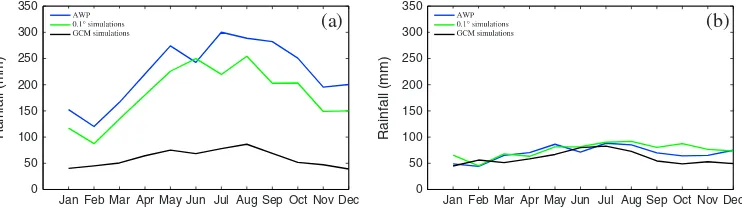
[24] Similar improvements through increased resolution can

be seen in the modeling of seasonal variation of rainfall over Tasmania (Figure 5 and Table 2). The west coast region of Tasmania has a strong seasonal rainfall cycle in the AWAP observations, with more rain falling in winter than in summer. In contrast, east coast rainfall is not strongly seasonal. Due at least in part to the lack of topography (and in some cases, land grid cells), the GCMs cannot reproduce this difference be-tween west and east coast rainfall. In contrast, the downscaled 0.1° simulations faithfully reproduce a strong seasonal cycle for the west coast and the absence of a seasonal cycle in monthly rainfall for the east coast. In other regions of the state (the north, the midlands, and the southeast), the downscaled simulations show a similar ability to reproduce the observed seasonal cycle (not shown). The realistic simulation of sea-sonal rainfall patterns for the east and west of Tasmania agrees withGrose et al. [2012, 2013] whofind that CCAM is better able to discern the differing weather systems that affect the east and west coasts than GCMs.

[25] A number of authors have recently sought to establish

the extent to which regional climate models“add value”to global climate models, assessed through their ability to simu-late the current climate [e.g., Feser et al., 2011;Kanamitsu and DeHaan, 2011]. Addressing this question is difficult, in part because global climate models are designed to simulate global- and continental-scale climates and cannot hope to rep-licate subgrid-scale features (as demonstrated above), while

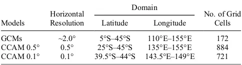
regional models are not usually assessed over global domains. UsingTaylor[2001] diagrams, we assess the capacity of the simulations to simulate the spatial distributions present in AWAP over a spatial domain relevant to the resolution of the simulation. Simulated rainfall in the historical climate (1961–1990) has been compared to gridded AWAP obser-vations (Figure 6) for the host GCMs as well as the two downscaled resolutions (0.5° and 0.1°). We tested each set of simulations at their native resolution over a domain that suited its purpose (from continental scale for the GCM to Tasmania-wide for the 0.1° simulations). Using different domains to compare model performance has the obvious detraction that we are not comparing performance over the same climatic zones; however, this analysis shows how well models at each resolution perform the task for which they are designed and indicates the level of value that downscaling adds to the GCM simulations. A similar, or even improved, skill score in the downscaling at a smaller domain indicates that the model is performing comparably to the host GCM but at a more regional scale, and thus the downscaling process is successful at allowing us to model the climate on a smaller scale. Only land cells are assessed. GCMs are regridded to match the highest-resolution GCM (CSIRO-Mk3.5, an approximate horizontal resolution of 2°). For GCMs, we have assessed only regions where all six GCMs have land cells (Figure 6, left column). We use a continent-scale domain to assess GCMs (Figure 6 and Table 3), following other studies [e.g.,Smith and Chandler, 2010]. The 0.5° simulations are assessed over southeast Australia, while the 0.1° simulations are assessed over Tasmania (Figure 6 and Table 3). AWAP rainfalls are regridded on to the 2° and 0.5° grids in order to match the resolution of the simulations.

[26] Spatial correlations improve from 0.6 to 0.8 in the

GCM simulations to about 0.9 in the 0.5° and 0.1° down-scaled simulations, while spatial variance more closely

Jan Feb Mar Apr May Jun Jul Aug Sep Oct Nov Dec Jan Feb Mar Apr May Jun Jul Aug Sep Oct Nov Dec 0

50 100 150 200 250 300 350

Rainfall (mm)

AWAP 0.1o simulation

GCM simulations (a)

0 50 100 150 200 250 300 350

Rainfall (mm)

AWAP 0.1o simulation

GCM simulations (b)

Figure 5. The monthly cycle of rainfall for the period 1961–1990 for observations, GCM six-model mean, and 0.1° downscaled simulations six-model mean for (a) the west coast and (b) the east coast regions of Tasmania.

Table 2. Mean and Variance of Monthly Rainfalla

Mean Monthly Rainfall (mm)

West Coast East Coast

Mean Variance Mean Variance

AWAP 224 55 70 14

GCM 60 16 60 13

0.1° 181 54 75 14

a

matches AWAP observations in the downscaled simulations (Figure 6, right column). These represent marked increases in skill over the raw GCM simulations, as observed mean annual rainfalls show considerably greater spatial variation and span markedly larger ranges of values in the 0.5° and 0.1° modeling output. The root-mean-square differences (RMSDs) decrease from the GCM to the 0.5° simulations but increase slightly again in the 0.1° simulations. The increas-ing RMSD in the 0.1° simulations reflects the increasing complexity of the spatial pattern of Tasmanian rainfall (and the higher overall rainfall) in relation to rainfall of southeastern Australia. Also, the higher RMSD is to be expected, due to the higher signal-to-noise ratio of the climate atfiner spatial scales. The spatial standard deviation in the 0.1° simulations is much closer to the variability of AWAP than is the case for the 0.5° or GCM simulations. Overall, the fact that the spa-tial biases are similar or even improved as we downscale from GCMs tofiner resolution indicates that the CCAM simulations are performing with comparable, or improved,fidelity for their target resolution compared to the host GCM.

[27] There is a notable reduction in model spread in both

spatial correlation and standard deviation in CCAM com-pared to the GCM simulations. For example, considerable differences in spatial deviation exist between the GCMs, yet the 0.5° simulations forced by those GCMs are largely indistinguishable from each other (Figure 6). The reduction of spread in the ensemble is caused by a combination of the bias correction of SSTs before downscaling and the use of a single downscaling model. CCAM generates its own atmo-sphere and therefore applies a consistent set of parameters and physical equations to GCM SSTs, thereby reducing the variation between simulations. Other downscaling methods may show a different spread of RMSD and correlation

coef-ficients given the same GCM inputs [Murphy, 2000]. This SST bias adjustment is a likely cause for the clustering of

simulations, especially in regard to RMSD; however, the magnitude of this clustering cannot be quantified without more controlled tests.

4.2. Applicability of Output for Impacts Research

[28] The realistic simulation of the spatial and temporal

patterns of rain is important for the downscaled simulations to be used directly in impacts research including applied models. Figure 7 shows the spatial distribution of the number of days with certain volumes of rain in both observed data (top row) and six-model-mean (bottom row). Regular rain-falls, including heavy rainrain-falls, occur on the west coast as a result of the interaction between regular westerly weather systems, such as fronts and troughs, with western and central mountains [Langford, 1965]. A strong east-west gradient in all rainfall categories is clearly evident in observations; there are far fewer days on the west coast compared to the east coast with no or light rain (<5 mm/d) and the opposite is true for heavy rain (>30 mm/d). The modeled rainfall distri-butions show the same east-west distribution as the obser-vations; the spatial correlation between the observed and modeled rainfall days is above 80% for three of the four plots (82% for days with no rain, 88% for days with<5 mm rain, and 86% for days with>15 mm rain). For days with greater than 30 mm of rain, the correlation is still high at 62%. As

Figure 6. Performance of rainfall simulations at different resolutions and over different domains. (top row) Mean annual rainfall for 1961–1990 from the AWAP data set for grid cells and domains used to assess the (left column) GCM simulations (~2.0°), the (middle column) 0.5° RCM simulations, and the (right column) 0.1° RCM simulations. (bottom row)Taylor(2001) diagrams comparing spatial characteristics of simulated rainfalls with corresponding AWAP rainfalls shown in (top row). Magenta diamonds show AWAP rainfalls. Each RCM simulation is named from the forcing GCM. Blue hexagrams show control RCM simulations forced by NCEP reanalysis.

Table 3. Domains Over Which Rainfall Simulation Performance Is Assessed

Models

Horizontal Resolution

Domain

No. of Grid Cells Latitude Longitude

GCMs have no more than two cells to span Tasmania and very little or no topographic difference in these cells, it is not possible to differentiate between the character of east and west Tasmanian rainfall. This output was used success-fully in biophysical [Holz et al., 2010] and hydrological models [Bennett et al., 2012], indicating that the biases were acceptable for these purposes.

[29] Further evaluation of the variability in the simulations

for use in applied models is examined through frequency dis-tributions at point locations. Frequency disdis-tributions of a number of rainfall characteristics are also improved. The downscaling process employed provides improvements to the simulated frequency distributions of daily rainfall for the downscaled model relative to the host GCM. This

Figure 7. Comparison of the distribution of daily rainfall in (a–d) AWAP and (e, f) the six-model mean for the months May–August for the period 1961–1990. Displayed is the number of days per year with no rain, less than 5 mm of rain, greater than 15 mm of rain, and greater than 30 mm of rain.

0.1o Model Mean AWAP GCM Model Mean

Melaleuca - daily rainfall

Daily Rainfall (mm)

Log

10

(No. of days/year)

2.5

2

1.5

1

0.5

0

Log

10

(No. of days/year)

2.5

2

1.5

1

0.5

0 (c)

0.1o Model Mean AWAP GCM Model Mean

Miena - daily rainfall

Daily Rainfall (mm)

(d)

0.1o Model Mean AWAP GCM Model Mean

Melaleuca - daily max temperature

Te mperature (°C)

No. of days/year

60

40

20

0 0

0 5 10 15 20 25 30 0 5 10 15 20 25 30

10 20 30 40 0 10 20 30 40

(a)

0.1o Model Mean AWAP GCM Model Mean

Miena - daily max temperature

Te mperature (°C)

No. of days/year

60

40

20

0 (b)

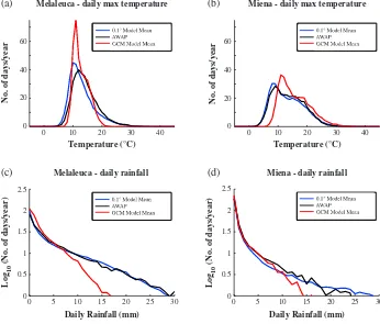
improvement is highlighted for two distinct locations: Melaleuca in Tasmania’s far southwest and Miena in the cen-ter of the state (Figure 8). This analysis has been carried out using CSIRO-Mk3.5 as host GCM (other models showed a very similar result, not shown). The observations are repre-sented by the AWAP gridded observations corresponding to that point rather than station data as the comparison between gridded observations and gridded model output allows for a more accurate assessment of the performance of the model than does a comparison with station records.

[30] Previous studies for the Australian region have found

that GCMs have some skill at simulating the observed tem-poral variability of temperature and precipitation extremes when averaged over the whole of the Australian continent [Alexander and Arblaster, 2009]. In this study however, the coarse-resolution GCM simulations were largely found to be unable to reproduce the variability of the AWAP obser-vations for the Tasmania region with any significant skill, particularly at the more extreme ends of the temperature and precipitation distributions [White et al., 2013]. In the southwest of the state for example (Melaleuca, Figure 8), the GCM overestimates the number of days at or near aver-age temperature while underestimating the hot and cold extremes at both ends of the frequency distribution. In the central highlands (Miena), the GCM significantly under-estimates the cold end of the distribution but overunder-estimates high temperatures. By contrast, the downscaling process was found to significantly improve the frequency distribu-tions of temperature when compared to the host GCM.

[31] We use the probability density function (PDF) skill

score,Sscore, ofPerkins et al. [2007] to assess the similarities between simulated and observed PDFs.Sscoreis calculated by

Sscore¼

Xn

1

minimumðZm; ;ZoÞ; (2)

where n is the number of bins into which the PDFs are divided,Zmis the value of the modeled probability density

for bin n, and Zo is the value of the observed probability density for bin n. A PDF skill score of 1 indicates perfect agreement between PDFs, while a score of 0 means no overlap (seePerkins et al. [2007] for further discussion of this score). The PDF skill score for the mean daily maximum temperature and daily precipitation over the period 1961–1990 for both the GCM and 0.1° downscaled simulations relative to AWAP shows the improvement through downscaling (Table 4). At both locations, the skill score for temperature showed a sig-nificant improvement. This can also be seen in Figure 8, where the frequency distribution for the GCMs overestimates the number of middle-temperature days and underestimates extremes at both ends.

[32] Comparison between the PDF skill scores for the GCM

and the 0.1° downscaled simulations for rainfall shows a sim-ilar improvement (Table 4). For the GCM, events greater than 17 mm of rain per day have a frequency of near zero at both locations, which shows a serious underestimation of extreme rainfall. By contrast, the frequency distributions of 0.1° down-scaled simulation closely follow the AWAP-observed distri-butions at both locations, although at Miena, the downscaled simulations show a tendency to overestimate heavy rainfall compared to the AWAP observations. This is reflected in the PDF skill score, which shows only a much smaller improve-ment. PDF skill scores for the 0.5° simulations (not shown) were between those obtained for the GCM and those for the 0.1° simulations. These results are in agreement withWhite et al. [2010, 2013] who found good agreement between AWAP observations and the range of the six 0.1° down-scaled simulations using a suite of extreme temperature and rainfall indices across Tasmania. The ability of the down-scaled simulations in modeling different PDFs for locations that occur within the same GCM grid cell was crucial for successfully capturing realistic rainfall and thus runoff and river flows through hydrological modeling [Bennett et al., 2012].

[33] We note, however, that CCAM has a tendency to not

simulate rainfall autocorrelation characteristics realistically. CCAM underestimates the length of both dry spells [White et al., 2013] and the duration (and accumulated rainfall) of multiday rainfall events [Bennett et al., 2013]. These biases reduce the confidence in the projection of rainfall variability by CCAM, since they may indicate deficiencies in the simu-lation of the processes that bring rainfall and where the mean rainfall matches observations, this may indicate compensat-ing effects between multiple errors. This can be examined through process studies of the model dynamics. For example,

Grose et al. [2012] showed that CCAM displays biases in the

Table 4. PDF Skill Score for GCM and Downscaled Modela

Miena Melaleuca

Temperature Rainfall Temperature Rainfall

GCM 0.7983 0.9020 0.7945 0.8004

0.1° model 0.9542 0.9419 0.8650 0.9411

a_{PDF skill score against AWAP for GCM (CSIRO-Mk3.5) and}

down-scaled 0.1° CCAM for daily maximum temperature and daily precipitation at Miena and Melaleuca for the period 1961–1990.

Change GCM Precipitation (mm)

140 150 160

Change 0.5° Precipitation (mm)

20

0 %

-20

Change 0.1° Precipitation (mm)

-35

-40

-45

Longitude °

-35

-40

-45

-40

-42

-44

Longitude ° Longitude °

Latitude°

140 150 160 144 146 148

Latitude° Latitude°

(a) (b) (c)

mean circulation, atmospheric blocking, and the frequency, extent, and mean latitude of cutoff lows, an important mech-anism for large rainfalls over east Tasmania. However,Grose et al. [2012] also demonstrated that CCAM represents all these features more realistically than an example GCM (CSIRO-Mk3.5), indicating that even here CCAM adds value to GCM simulations. There may be biases in other im-portant synoptic features, such as the fronts and troughs em-bedded in the westerlyflow that bring the dominant rainfall to the west coast.

4.3. Future Projections

[34] The purpose of downscaling GCMs is to increase our

understanding of the regional changes that are projected for the future. The purpose is not to create detailed-looking data sets since these can be created using other means. Therefore, it is useful to examine the projected change in the downscal-ing in comparison to the host GCMs. Further information in the projected climate-change signal, including more regional detail, is the basis for a common definition of“added value” in downscaling [e.g., Di Luca et al., 2012]. Downscaled models are most valuable when they can offer insight into processes that are beyond the resolution of GCMs.

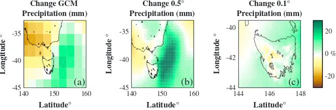
Here we compare the rainfall change between 1961–1990 and 2071–2100 under the A2 scenario and demonstrate how downscaling allows for a different rainfall response over a region than is projected using GCMs alone. Figure 9 shows the projected rainfall change from GCMs, the 0.5° simula-tions and the 0.1° simulasimula-tions. The GCMs project, on aver-age, a decrease in rainfall in the central and western north of the state, no change in the southwest, and an increase in rain in a strip along the northeast coast. The 0.5° simulations extend the region of increased rain farther west and into the southwest of the state. Significantly, these simulations also project a much greater increase in rain just off the east coast of Tasmania (in excess of 20%) and an increase in rain along the east coast of mainland Australia and into the Alps region (where the GCMs project a decrease). The region of rainfall increase to the east and northeast of Tasmania coincides with a region of larger SST increase associated with a southward extension of the East Australia Current. The 0.1° simulations project an increase in rain along almost the entire coastline (except for the central west), with the only area of drying being the Central Plateau and west coast. Crucially, the region of increased rain is extended from just a strip along the east coast to the entire north east of the state, as well as the south-east and north coast. This response is present in the six-model mean and is also consistent across the six simulations.

[35] This level of regional response is important, for example,

in light of the proposed irrigation developments in Tasmania’s northeast. The added detail in the downscaling means that for some individual locations the model mean projection shows the opposite sign compared to the host models (e.g., the north-east). The difference in response in CCAM compared to the GCMs is even more marked in individual seasons, with some marked regional patterns emerging in austral summer and austral winter. These differences between GCM and RCM output will have important implications for climate change impact and adaptation work. Where the trend is different, those undertaking adaptation or impact work will need to either increase the envelope of uncertainty to include both results or decide which scale of modeling is more likely. It is important that those undertaking downscaling of GCMs pro-vide justification for results that are different to those given by GCMs. The difference in projected seasonal rainfall change between the east and west halves of Tasmania is consistent with a different relationship to mean westerly circulation and other rainfall drivers. For a more detailed explanation of the likely physical validity of these results, and how theyfit in with larger-scale trends, seeGrose et al. [2013].

[36] As well as examining the regional patterns of projected

changes, we examine the projected mean change of tempera-ture and rainfall in Tasmania as a whole. This places the range of projections from the downscaling in the broad context of change for the region. A simple delta scaling process would yield near-identical projected changes as GCMs for the region as a whole. Using a statistical downscaling, it is possible to get results that are in opposition to the GCM for small regions; however, most forms of statistical downscaling assume that the relationships between large-scale trends from the GCM and local conditions are maintained [Cubasch et al., 1996;

Murphy, 2000], and thus in most cases, the trend in the stat-istically downscaled model is consistent with the GCM. The dynamical downscaling method employed, including aspects such as SST bias correction, running an entirely new

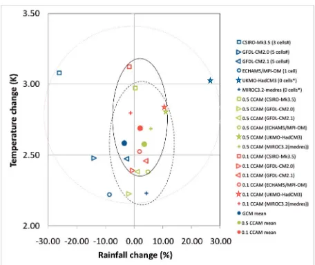
atmospheric model, and increased resolution of surface forc-ings like topography and coasts, has resulted in the projected trends in CCAM being different from the host GCMs used as input. If the range between different GCMs is taken as a plausible range of future conditions, a reduction in this range through downscaling may be interpreted as a fault since it pro-duces a skewing of the distribution of projections. Alternatively, the presence of consistent regional patterns in the downscaling, such as the increase in rainfall on the east coast that was not present in the host GCMs, might produce a different range of projected change at the statewide scale that can be viewed with greater confidence than the host GCMs. The statewide projected change is shown by the phase space of projected change in Tasmanian mean temperature and rain-fall over the 21st century under the A2 scenario shown in Figure 10, similar to the approach ofWhetton et al. [2012]. The most notable features are the reduced model range of projected change through each stage of downscaling, espe-cially for the rainfall indices, and a shift in the multimodel mean value of change.

[37] The model spread of future projected mean

tempera-ture change is less in the CCAM simulations than for the GCMs. The multimodel mean value of projected temperature change is the same in the GCMs and the 0.5° simulations but is 0.11 °C higher in the 0.1° simulations. For mean rainfall, the model spread is much greater in the GCM simulations (26% to 27%) than in the 0.5° CCAM simulations (2% to 11%). The model spread in the 0.1° CCAM simulations is similar to the 0.5° simulations (2% to 10%). The multimodel mean projected rainfall change is slightly negative in the GCMs and slightly positive in the CCAM simulations; how-ever, all values are<4%. The reduction in model spread and a change in the multimodel mean values of change reflect a number of influences. It shows the effect of using a single atmospheric model (CCAM) in these simulations and a single model configuration for the region (e.g., atmospheric processes, coastline, topography, etc.). In addition, SST bias adjustment of the GCM input causes a reduction in model spread, as explained above, for the current climate. The resulting reduction of atmospheric biases in the current climate, such as the mean latitude of westerly storm tracks in CCAM [Grose et al., 2013], may have contributed to the reduction of outliers in the projection of rainfall. Also, as mentioned above, the inclusion of processes atfiner length scales in the downscaling model, such as the effect of topog-raphy, is expected to influence not only the simulation of the current climate but also the projected climate change signal at the statewide scale. This last influence is especially important to explain the differences between the 0.5° and 0.1° CCAM simulations, where the model is the same. The regional fea-tures that were consistently introduced by the downscaling and appear physically plausible, such as the different sign of projected rainfall change in the western district and the northeast of Tasmania, are expected to be an important con-tribution to the difference in the spread of projected change for Tasmania between the downscaling and GCMs.

5. Discussion and Conclusions

[38] The uncertainties in our knowledge of the Earth system

in climate projections (that is, the uncertainty in the range of responses in the climate system given a prescribed

emissions scenario) can be partially quantified by analyzing the range of projections of multimodel ensembles [Palmer et al., 2005]. For a given emissions scenario, GCM ensembles may be employed to reflect uncertainties in our understanding of physical climate processes as well as limitations in com-puter simulations of known climate processes [Meehl et al., 2007b]. However, the magnitude of some climate-change signals reported by GCMs has been shown to be correlated with model biases; for example, the poleward movement of the Southern Hemisphere storm tracks in response to green-house forcing is correlated with the present bias in their latitude [Kidston and Gerber, 2010]. This implies that GCMs may respond differently to anthropogenic global warming scenar-ios due to biases rather than to uncertainties in our understand-ing of physical climate processes or computational limitations. [39] By bias adjusting GCM SSTs before downscaling, we

have attempted to reduce uncertainty in climate change pro-jections caused by model-specific GCM biases. Each method of downscaling inherits biases from the host model and also introduces some biases and uncertainty specific to the model [Foley, 2010]. This downscaling method does inevitably introduce its own uncertainties and biases but achieves a reduction in biases in inputs from the host model. Ourfindings support those of Nguyen et al. [2011], who find that bias adjusting GCM SSTs before downscaling contributes to improved simulation of current climate. This technique is only possible through the use of a stretched-grid global atmospheric model as these models are able to operate without the use of horizontal atmospheric boundary conditions. The downscal-ing method we have employed therefore has the dual benefits of creating afiner resolution product (both temporally and spa-tially) and reducing the bias of the model output compared to the current climate, relative to global climate model output. Finally, much of the spread across the ensembles of CMIP3 models occurs through model differences in the mean state of the climate [Randall et al., 2007], and not from temporal variability. Consequently, the removal of biases through bias adjustment means that the underlying mean state coincides with the observed climate and thus the intermodel uncertainty in the projections is narrowed.

[40] The bias adjustment of SST in a host GCM prior

to downscaling has been explored in a number of recent papers [Nguyen et al., 2011;Maraun, 2012;White and Toumi, 2013]. The stationarity of the SST bias is a crucial assumption for this process [Ashfaq et al., 2011;Maraun, 2012], but one that is difficult to validate. The split-sample cross-validation tech-nique employed in this paper demonstrates that the bias adjust-ment was relatively insensitive to the size of the training period. A similar experiment was undertaken using 15 year periods from the beginning (1950–1964) and end (1985–1999) of the observational window (results not shown) and this did not indicate any trend in bias over this period.

[41] Some form of downscaling is essential in order to

dynamical downscaling [Cubasch et al., 1996;Murphy, 1999;

Fowler et al., 2007;Fowler and Wilby, 2007]. In general, the two downscaling methods perform similarly for present-day climate; however, the two methods often differ when applied to future climate projections [Cubasch et al., 1996;Murphy, 2000]. The best method of downscaling often depends on a combination of the application of the model output along with the season and location under study [Diez et al., 2005] as well as available expertise.

[42] Simple forms of scaling observations using the climate

change signal from GCM outputs can produce usable outputs but offer limited“added value”in the projected climate change signal relative to GCMs. Most forms of statistical downscaling are limited by the assumption that observed links between large-scale climate variables (from the GCM) and local cli-mate will persist in a changed clicli-mate regime. Also, it is diffi -cult to resolve changes to timing and frequency (seasonality) of weather events using statistical downscaling [Cubasch et al., 1996]. Weather generators overcome these problems but the stochastic nature of these generators and the difficulty with implementing multivariate extreme value statistics intro-duce problems of their own [Maraun et al., 2010]. Dynamical downscaling offers the possibility of added value and regional detail in the climate change signal, as well as a fully modeled response in variability and extremes that includes events that are outside the current observed range. However, the dy-namical model outputs must be carefully validated against ob-servations to assess their usefulness and biases.

[43] The use of dynamical downscaling in this study allows

us to demonstrate changes in the local climate of Tasmania, such as changes to seasonality, frequency, and timing of weather events. The downscaled simulations also better reflect the complex relationships between interacting climate drivers across Tasmania, such as the different relationship between mean rainfall and mean westerly circulation in the west com-pared to the east [Grose et al., 2012]. Furthermore, using only bottom boundary conditions in the form of bias-adjusted SSTs to force the downscaled model allows us to simulate regional-scale changes that are in contrast to the trend generated by the host GCM (e.g., Figure 9), while illustrating a plausible pattern of regional projected change at the scale of Tasmania that could not be achieved using simple scaling of GCM outputs.

Grose et al. [2012, 2013] demonstrate that the changes suggested by the 0.1° simulations are both physically consis-tent with changes in mean circulation and specific synoptic drivers and provide plausible changes based upon the large-scale changes projected for the climate in the Australian region. [44] The timing and intensity of rainfall events can be as

important as the annual or seasonal mean total rainfall in determining water availability [Bennett et al., 2010; Bennett et al., 2012]. We have shown that our dynamical downscaling method can reproduce the observed spatial distribution of rain-fall events across a range of intensities (Figure 7) as well as the probability distribution functions of rain (Figure 8). A decent validation of variability in the current climate gives confidence that the model projection of variability by the downscaling model is plausible. Being able to reproduce observations with highfidelity is useful as it allows model output to be used in application models such as hydrological or biophysical models, with only minor bias adjustment of the output. This allows the full climate change signal projected by the model, including changes to mean and variability and extremes, to be accounted

for in impacts research. Many of these impact models, such as DairyMod [Johnson et al., 2008] or ApSim [Keating et al., 2003], are tuned to observed conditions and have strong nonlinear responses to temperature and rainfall; thus, a small bias in the model output can generate wildly inaccurate responses. Thefine-scale model output from this project has been successfully used in a number of studies with only min-imal bias adjustment of the model output [Corney et al., 2010;

Bennett et al., 2012;Bennett et al., 2013]. These studies in-clude a number of agricultural applications [Holz et al., 2010], hydrology [Bennett et al., 2010, 2012], extreme events [White et al., 2010;White et al., 2013], changes to the environ-ment of Tasmania’s freshwater fish [Morrongiello et al., 2011], and an assessment of changes to wind risk across Tasmania [Cechet et al., 2012].

[45] The downscaling method increases the regional climate

information content over a wide range of temporal scales, whilst reducing biases in the present-day climatology. This then allows detailed use of highly nonlinear discipline-specific models to understand the important impacts and consequences of rising greenhouse concentrations.

[46] Acknowledgments. This work was part of the Climate Futures for Tasmania project (CFT) (http://www.acecrc.org.au/Research/Climate% 20Futures). CFT was made possible through funding and research support from a consortium of state and national partners. The work was supported by the Australian government’s Cooperative Research Centres Program through the ACE CRC. We acknowledge the modeling groups, the Program for Climate Model Diagnosis and Intercomparison (PCMDI) and the WCRP’s Working Group on Coupled Modeling (WGCM), for their roles in making available the WCRP CMIP3 multimodel data set. Support for this data set is provided by the Office of Science, U.S. Department of Energy. The contribution of ARC Centre of Excellence for Climate Systems Science is acknowledged by NLB (CE11E0098). We thank W. F. Budd (ACE CRC) for comments and discussion. Finally, we acknowledge the three anonymous reviewers whose comments have improved this paper.

References

Alexander, L. V., and J. M. Arblaster (2009), Assessing trends in observed and modelled climate extremes over Australia in relation to future projec-tions,Int. J. Climatol.,29, 417–435.

Ashfaq, M., C. B. Skinner, and N. S. Diffenbaugh (2011), Influence of SST biases on future climate change projections,Clim. Dyn.,36, 1303–1319. Beesley, C., A. Frost, and J. Zajaczkowski (2009), A comparison of the

BAWAP and SILO spatially interpolated daily rainfall datasets. Pages 3886–3892 in World IMACS/MODSIM Congress, Cairns.

Bennett, J. C., F. L. N. Ling, B. Graham, S. P. Corney, G. K. Holz, M. R. Grose, C. J. White, S. M. Gaynor, and N. L. Bindoff (2010),Climate Futures for Tasmania: Water and Catchments Technical Report, Antarctic Climate and Ecosystems Cooperative Research Centre, Hobart, Tasmania. Bennett, J. C., F. L. N. Ling, D. A. Post, M. R. Grose, S. P. Corney, B. Graham,

G. K. Holz, J. J. Katzfey, and N. L. Bindoff (2012), High-resolution projec-tions of surface water availability for Tasmania, Australia,Hydrol. Earth Syst. Sci.,16, 1287–1303.

Bennett, J. C., M. R. Grose, S. P. Corney, C. J. White, G. K. Holz, J. J. Katzfey, D. A. Post, and N. L. Bindoff (2013), Performance of an em-pirical bias-correction of a high-resolution climate dataset, Int. J. Climatol., doi:10.1002/joc.3830.

Berbery, E. H., and M. S. Fox-Rabinovitz (2003), Multiscale diagnosis of the North American Monsoon System using a variable-resolution GCM, J. Clim.,16, 1929–1947.

Boberg, F., and J. H. Christensen (2012), Overestimation of Mediterranean summer temperature projections due to model deficiencies, Nat. Clim. Change,2, 433–436.

Boe, J., L. Terray, F. Habets, and E. Martin (2007), Statistical and dynamical downscaling of the Seine basin climate for hydro-meteorological studies, Int. J. Climatol.,27, 1643–1655.

Bureau of Meteorology (2008),Climate of Australia, Bureau of Meteorology, Melbourne.

Cechet, R. P., et al. (2012),Climate Futures for Tasmania: Severe Wind Hazard and Risk Technical Report, Geosciences Australia, Canberra, Australia. Charles, S. P., B. C. Bates, P. H. Whetton, and J. P. Hughes (1999), Validation

of downscaling models for changed climate conditions: Case study of south-western Australia,Clim. Res.,12, 1–14.

Chiew, F. H. S., J. Teng, J. Vaze, D. A. Post, J. M. Perraud, D. G. C. Kirono, and N. R. Viney (2009), Estimating climate change impact on runoff across southeast Australia: Method, results and implications of the modeling method, inWater Resour. Res.,45, W10414, doi:10.1029/2008WR007338. Christensen, J. H., and O. B. Christensen (2007), A summary of the PRUDENCE model projections of changes in European climate by the end of this century,Clim. Change,81, 7–30.

Christensen, J. H., et al. (2007), Regional climate projections, in The Physical Science Basis. Contribution of Working Group I to the Fourth Assessment Report of the Intergovernmental Panel on Climate Change, edited by S. Solomon et al., pp. 847–940, Cambridge Univ. Press, Cambridge, United Kingdom and New York, N.Y., U.S.A.

Christensen, J. H., F. Boberg, O. B. Christensen, and P. Lucas-Picher (2008), On the need for bias correction of regional climate change projections of temperature and precipitation, Geophys. Res. Lett., 35, L20709, doi:10.1029/2008GL035694.

Corney, S. P., J. K. Katzfey, J. McGregor, M. Grose, C. White, G. Holz, J. Bennett, S. Gaynor, and N. L. Bindoff (2010),Climate Futures for Tasmania: Methods and Results on Climate Modelling, Antarctic Climate and Ecosystems Cooperative Research Centre, Hobart.

Cubasch, U., H. von Storch, J. Waszkewitz, and E. Zorita (1996), Estimates of climate change on southern Europe derived from dynamical climate model output,Clim. Res.,7, 129–149.

Di Luca, A., R. de Elia, and R. Laprise (2012), Potential for added value in precipitation simulated by high-resolution nested regional climate models and observations,Clim. Dyn.,38, 1229–1247.

Diez, E., A. Primo, J. A. Garcia-Moya, J. M. Guttierez, and B. Orfila (2005), Statistical and dynamical downscaling of precipitation over Spain from DEMETER seasonal forecasts,Tellus Ser. a Dyn. Meteorol. Oceanogr., 57, 409–423.

Engelbrecht, F. A., J. L. McGregor, and C. J. Engelbrecht (2009), Dynamics of the Conformal-Cubic Atmospheric Model projected climate-change signal over southern Africa,Int. J. Climatol.,29, 1013–1033.

Feng, J., D.-K. Lee, C. Fu, J. Tang, Y. Sato, H. Kato, J. L. McGregor, and K. Mabuchi (2011), Comparison of four ensemble methods combining regional climate simulations over Asia,Meteorol. Atmos. Phys.,111, 41–53. Feser, F., B. Rockel, H. von Storch, J. Winterfeldt, and M. Zahn (2011), Regional climate models add value to global model data: A review and selected examples,Bull. Am. Meteorol. Soc.,92, 1181–1192.

Foley, A. M. (2010), Uncertainty in regional climate modelling: A review, Prog. Phys. Geogr.,34, 647–670.

Fowler, H. J., and R. L. Wilby (2007), Beyond the downscaling comparison study,Int. J. Climatol.,27, 1543–1545.

Fowler, H. J., S. Blenkinsop, and C. Tebaldi (2007), Linking climate change modelling to impacts studies: Recent advances in downscaling techniques for hydrological modelling,Int. J. Climatol.,27, 1547–1578.

Fox-Rabinovitz, M., J. Côté, B. Dugas, M. Déqué, J. L. McGregor, and A. Belochitski (2008), Stretched-Grid Model Intercomparison Project: Decadal regional climate simulations with enhanced variable and uniform-resolution GCMs,Meteorol. Atmos. Phys.,100, 159–178.

Frost, A. J., et al. (2011), A comparison of multi-site daily rainfall downscaling techniques under Australian conditions,J. Hydrol.,408, 1–18.

Gates, W. L., et al. (1998), An overview of the results of the Atmospheric Model Intercomparison Project (AMIP I),Bull. Am. Meteorol. Soc.,73, 1962–1970.

Grose, M. R., I. Barnes-Keoghan, S. P. Corney, C. J. White, G. K. Holz, J. C. Bennett, S. M. Gaynor, and N. L. Bindoff (2010),Climate Futures for Tasmania: General Climate Technical Report, Antarctic Climate and Ecosystems Cooperative Research Centre, Hobart, Tasmania.

Grose, M., M. J. Pook, P. C. McIntosh, J. S. Risbey, and N. L. Bindoff (2012), The simulation of cutoff lows in a regional climate model: Reliability and future trends,Clim. Dyn.,39, 445–459.

Grose, M. R., S. P. Corney, J. K. Katzfey, J. C. Bennett, G. K. Holz, C. J. White, and N. L. Bindoff (2013), A regional response in mean west-erly circulation and rainfall to projected climate warming over Tasmania, Australia,Clim. Dyn.,40, 2035–2048.

Held, I. M., and B. J. Soden (2006), Robust responses of the hydrological cycle to global warming,J. Clim.,19, 5686–5699.

Holz, G., et al. (2010),Climate Futures for Tasmania: Impacts on Agriculture Technical Report, Antarctic Climate and Ecosystems Cooperative Research Centre, Hobart, Tasmania.

Hughes, L. (2003), Climate change and Australia: Trends, projections and impacts,Aust. Ecol.,28, 423–443.

Ines, A. V. M., and J. W. Hansen (2006), Bias correction of daily GCM rainfall for crop simulation studies,Agric. For. Meteorol.,138, 44–53.

IPCC (2007), Climate Change 2007: The Physical Science Basis. Contribution of Working Group I to the Fourth Assessment Report of the Intergovernmental Panel on Climate Change, Cambridge Univ. Press, Cambridge, U.K.

Johnson, I. R., D. F. Chapman, V. O. Snow, R. J. Eckard, A. J. Parsons, M. G. Lambert, and B. R. Cullen (2008), DairyMod and EcoMod: Biophysical pasture-simulation models for Australia and New Zealand, Aust. J. Exp. Agric.,48, 621–631.

Jones, D. A., W. Wang, and R. Fawcett (2009), High-quality spatial climate data-sets for Australia,Aust. Meteorol. Oceanogr. J.,58, 233–248. Kanamitsu, M., and L. DeHaan (2011), The Added Value Index: A new

metric to quantify the added value of regional models,J. Geophys. Res., 116, D11106, doi:10.1029/2011JD015597.

Katzfey, J. J., J. McGregor, K. C. Nguyen, and M. Thatcher (2009), Dynamical downscaling techniques: Impacts on regional climate change signals. 18th World IMACS Congress and MODSIM09 International Congress on Modelling and Simulation, edited by R. S. Anderssen, R. D. Braddock and L. T. H. Newham, Modelling and Simulation Society of Australia and New Zealand and International Association for Mathematics and Computers in Simulation: Cairns, pp. 3942–3947, Cairns. [Available online at http://www.mssanz.org.au/modsim09.]

Katzfey, J., J. L. McGregor, K. Nguyen, and M. Thatcher (2010), Regional climate change projection development and interpretation for Indonesia

final report for AusAID project. CSIRO Marine and Atmospheric Research, Melbourne.

Keating, B. A., et al. (2003), An overview of APSIM: A model designed for farming systems simulation,Eur. J. Agron.,18, 267–288.

Kidston, J., and E. P. Gerber (2010), Intermodel variability of the poleward shift of the austral jet stream in the CMIP3 integrations linked to biases in 20th century climatology,Geophys. Res. Lett.,37, L09708, doi:10.1029/ 2010GL042873.

Kowalczyk, E. A., J. R. Garratt, and P. B. Krummel (1994), Implementation of a soil-canopy scheme into the CSIRO GCM—Regional aspects of the model response. CSIRO Div. Atmospheric Research Tech. Paper. Lacis, A., and J. Hansen (1974), A parameterisation of the absorption of solar

radiation in the Earth’s atmosphere,J. Atmos. Sci.,31, 118–133. Lal, M., J. L. McGregor, and K. C. Nguyen (2008), Very high-resolution

climate simulation over Fiji using a global variable-resolution model, Clim. Dyn.,30, 293–305.

Langford, J. (1965),Weather and Climate, Lands and Survey Department, Hobart.

Lin, J. (2007), The double-ITCZ problem in IPCC AR4 coupled GCMs: Ocean-atmosphere feedback analysis,J. Clim.,20, 4497–4525. Maraun, D. (2012), Nonstationarities of regional climate model biases in

European seasonal mean temperature and precipitation sums,Geophys. Res. Lett.,39, L06706, doi:10.1029/2012GL051210.

Maraun, D., et al. (2010), Precipitation downscaling under climate change: recent developments to bridge the gap between dynamical models and the end user,Rev. Geophys.,48, RG3003, doi:10.1029/2009RG000314. McGregor, J. L. (2003), A new convection scheme using a simple closure.

Research Report 93, Bureau of Meteorology Research Centre, Melbourne. McGregor, J. L. (2005), CCAM: Geometric aspects and dynamical formulation.

Technical Paper 70, CSIRO Atmospheric Research, Melbourne. McGregor, J. L., and M. R. Dix (2001), The CSIRO Conformal-Cubic

Atmospheric GCM, inIUTAM Symposium on Advances in Mathematical Modelling of Atmosphere and Ocean Dynamics, edited by P. F. Hodnett, pp. 197–202, Springer, Netherlands.

McGregor, J. L., and M. R. Dix (2008), An updated description of the Conformal-Cubic Atmospheric Model, in High Resolution Numerical Modelling of the Atmosphere and Ocean, edited by K. Hamilton and W. Ohfuchi, pp. 51–75, Springer, New York.

McGregor, J. L., and K. Nguyen (2009), Dynamical downscaling from climate change experiments. Final report of Project 2.1.5b for the South Eastern Australian Climate Initiative. CSIRO Marine and Atmospheric Research, Melbourne.

McGregor, J. L., H. B. Gordon, I. G. Watterson, M. R. Dix, and L. D. Rotstayn (1993), The CSIRO 9-level atmospheric general circulation model. Technical Paper 26, CSIRO Atmospheric Research, Melbourne. Mearns, L. O., F. Giorgi, P. H. Whetton, D. Pabon, M. Hulme, and M. Lal

(2003), Guidelines for use of climate scenarios developed from regional climate model experiments. DDC of IPCC TGCIA.

Mechoso, C. R., et al. (1995), The seasonal cycle over the tropical Pacific in coupled ocean-atmosphere general circulation models, Mon. Weather Rev.,123, 2825–2838.

Meehl, G., A. C. Covey, T. Delworth, M. Latif, B. J. McAvaney, J. F. B. Mitchell, R. J. Stouffer, and K. E. Taylor (2007a), The WCRP CMIP3 multi-model dataset: A new era in climate change research,Bull. Am. Meteorol. Soc.,88, 1383–1394.